3.1. Physicochemical Parameters of Groundwater
The physicochemical characteristics of the groundwater resources in the CT aquifer contributed significantly to the assessment of their quality and fitness for irrigation use, and they served as a useful method for determining the specific environmental issues, identifying patterns, and disseminating information concerning the groundwater resources, water quality, and geochemical processes. The following variables were used to categorize the groundwater fitness for agricultural purposes in the chosen aquifer. The chemical parameters, such as T°, EC, pH, TDS, Na
+, K
+, Mg
2+, Ca
2+, Cl
−, HCO
3−, SO
42−, CO
32−, and NO
3−, altered the soil productivity and soil quality.
Table 3 shows the statistical methods of the main variables in the groundwater samples.
The minimum value of TDS was 1702 mg/L, which was greater than the irrigation water’s permissible limits [
30]. Freeze and Cherry [
53] state that the groundwater of the CT aquifer is classified as brackish water. The water samples’ pH values ranged from 7 to 7. 89 (neutral to slightly alkaline), and it did not exceed the standard limits for irrigation water [
30]. The calcium concentration in all of the samples collected met irrigation water standards [
30] and fell within a range of 168.33 and 340.68 mg/L. The water analysis in the Debila region had the highest Ca
2+ concentration value. Approximately 4.5% of the groundwater samples had a low concentration value of Mg
2+ and were within irrigation water’s permissible limits, while the rest were above the standard limits, with an average concentration value of 109.7 mg/L [
30]. The K
+ concentration of in all sites were above the permissible irrigation water standard, with a maximum value of 24 mg/L and a minimum value of 12 mg/L [
30]. The groundwater of the CT aquifer had an acceptable concentration of Na
+ for irrigated agriculture, with values varying from 210 to 540 mg/L. The collected samples from the western part were more Na
+ enriched. Cl and SO
4 ions were the main dominant anions of the collected water samples, with average values of 822.25 and 697.53 mg/L, respectively. The concentrations of sulfate, chloride, and bicarbonate ions in all groundwater samples were acceptable for irrigation water [
30]. In general, chemical pollution is linked with an excess of NO
3 ions in groundwater resources. In addition to the nitrogen cycle, other nitrate sources in groundwater come from agricultural and industrial drainage, livestock facilities, and chemical fertilizers [
54]. The nitrates results revealed that 71.1% of the collected samples were greater than the irrigation water standard limit [
30]. The primary concentration value of NO
3 ions that originate in groundwater naturally should not be over 10 mg/L. The mean concentration value of the NO
3 ions in the Souf Valley was 15.2 mg/L, which refers to the significant effect of anthropogenic activities in the chemical pollution of groundwater in the CT aquifer [
55].
3.2. Groundwater Facies and Controlling Geochemical Processes
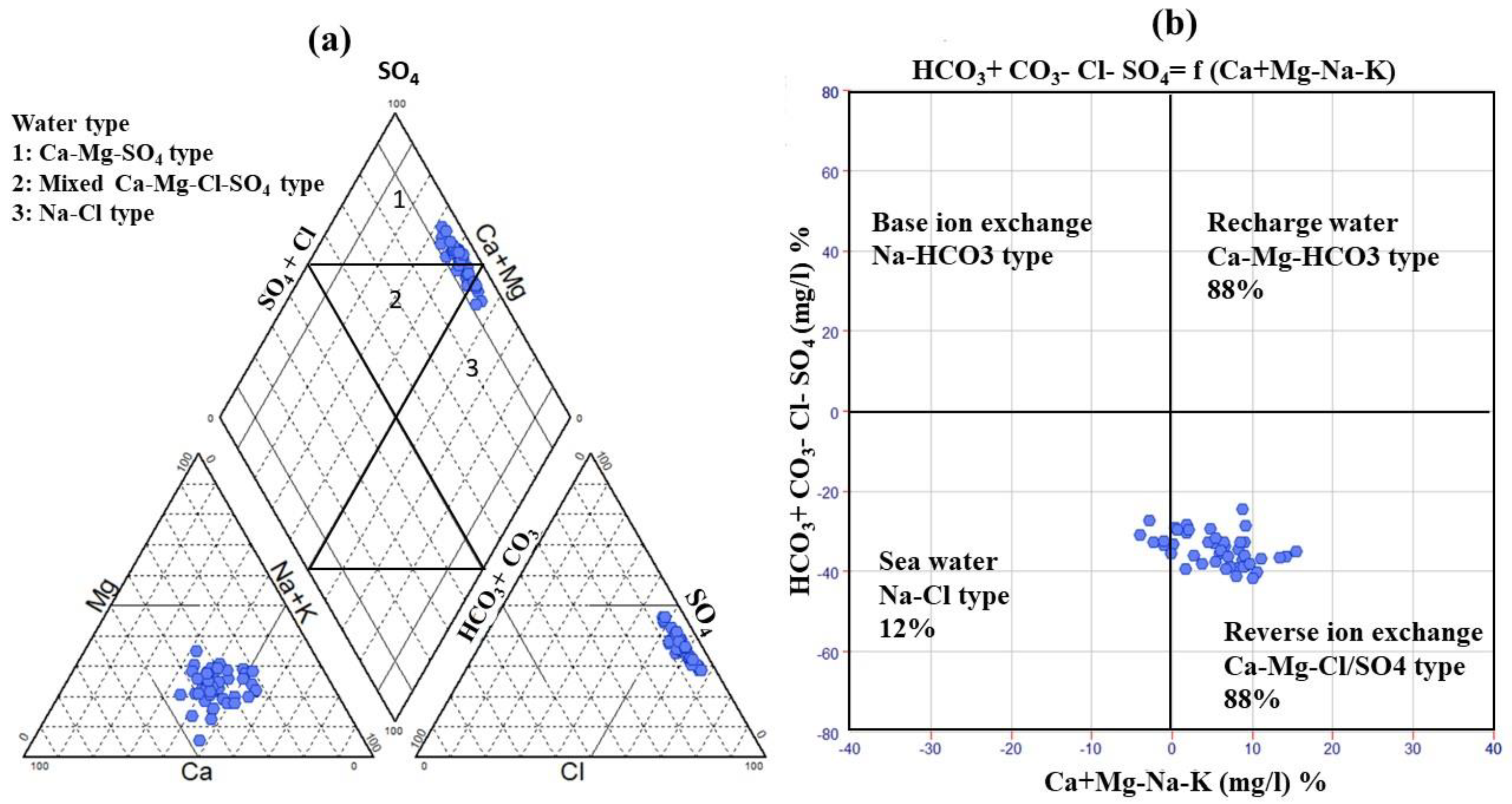
A Piper plot was developed to classify groundwater hydrochemical facies [
50]. The cationic triangle showed that 15.5% of all of the collected samples (south of El-Oued and west of Debila) belonged to the Na
+ + K
+ class, while the remaining were in the nondominant class. In the anionic triangle, Cl
− was the dominant class in 93.3% of the samples, while three water samples in the Robbah, Mih-Ouensan, and west Debila areas were in a nondominant class. In the Piper diagram’s diamond shape, the groundwater samples of the CT aquifer are divided into three main hydrochemical facies (
Figure 5a). Approximately 31 samples fell within the Ca-Mg-SO
4 water type with permanent hardness owing to reverse ion exchange. The high salinity of the water samples was due to the elevated concentration of chloride and calcium ions, especially in the region of Debila. Six samples from El-Oued and Debila had Na
+-Cl
− facies because evaporation was the primary factor controlling the groundwater chemistry. The remaining were in the mixed Ca
2+-Mg
2+-Cl
− class zone and distributed across Hassi Khalifa, El-Oued, and Debila. A Chadha diagram was applied to verify the main dominant geochemical process controlling the groundwater chemistry in the current study [
56]. Approximately 88% of the samples were in the reverse ion exchange zone. Due to the evaporation process, 12% of the samples fell in the field of seawater and was distributed in Debila, Hassi-Khalifa, and Trifaoui (
Figure 5b).
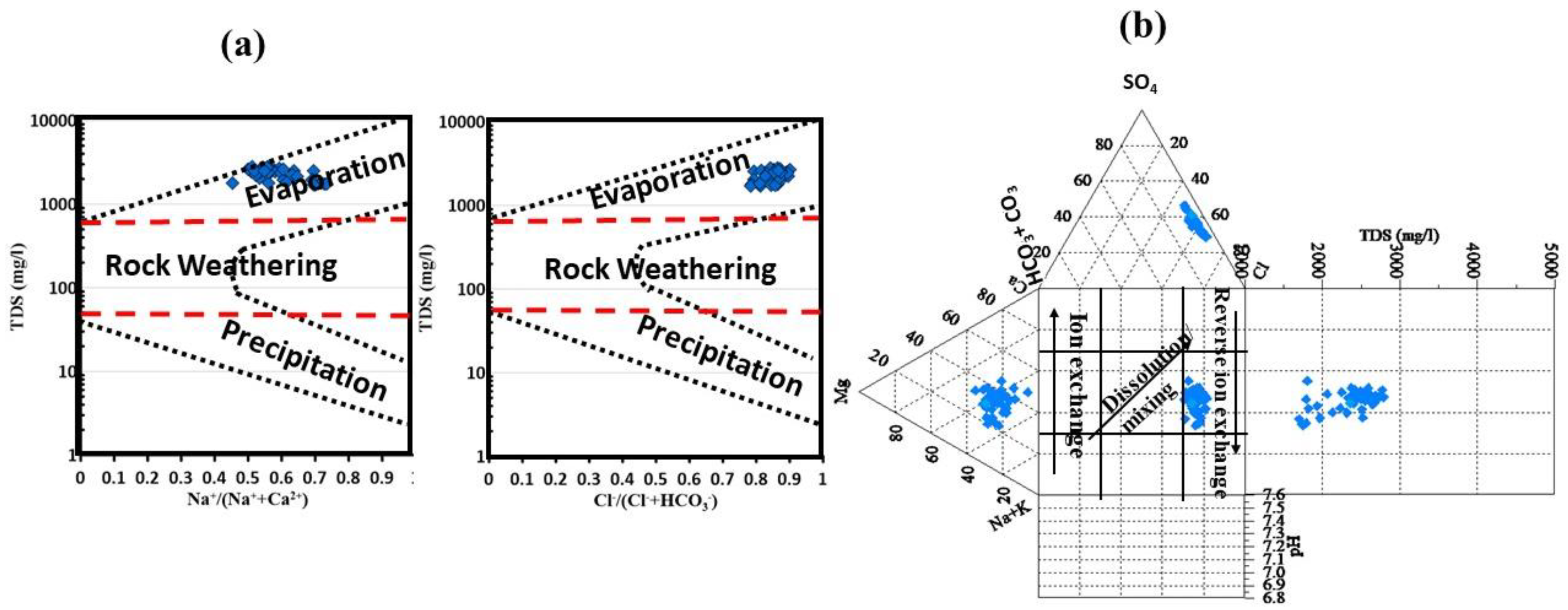
By applying the Gibbs plot to understand the effects of the various mechanisms that control the water chemistry, the diagram was classified into three fundamental zones (
Figure 6a). The first zone is predominately precipitation that has low TDS and a high ratio of Na
+/(Na
+ + Ca
2+) and Cl
−/(Cl
− + HCO
3−). The second domain is distinguished by medium TDS and the abovementioned cation/anion ratio, which represents rock weathering. The evaporation/crystallization domain in the upper half of the Gibbs diagram with extremely high TDS is the last mechanism [
51].
The diagram showed that the groundwater of the CT aquifer was controlled by the evaporation/crystallization process. The water started to precipitate the oversaturated minerals with increasing TDS, and reverse ion exchange can play a significant factor controlling the groundwater chemistry. A Durov diagram, which connects pH, TDS, and major ions, has been utilized as a visualization technique in hydrogeology by various researchers [
57]. The Durov diagram can explain three major processes: mixing/dissolution, ion exchange, and reverse ion exchange (
Figure 6b). With a TDS greater than 1500 mg/L, all of the samples fell within the reverse ion exchange zone, proving the previous statistical explanation.
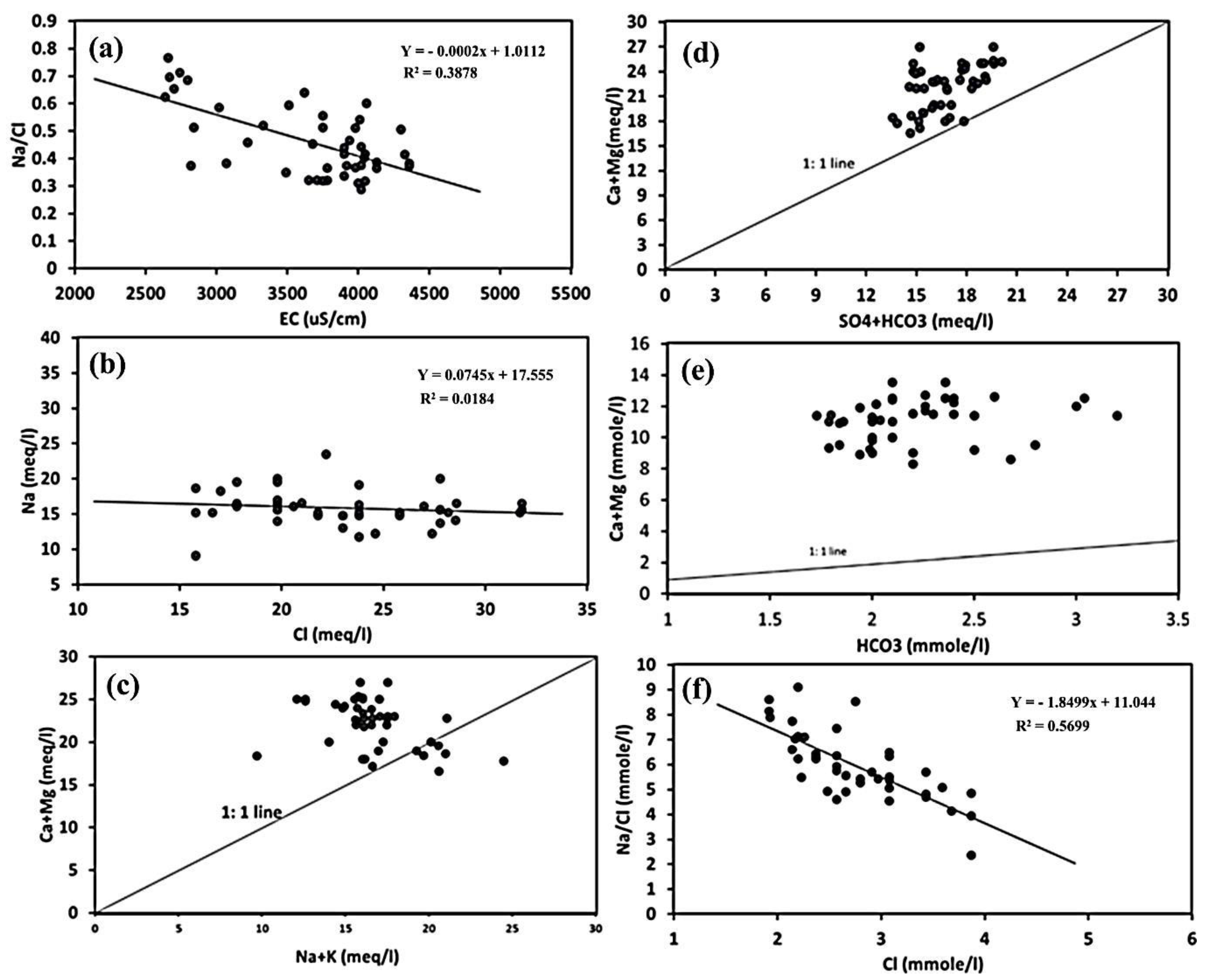
The statistical analysis was utilized to illustrate the main processes governing the chemistry of the groundwater in Souf Valley using the ratios and relationships between the major ions (
Figure 7). The effect of the evaporation process in the CT aquifer can be explained using the graphical relationship between the Na
+/Cl
− ratio and the EC [
58]. The Na
+/Cl
− ratio declined with the increase in the value of the EC as a result of the Na ion depletion caused by reverse ion exchange (
Figure 7a). A Chadha diagram and various ionic plots were used to verify the reverse ion exchange effect on the water chemistry of the CT aquifer. The linearity of the relationship of Cl
− and Na
+ demonstrated the imbalance between the two ions, as only a few groundwater samples fell on a 1:1 line graph because of a typical source (halite dissolution) (
Figure 7b). The majority of the collected samples were scattered beneath the 1:1 line graph due to the fact of chloride enrichment, which is evidence of different sources of chloride ion or the removal of sodium ion from the groundwater.
Anthropogenic activities, including the drainage of excess irrigation water from cropland and waste disposal [
59,
60] or the atmospheric deposition of Cl
− [
61], can cause elevated chloride concentrations. If the Na
+/Cl
− ratio is higher than one, weathering of silicate minerals could be a significant factor [
62], but from the current results of the water samples, the ratio was less than one for all of the samples due to the lack of silicate weathering. The Ca
2+ + Mg
2+ versus Na
+ + K
+ relationship revealed that the samples of the water were categorized into three groups, and the majority of the collected samples overlie the 1:1 line graph (
Figure 7c), three samples crossed the line (1:1 line), and five samples were scattered under the line. The abundance of Mg
2+ and Ca
2+ ions over K
+ and Na
+ ions in the majority of the water samples indicates that sodium ions were replaced by Ca
2+ and Mg
2+ via the direct ion exchange process [
63].
The linear relationship between the HCO
3− + SO
42− and Ca
2+ + Mg
2+ ions (
Figure 7d) revealed that most of the collected samples overlay the 1:1 line, reflecting a reverse ion exchange process. Due to the gypsum/calcite/dolomite dissolution, one sample fell on the 1:1 line graph. Reverse ion exchange is a main reason for the greater abundance of Ca
2+ + Mg
2+ over HCO
3− + SO
42− [
64]. The Ca
2+ + Mg
2+/HCO
3− ratio could clarify the Ca
2+ and Mg
2+ source in the groundwater of the CT aquifer (
Figure 7e). If the value of Ca
2+ + Mg
2+/HCO
3− ratio was near 0.5, the magnesium and calcium ions would be derived mainly from the silicate and carbonate mineral weathering [
65]. If the ratio was <0.5, the bicarbonate enrichment and/or ion exchange could be the significant factor for the magnesium and calcium ions’ depletion. All of the water samples had a ratio >0.5. Because of the slightly alkaline condition of the groundwater, the depletion of HCO
3− as a cause of this high ratio value was neglected, leaving only the reverse ion exchange as the main process accounting for all of the samples overlaying the 1:1 line (ratio = 0.5) [
66].
The value of the Ca
2+ + Mg
2+/HCO
3− ratio could be useful to determine the groundwater recharge and its meteoric nature. If this ratio is less <1, the water is meteoric and there is recharge for the aquifer [
67]. All of the collected samples of the CT aquifer had a remarkably large ratio, varying from 3.2 to 6.5, indicating the lack of meteoric nature as well as indicating the recharge of the groundwater. The linear graph between Na
+/Cl
− and Cl
− (
Figure 7f) shows an inverse association, suggesting that calcium and magnesium replaced sodium caused by halite dissolution in the CT aquifer matrix (clay minerals) [
64].
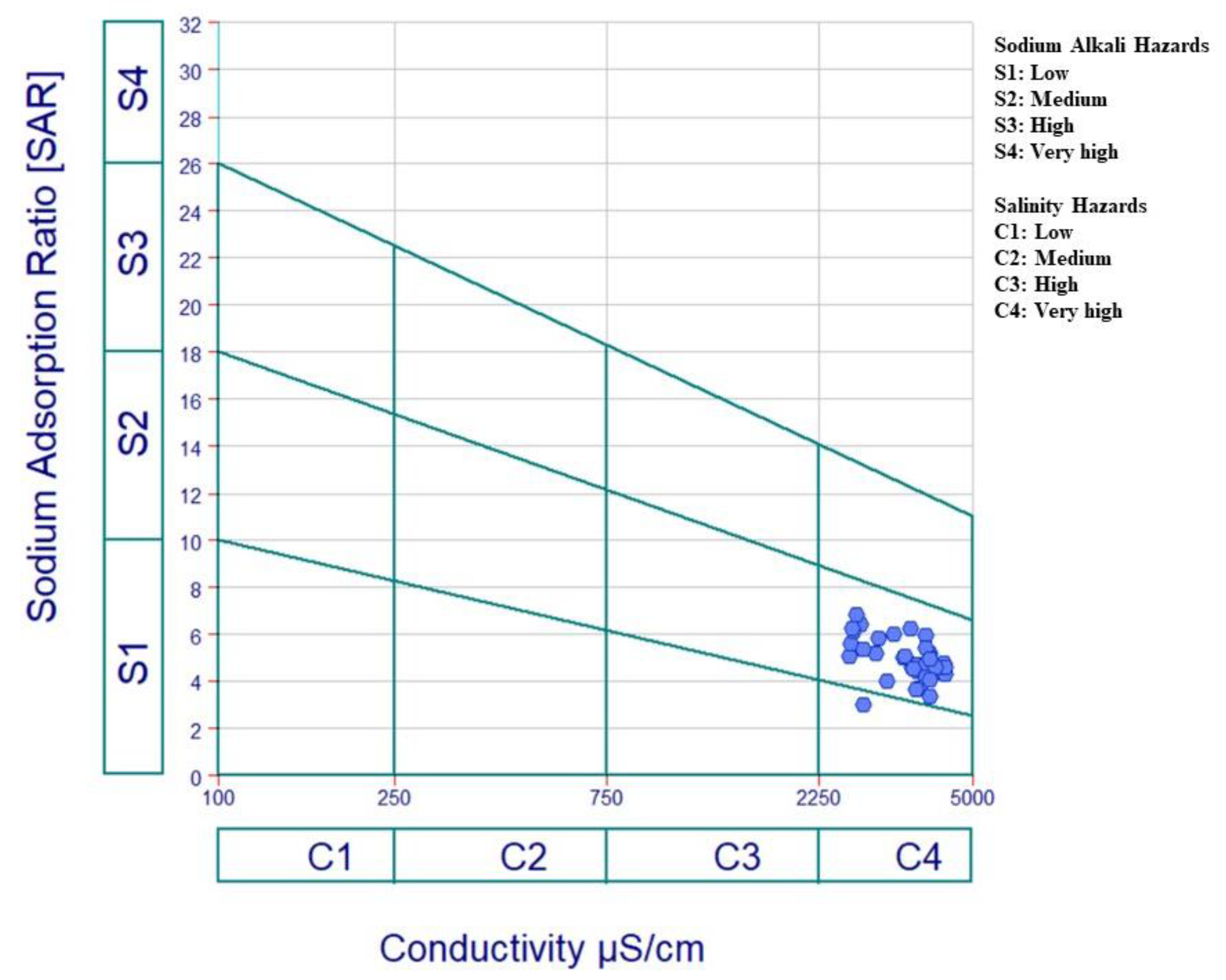
3.11. Residual Sodium Carbonate (RSC)
Another aspect influencing irrigation water quality is excessive carbonates and bicarbonates in relation to Ca
+2 and Mg
+2 ions, which can reduce irrigation water quality by precipitating alkali metals, primarily Mg
+2 and Ca
+2. The SAR value and sodium ion concentrations may both rise as a result of the precipitation of Ca
+2 and Mg
+2 as carbonate minerals. [
35]. High RSC has the potential to deteriorate the soil’s physical qualities by causing the dissociation of organic matter, which eventually results in a black stain on the soil’s surface after drying [
80,
81].
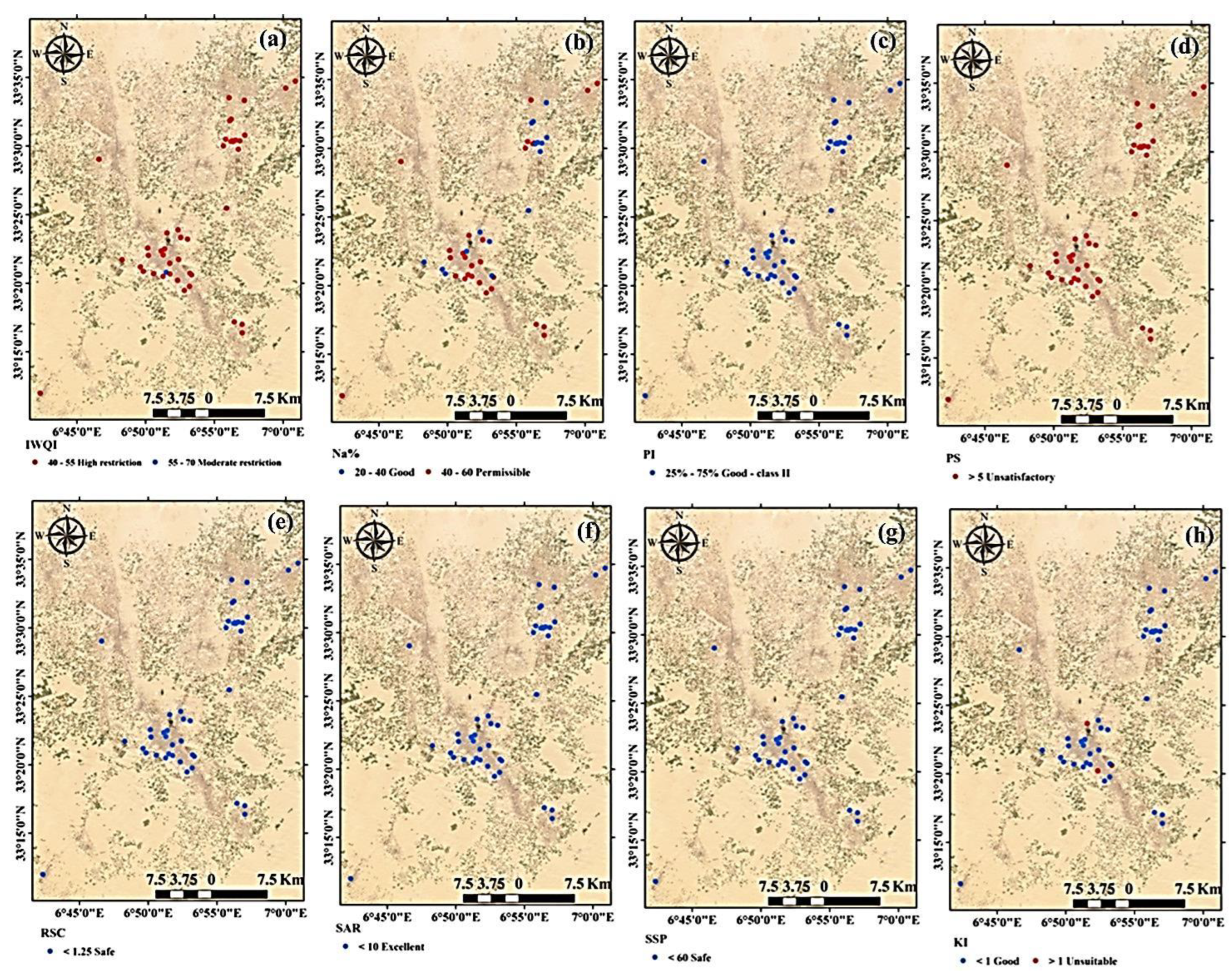
The RSC was computed to determine the possible precipitation of Ca
2+ and Mg
2+ on the particles of the soil’s surface. The values of the RSC index in groundwater is reported to be high in areas that are dry to semi-dry, causing soil sodification and soil salinization [
82]. According to the RSC values, the groundwater was divided into three categories (
Figure 8h). Irrigation water with an RSC greater than 2.5 is not appropriate for irrigation, whereas water with an RSC less than 1.25 is good, and water with an RSC that ranges from 1.25 and 2.5 is doubtful for use in irrigation [
35]. In the current study, all groundwater samples had an RSC value < 1.25, demonstrating that the groundwater was suitable and safe for irrigation uses (
Figure 8h).
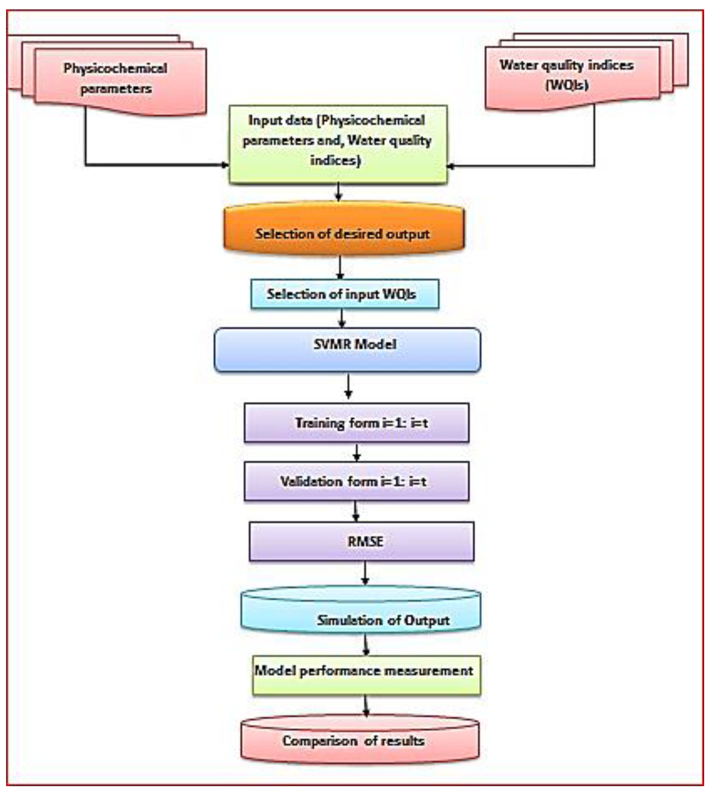
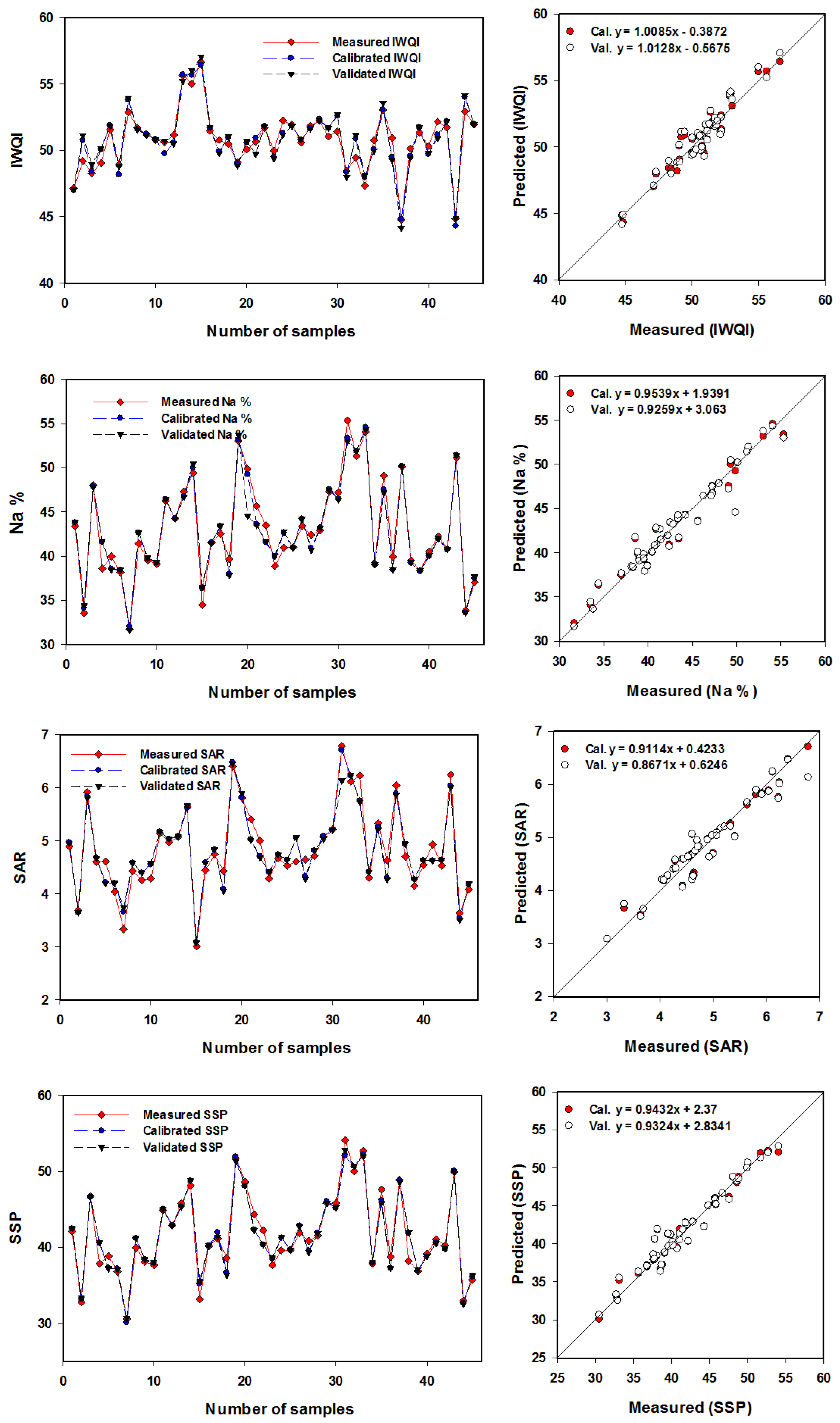
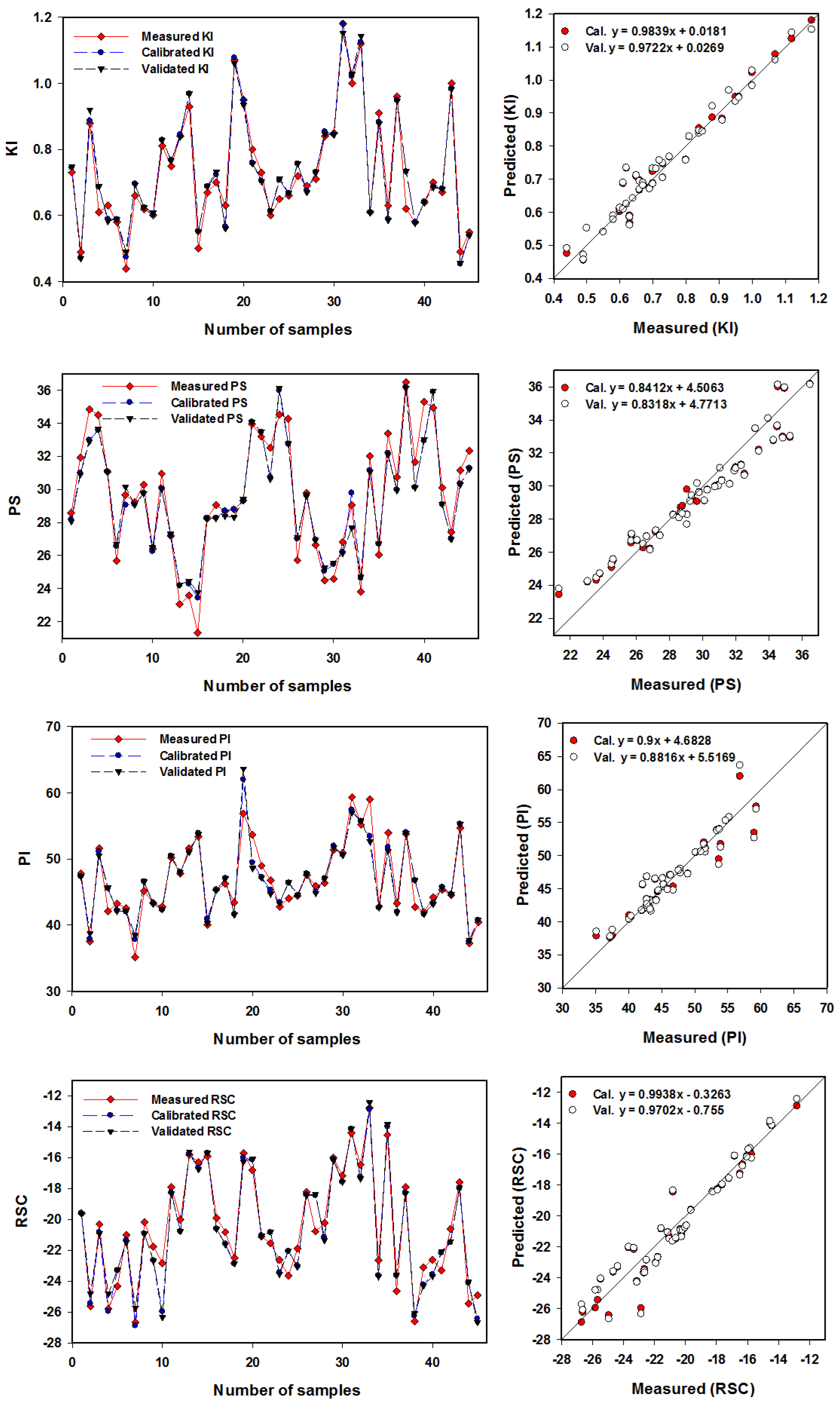
3.12. Performance of the Support Vector Machine Regression Based on Physicochemical Parameters for Predicting the Irrigation Water Quality Indices
Several researchers have investigated methods for reducing the subjectivity of established water quality index technology, which has been proven to be a more accurate and precise essential tool for reliable weighing systems by assigning weights to critical ions based on entropy [
83]. Water quality research, on the other hand, necessarily requires a significant amount of data collection, laboratory analysis, data management, and testing [
84]. As a consequence of the computation’s subjectivity, the WQIs’ interpretation of the results contained inconsistencies. It is possible to identify a subset of features that have high predictive and discriminative potential using methods for feature selection based on models [
85]. By minimizing overfitting and eliminating pointless features, this strategy can enhance the model performance. The original feature representation should be kept, because it provides a number of benefits on top of improving the interpretability [
86]. In the disciplines of modeling and prediction, there is an increasing need for feature selection algorithms [
87].
Mathematical techniques can be used to estimate the IWQIs of water sites with accuracy. These techniques, however, are difficult to apply to evaluate IWQIs, because they require a number of mathematical equations to convert a sizable amount of data on water characterization into a single value that characterizes the water quality levels and reflects the overall water quality level. This study evaluated the SVMR model to predict the IWQIs based on the numerous response factors of the chemical parameters. The SVMR model was used in this work to anticipate the IWQIs based on various parameters, as shown in
Table 6, because it is fast and does not require several more steps to construct the IWQIs.
The SVMR model was utilized to more accurately assess eight IWQIs relying on the R
2 and RMSE values (
Table 6) and the slope (
Figure 10 and
Figure 11). With R
2 values ranging from 0.90 to 0.97, the SVMR model achieved robust estimates for eight IWQIs in the Cal. datasets. Moreover, the SVMR model produced accurate estimations for eight IWQIs in the Val. datasets, with the R
2 ranging from 0.88 to 0.95. The validation model’s RMSE values for eight IWQIs, including IWQI, Na%, SAR, SSP, KI, PS, PI, and RSC, as shown in
Table 6, were 0.92, 1.37, 0.27, 1.42, 0.05, 1.20, 2.09, and 2.09, respectively.
Figure 10 and
Figure 11 show the SVMR based association of the eight IWQIs. Furthermore, these figures showed a reasonable slope of the linear relationship between the predicted and measured validation model values for every index, with IWQI having the highest slope (1.0128) and PS having the lowest slope (0.8318). There was no overfitting or underfitting in the datasets used to measure, calibrate, and validate the SVMR models of the eight IWQIs. As an outcome, the models applied in this study had sufficient accuracy and performed well when forecasting the IWQIs. These findings are consistent with those in [
88], which found that the principal component regression produced precise and powerful models that predicted the IWQIs, with R
2 values ranging from 0.48 to 0.99. Based on four parameters, including temperature, turbidity, pH, and TDS, Ahmed et al. [
89] discovered that supervised machine learning with multiple linear regression could be used to estimate the water quality index of surface waters with an R
2 value of 0.66. Multiple linear regression models with R
2 values that reached 0.64 were discovered by Chen and Liu [
90] to be useful for estimating water quality indicators, such as dissolved oxygen, total phosphorus, and chlorophyll disc depth.


 ,
, 


