Predicting Flood Frequency with the LH-Moments Method: A Case Study of Prigor River, Romania

Anghel, Cristian Gabriel; Ilinca, Cornel

doi:10.3390/w15112077

Open AccessArticle

Predicting Flood Frequency with the LH-Moments Method: A Case Study of Prigor River, Romania

by

Cristian Gabriel Anghel

and

Cornel Ilinca

^*

Faculty of Hydrotechnics, Technical University of Civil Engineering Bucharest, Lacul Tei, nr.122−124, 020396 Bucharest, Romania

^*

Author to whom correspondence should be addressed.

Water 2023, 15(11), 2077; https://doi.org/10.3390/w15112077

Submission received: 5 May 2023 / Revised: 21 May 2023 / Accepted: 28 May 2023 / Published: 30 May 2023

(This article belongs to the Special Issue Hydrological Extreme Events and Climate Changes)

Download

Browse Figures

Versions Notes

Abstract

:

The higher-order linear moments (LH-moments) method is one of the most commonly used methods for estimating the parameters of probability distributions in flood frequency analysis without sample censoring. This article presents the relationships necessary to estimate the parameters for eight probability distributions used in flood frequency analysis. Eight probability distributions of three parameters using first- and second-order LH-moments are presented, namely the Pearson V distribution, the CHI distribution, the inverse CHI distribution, the Wilson–Hilferty distribution, the Pseudo-Weibull distribution, the Log-normal distribution, the generalized Pareto Type I distribution and the Fréchet distribution. The exact and approximate relations for parameter estimation are presented, as are the exact and approximate relations for estimating the frequency factor specific to each method. In addition, the exact and approximate relationships of variation in the LH-skewness–LH-kurtosis are presented, as is the variation diagram of these statistical indicators. To numerically represent the analyzed distributions, a flood frequency analysis case study using the annual maximum series was carried out for the Prigor River. The analysis is presented compared to the linear moments (L-moments) method, which is the method that is intended to be used in the development of a new norm in Romania for determining the maximum flows. For the Prigor River, the most fit distributions are the Pseudo-Weibull and the generalized Pareto Type I for the linear moments method and the CHI and the Wilson–Hilferty distributions for the first higher-order linear moments method. The performance was evaluated using linear and higher-order linear moment values and diagrams.

Keywords:

frequency analysis; Pearson; Weibull; Fréchet; chi; Pareto; parameters; approximate form; linear moments; higher-order linear moments

1. Introduction

Since 1996, the higher-order linear moments (LH-moments) method for estimating the parameters of probability distributions in flood frequency analysis has become one of the most popular estimation methods without sample censoring.

This method was introduced by Wang [1] for flood frequency analysis using the Annual Maximum Series (AMS), a generalization of the linear moments method [2,3,4,5] “based on linear combinations of higher-orders statistics, introduced for characterizing the upper part of distributions and larger events in data” [1] up to the fourth order. The method fulfills the so-called “separation effect” [4,6], namely assigning a reduced importance to the lower maximum values, which are not always “floods”. This represents the main disadvantage of using the maximum annual series, which is made up of maximum flow values characteristic of each year.

In hydrology, the LH-moments method has been generally applied for low-flow frequency analysis [7], flood frequency analysis [1,8,9,10], regional flood frequency analysis [11,12,13,14] and frequency analysis of the annual maximum rainfall series [15,16,17].

In this article, only the first two LH-moments are analyzed, and we have formulated the LH-moments for all the analyzed distributions, i.e., the Pearson V (PV) distribution, the CHI distribution, the CHI inverse distribution (ICH), the Wilson–Hilferty distribution (WH), the Pseudo-Weibull distribution (PW), the Log-normal distribution (LN3), the generalized Pareto Type I distribution (PGI) and the Fréchet distribution (FR).

In recent research [18,19,20,21] for these distributions, new mathematical elements are presented regarding their easy applicability in flood frequency analysis, such as the exact and approximate relations for estimating the parameters of the distributions and the frequency factors using the method of ordinary moments and the method of linear moments.

The results obtained from the analyzed case study are presented compared to the L-moments method, because these methods are intended to be used in the new regulations in Romania regarding flood frequency analysis. These methods are much more stable parameter estimation methods and less subject to bias [2,3,4,5,22,23] compared to other parameter estimation methods, especially for small lengths of observed data. In recent years, based on the work of Anghel and Ilinca [20], it has been observed that the L-moments method requires certain corrections of the statistical indicators, which can be achieved using the least-squares method. Gaume [23] also mentions that “the L−moments are less sensitive to sampling variability, but parameters and quantiles are related to the moments by nonlinear functions. The advantage of the lower variance of the L-moments may be lost due to this nonlinear transformation…”. The same principle is applied to LH-moments.

The main purpose of the article is to present all the elements necessary to apply these distributions using the first and second LH-moments method, which is a method that is intended to be implemented in a future normative regarding the determination of maximum flows in Romania. Being a method that achieves the effect of separating the lower maximum flows from the higher ones from the annual series of maximum flows, this can represent an alternative to the frequency analysis that uses the partial series. It also represents a parameter estimation method whose statistical indicators (expected value, L-coefficient of variation, L-skewness, L-kurtosis) can be used to achieve regionalization.

The exact and approximate relations for estimating the parameters of these probability distributions using the L-moments method were also presented in previous research [19,20,21].

In this article, the new elements that are presented are the exact and approximate relationships for parameter estimation, the expression of the inverse functions with the frequency factor, the exact and approximate relationships of the frequency factors, the diagram and the variation relationships of LH-skewness and LH−kurtosis, the confidence interval using the frequency factors and Chow’s relationship [3,18,24,25,26].

All these novelty elements for the distributions presented in Table 1 will help hydrology researchers better understand and easily apply these distributions using LH-moments.

Based on the work of Anghel and Ilinca [19,20,21], the inverse function is expressed using the frequency factor for both methods. Table A1 in Appendix B shows the frequency factors of the analyzed distributions for the L-moments and LH-moments methods. Other important novelty elements are the relationships and the LH-skewness (

τ_{H 3}

)–LH-kurtosis (

τ_{H 4}

) variation diagrams for the analyzed distributions, presented in Appendix C and Appendix D.

The parameter approximation relations are necessary because, for some probability distributions, it is necessary to solve nonlinear systems of equations, which leads to some difficulties. The relative errors of parameter estimation are between 10⁻² and 10⁻⁴.

Moreover, for a fast but still accurate calculation, the approximation relations of the frequency factors are presented for both methods for the most common exceedance probabilities in flood frequency analysis (see Appendix E, Appendix F, Appendix G and Appendix H).

All the analyzed distributions and methods presented are applied for flood frequency analysis using the Annual Maximum Series (AMS) for the Prigor River.

The best model is chosen based on the linear moments and the higher-order linear moment values and diagrams.

Indicatively, the values of the relative mean error (RME) and the relative absolute error (RAE) indicators [3] are presented, but it is known that they only properly evaluate the probability area of the observed values.

The article is organized as follows: In Section 2.1, the inverse functions of the probability distributions are presented. In Section 2.2, the relations for the exact calculation and the approximate relations for determining the parameters of the distributions are presented. In Section 3, these distributions and methods are applied for the flood frequency analysis using the AMS for the Prigor River. The results, discussion and conclusions are presented in Section 4, Section 5 and Section 6.

2. Methods

The methods for estimating the parameters of probability distributions analyzed in this article are the L-moments method and the LH-moments method, representing two of the most commonly used parameter estimation methods.

The analysis consists in determining the maximum flows on the Prigor River using the series of annual maximum flows applying the Pearson V, CHI, inverse CHI, Wilson–Hilferty, Pseudo-Weibull, Log-normal, generalized Pareto Type I and Fréchet distributions, as well as the L-moments methods and the LH-moments for parameter estimation.

The derivations of sample L-moments and LH-moments are realized according to formal studies [1,2,3,4,5].

2.1. Probability Distributions

Being two methods based exclusively on the inverse function of the probability distribution, Table 2 only presents the quantile function,

x (p)

, for the analyzed distributions [18,19,20,21,27].

The probability density function

f (x)

and the complementary cumulative distribution function

F (x)

for the analyzed distributions are presented in Appendix I.

All the predefined functions are detailed in Appendix K.

2.2. Parameter Estimation

This section presents the exact and approximate relations for estimating the parameters of the analyzed probability distributions for the first-order LH-moments method. The exact and approximate relations for estimating the parameters of the distributions analyzed for the second-order LH-moments are presented in Appendix A.

The relative errors characterizing the approximate estimates depend only on the values of the statistical indicator LH-skewness (

|τ_{H 3}|

), which are always between 0 and 1.

The relationships for estimating the parameters using the L-moments method, as well as their applicability in flood frequency analysis, were presented in previous research [18,19,20,21].

2.2.1. Pearson V (PV)

For the LH-moments method, the parameters are calculated numerically (definite integrals) using the inverse function, but an approximate form of parameter estimation can be adopted. The shape parameter

α

can be evaluated numerically with the following approximate forms, depending on LH-skewness (

τ_{H 3}

):

if $0.12 < |τ_{H 3}| \leq 0.5$ :

α = \exp (\begin{array}{l} 33 . 1789157 + 210 . 1051405 \cdot \ln (|τ_{H 3}|) + 585 . 9500753 \cdot \ln {(|τ_{H 3}|)}^{2} + \\ 915 . 6647285 \cdot \ln {(|τ_{H 3}|)}^{3} + 883 . 3738137 \cdot \ln {(|τ_{H 3}|)}^{4} + 539 . 3747506 \cdot \ln {(|τ_{H 3}|)}^{5} + \\ 204 . 1998415 \cdot \ln {(|τ_{H 3}|)}^{6} + 43 . 9583804 \cdot \ln {(|τ_{H 3}|)}^{7} + 4 . 1340485 \cdot \ln {(|τ_{H 3}|)}^{8} \end{array})

(1)

if $0.5 < |τ_{H 3}| \leq 0.89$ :

α = \exp (0 . 6283077 - 0 . 5109263 \cdot \ln (|τ_{H 3}|) + 0 . 2918709 \cdot \ln {(|τ_{H 3}|)}^{2} - 0 . 2992959 \cdot \ln {(|τ_{H 3}|)}^{3})

(2)

The scale parameter

β

and the position parameter

γ

are determined by the following expressions:

β = \frac{L_{H 2}}{\frac{3}{2} \cdot z_{1}}

(3)

γ = L_{H 1} - 2 \cdot β \cdot z_{2}

(4)

where

z_{1} = \int_{0}^{1} \frac{1}{q g a m m a (1 - p, α - 1)} \cdot (3 \cdot p^{2} - 2 \cdot p) \cdot d p

, which can be approximated with the following equation:

z_{1} = \frac{0 . 11655082 + 0 . 03060228 \cdot α - 0 . 00076384 \cdot α^{2} + 0 . 0000079 \cdot α^{3}}{1 - 1 . 179253 \cdot α + 0 . 33961387 \cdot α^{2}}

(5)

and

z_{2} = \int_{0}^{1} \frac{1}{q g a m m a (1 - p, α - 1)} \cdot p \cdot d p

, which can be approximated with the following equation:

z_{2} = \frac{- 0 . 19533553 + 0 . 22880951 \cdot α - 0 . 00122785 \cdot α^{2} + 0 . 00001518 \cdot α^{3}}{1 - 1 . 26076825 \cdot α + 0 . 38037518 \cdot α^{2}}

(6)

L_{H 1}

and

L_{H 2}

represent the first two LH-moments.

2.2.2. CHI

For the LH-moments method, the parameters are calculated numerically (definite integrals) using the inverse function.

The shape parameter

α

can be evaluated numerically with the following approximate forms, depending on LH-skewness (

τ_{H 3}

):

if $0.12 < |τ_{H 3}| \leq 0.35$ :

α = \exp (\begin{array}{l} - 16694 . 76115 - 100768 . 156 \cdot \ln (|τ_{H 3}|) - 268451 . 17727 \cdot \ln {(|τ_{H 3}|)}^{2} - \\ 414276 . 35912 \cdot \ln {(|τ_{H 3}|)}^{3} - 408164 . 33969 \cdot \ln {(|τ_{H 3}|)}^{4} - \\ 266288 . 40807 \cdot \ln {(|τ_{H 3}|)}^{5} - 115056 . 13395 \cdot \ln {(|τ_{H 3}|)}^{6} - 31753 . 48498 \cdot \ln {(|τ_{H 3}|)}^{7} - \\ 5080 . 28503 \cdot \ln {(|τ_{H 3}|)}^{8} - 359 . 09072 \cdot \ln {(|τ_{H 3}|)}^{9} \end{array})

(7)

if $0.35 < |τ_{H 3}| \leq 0.86$ :

α = \frac{\begin{array}{l} 698 . 77925304 - 2242 . 91013463 \cdot |τ_{H 3}| + 3940 . 25464468 \cdot τ_{H 3}^{2} - \\ 3816 . 83817207 \cdot τ_{H 3}^{3} + 1382 . 96600663 \cdot τ_{H 3}^{4} \end{array}}{1 + 1919 . 25596802 \cdot |τ_{H 3}|}

(8)

The scale parameter

β

and the position parameter

γ

are determined by the following expressions:

β = \frac{L_{H 2}}{\frac{3}{2} \cdot z_{1}}

(9)

γ = L_{H 1} - 2 \cdot β \cdot z_{2}

(10)

where

z_{1} = \int_{0}^{1} \sqrt{2 \cdot q g a m m a (p, \frac{α}{3})} \cdot (3 \cdot p^{2} - 2 \cdot p) \cdot d p

, which can be approximated with the following equation:

z_{1} = \exp (\begin{array}{l} - 1 . 6193192 + 0 . 0911325 \cdot \ln (α) - 0 . 0732734 \cdot \ln {(α)}^{2} + \\ 0 . 0210155 \cdot \ln {(α)}^{3} - 0 . 0002631 \cdot \ln {(α)}^{4} - \\ 0 . 0007313 \cdot \ln {(α)}^{5} + 0 . 0000303 \cdot \ln {(α)}^{6} + 0 . 0000107 \cdot \ln {(α)}^{7} \end{array})

(11)

and

z_{2} = \int_{0}^{1} \sqrt{2 \cdot q g a m m a (p, \frac{α}{3})} \cdot p \cdot d p

, which can be approximated with the following equation:

z_{2} = \exp (\begin{array}{l} - 0 . 5729973 + 0 . 5558033 \cdot \ln (α) - 0 . 0535962 \cdot \ln {(α)}^{2} + \\ 0 . 0108076 \cdot \ln {(α)}^{3} + 0 . 000948 \cdot \ln {(α)}^{4} - 0 . 0004607 \cdot \ln {(α)}^{5} + \\ 0 . 0000087 \cdot \ln {(α)}^{6} + 0 . 0000083 \cdot \ln {(α)}^{7} \end{array})

(12)

2.2.3. Inverse CHI (ICH)

For the LH-moments method, the parameters are calculated numerically (definite integrals) using the inverse function.

The shape parameter

α

can be evaluated numerically with the following approximate forms, depending on LH-skewness (

τ_{H 3}

):

if $0.13 < |τ_{H 3}| \leq \frac{1}{3}$ :

α = \exp (\begin{array}{l} - 61180 . 3132156 - 366053 . 2214846 \cdot \ln (|τ_{H 3}|) - 967907 . 6881457 \cdot \ln {(|τ_{H 3}|)}^{2} - \\ 1484555 . 793998 \cdot \ln {(|τ_{H 3}|)}^{3} - 1455630 . 615952 \cdot \ln {(|τ_{H 3}|)}^{4} - \\ 946282 . 7853778 \cdot \ln {(|τ_{H 3}|)}^{5} - 407886 . 238361 \cdot \ln {(|τ_{H 3}|)}^{6} - 112421 . 4415708 \cdot \ln {(|τ_{H 3}|)}^{7} - \\ 17980 . 252856 \cdot \ln {(|τ_{H 3}|)}^{8} - 1271 . 5300784 \cdot \ln {(|τ_{H 3}|)}^{9} \end{array})

(13)

if $\frac{1}{3} < |τ_{H 3}| \leq 0.86$ :

α = \exp (\begin{array}{l} - 0 . 8215758 - 1 . 0358243 \cdot \ln (|τ_{H 3}|) + 0 . 495645 \cdot \ln {(|τ_{H 3}|)}^{2} + \\ 0 . 0935625 \cdot \ln {(|τ_{H 3}|)}^{3} + 0 . 1199457 \cdot \ln {(|τ_{H 3}|)}^{4} \end{array})

(14)

The scale parameter

β

and the position parameter

γ

are determined by the following expressions:

β = \frac{L_{H 2}}{\frac{3}{2} \cdot z_{1}}

(15)

γ = L_{H 1} - 2 \cdot β \cdot z_{2}

(16)

where

z_{1} = \int_{0}^{1} \frac{1}{\sqrt{q g a m m a (1 - p, α)}} \cdot (3 \cdot p^{2} - 2 \cdot p) \cdot d p

, which can be approximated with the following equation:

z_{1} = \exp (\begin{array}{l} - 0 . 564274128 - 2 . 882522149 \cdot \ln (α) + 2 . 255841146 \cdot \ln {(α)}^{2} - \\ 2 . 247784696 \cdot \ln {(α)}^{3} + 1 . 499774603 \cdot \ln {(α)}^{4} - \\ 0 . 632746529 \cdot \ln {(α)}^{5} + 0 . 166600377 \cdot \ln {(α)}^{6} - \\ 0 . 026534223 \cdot \ln {(α)}^{7} + 0 . 002338161 \cdot \ln {(α)}^{8} - 0 . 000087492 \cdot \ln {(α)}^{9} \end{array})

(17)

and

z_{2} = \int_{0}^{1} \frac{1}{\sqrt{q g a m m a (1 - p, α)}} \cdot p \cdot d p

, which can be approximated with the following equation:

z_{2} = \exp (\begin{array}{l} 0 . 2300873 - 1 . 8414555 \cdot \ln (α) + 1 . 8519728 \cdot \ln {(α)}^{2} - \\ 2 . 2245978 \cdot \ln {(α)}^{3} + 1 . 8378594 \cdot \ln {(α)}^{4} - 0 . 9868348 \cdot \ln {(α)}^{5} + \\ 0 . 343659 \cdot \ln {(α)}^{6} - 0 . 0770063 \cdot \ln {(α)}^{7} + 0 . 0107105 \cdot \ln {(α)}^{8} - \\ 0 . 0008412 \cdot \ln {(α)}^{9} + 0 . 0000285 \cdot \ln {(α)}^{10} \end{array})

(18)

2.2.4. Wilson–Hilferty (WH)

For the LH-moments method, the parameters are calculated numerically (definite integrals) using the inverse function. The shape parameter

α

can be evaluated numerically with the following approximate forms, depending on LH-skewness (

τ_{H 3}

):

if $0.12 < |τ_{H 3}| \leq 0.35$ :

α = \exp (\begin{array}{l} 57 . 509799785 + 253 . 518955488 \cdot \ln (|τ_{H 3}|) + 436 . 520035507 \cdot \ln {(|τ_{H 3}|)}^{2} + \\ 394 . 289299803 \cdot \ln {(|τ_{H 3}|)}^{3} + 198 . 423841713 \cdot \ln {(|τ_{H 3}|)}^{4} + \\ 52 . 828181707 \cdot \ln {(|τ_{H 3}|)}^{5} + 5 . 824373504 \cdot \ln {(|τ_{H 3}|)}^{6} \end{array})

(19)

if $0.35 < |τ_{H 3}| \leq 0.86$ :

α = \frac{273 . 6242257 - 98 . 24031624 \cdot |τ_{H 3}| - 235 . 34533957 \cdot τ_{H 3}^{2}}{1 + 5141 . 39837304 \cdot |τ_{H 3}| + 2429 . 51377444 \cdot τ_{H 3}^{2}}

(20)

The scale parameter

β

and the position parameter

γ

are determined by the following expressions:

β = \frac{L_{H 2}}{\frac{3}{2} \cdot z_{1}}

(21)

γ = L_{H 1} - 2 \cdot β \cdot z_{2}

(22)

where

z_{1} = \int_{0}^{1} q g a m m a {(p, α)}^{\frac{1}{3}} \cdot (3 \cdot p^{2} - 2 \cdot p) \cdot d p

, which can be approximated with the following equation:

z_{1} = \exp (\begin{array}{l} - 2 . 3478324 - 0 . 1189079 \cdot \ln (α) + 0 . 0572596 \cdot \ln {(α)}^{2} + \\ 0 . 0450416 \cdot \ln {(α)}^{3} - 0 . 0035155 \cdot \ln {(α)}^{4} - \\ 0 . 0020952 \cdot \ln {(α)}^{5} - 0 . 0001603 \cdot \ln {(α)}^{6} \end{array})

(23)

and

z_{2} = \int_{0}^{1} q g a m m a {(p, α)}^{\frac{1}{3}} \cdot p \cdot d p

, which can be approximated with the following equation:

z_{2} = \exp (\begin{array}{l} - 0 . 6136735 + 0 . 3733551 \cdot \ln (α) + 0 . 0145217 \cdot \ln {(α)}^{2} + \\ 0 . 0408459 \cdot \ln {(α)}^{3} + 0 . 0063655 \cdot \ln {(α)}^{4} + 0 . 0001819 \cdot \ln {(α)}^{5} - \\ 0 . 0000152 \cdot \ln {(α)}^{6} \end{array})

(24)

2.2.5. Pseudo-Weibull (PW)

For the LH-moments method, the parameters are calculated numerically (definite integrals) using the inverse function. The shape parameter

α

can be evaluated numerically with the following approximate forms, depending on LH-skewness (

τ_{H 3}

):

α = \exp (\begin{array}{l} - 3 . 8466499 - 9 . 7748142 \cdot \ln (α) - 19 . 6970479 \cdot \ln {(α)}^{2} - \\ 30 . 004269 \cdot \ln {(α)}^{3} - 29 . 1593303 \cdot \ln {(α)}^{4} - 17 . 8271467 \cdot \ln {(α)}^{5} - \\ 6 . 6407414 \cdot \ln {(α)}^{6} - 1 . 3760942 \cdot \ln {(α)}^{7} - 0 . 1215435 \cdot \ln {(α)}^{8} \end{array})

(25)

The scale parameter

β

and the position parameter

γ

are determined by the following expressions:

β = \frac{L_{H 2}}{\frac{3}{2} \cdot z_{1}}

(26)

γ = L_{H 1} - 2 \cdot β \cdot z_{2}

(27)

where

z_{1} = \int_{0}^{1} q g a m m a {(p, \frac{1}{α} + 1)}^{\frac{1}{α}} \cdot (3 \cdot p^{2} - 2 \cdot p) \cdot d p

, which can be approximated with the following equation:

z_{1} = \exp (\begin{array}{l} - 0 . 771576 - 2 . 2235425 \cdot \ln (α) + 1 . 1244123 \cdot \ln {(α)}^{2} - \\ 0 . 5660755 \cdot \ln {(α)}^{3} + 0 . 1614285 \cdot \ln {(α)}^{4} - 0 . 0410233 \cdot \ln {(α)}^{5} + \\ 0 . 0180276 \cdot \ln {(α)}^{6} \end{array})

(28)

and

z_{2} = \int_{0}^{1} q g a m m a {(p, \frac{1}{α} + 1)}^{\frac{1}{α}} \cdot p \cdot d p

, which can be approximated with the following equation:

z_{2} = \exp (\begin{array}{l} 0 . 317018 - 1 . 5848028 \cdot \ln (α) + 1 . 20619 \cdot \ln {(α)}^{2} - \\ 0 . 5676031 \cdot \ln {(α)}^{3} + 0 . 1612407 \cdot \ln {(α)}^{4} - 0 . 0417302 \cdot \ln {(α)}^{5} + \\ 0 . 0179191 \cdot \ln {(α)}^{6} \end{array})

(29)

2.2.6. Log-Normal (LN3)

For the L-moments and LH-moments methods, the parameters are calculated numerically (definite integrals) using the inverse function. The scale parameter

β

can be evaluated numerically with the following approximate forms, depending on LH-skewness (

τ_{H 3}

):

β = \frac{- 0 . 299614774 + 3 . 042079635 \cdot |τ_{3 H}| - 2 . 900801018 \cdot τ_{3 H}^{2}}{1 - 0 . 933093562 \cdot |τ_{3 H}| - 0 . 64009136 \cdot τ_{3 H}^{2} + 0 . 51414951 \cdot {|τ_{3 H}|}^{3}}

(30)

The shape parameter

α

and the position parameter

γ

are determined by the following expressions:

α = \ln (\frac{3}{2} \cdot \frac{L_{H 2}}{z_{1}})

(31)

γ = L_{H 1} - 2 \cdot \exp (α) \cdot z_{2}

(32)

where

z_{1} = \int_{0}^{1} \exp (β \cdot q n o r m (p, 0, 1)) \cdot (3 \cdot p^{2} - 2 \cdot p) \cdot d p

, which can be approximated with the following equation:

z_{1} = \exp (\begin{array}{l} - 0 . 4607809 + 2 . 1250051 \cdot \ln (β) + 0 . 863935 \cdot \ln {(β)}^{2} + \\ 0 . 5441155 \cdot \ln {(β)}^{3} + 0 . 3300339 \cdot \ln {(β)}^{4} + 0 . 1507899 \cdot \ln {(β)}^{5} + \\ 0 . 0409295 \cdot \ln {(β)}^{6} + 0 . 0057164 \cdot \ln {(β)}^{7} + 0 . 0003153 \cdot \ln {(β)}^{8} \end{array})

(33)

and

z_{2} = \int_{0}^{1} \exp (β \cdot q n o r m (p, 0, 1)) \cdot p \cdot d p

, which can be approximated with the following equation:

z_{2} = \exp (\begin{array}{l} 0 . 2270454 + 1 . 2930085 \cdot \ln (β) + 1 . 0189764 \cdot \ln {(β)}^{2} + \\ 0 . 6029839 \cdot \ln {(β)}^{3} + 0 . 3173155 \cdot \ln {(β)}^{4} + 0 . 1468108 \cdot \ln {(β)}^{5} + \\ 0 . 049679 \cdot \ln {(β)}^{6} + 0 . 0104601 \cdot \ln {(β)}^{7} + 0 . 0011938 \cdot \ln {(β)}^{8} + 0 . 000056 \cdot \ln {(β)}^{9} \end{array})

(34)

2.2.7. Generalized Pareto Type I (PGI)

The equations needed to estimate the parameters with the LH-moments method have the following expressions:

L_{H 1} = γ + β \cdot (\frac{3 \cdot α - 1}{(α - 1) \cdot (2 \cdot α - 1)} + 1)

(35)

L_{H 2} = \frac{3 \cdot α^{2} \cdot β}{(α - 1) \cdot (2 \cdot α - 1) \cdot (3 \cdot α - 1)}

(36)

L_{H 3} = \frac{4 \cdot α^{2} \cdot β \cdot (α + 1)}{(α - 1) \cdot (2 \cdot α - 1) \cdot (3 \cdot α - 1) \cdot (4 \cdot α - 1)}

(37)

The parameters have the following expressions:

α = \frac{3 \cdot |τ_{3 H}| + 4}{12 \cdot |τ_{3 H}| - 4}

(38)

β = \frac{L_{H 2} \cdot (α - 1) \cdot (2 \cdot α - 1) \cdot (3 \cdot α - 1)}{3 \cdot α^{2}}

(39)

λ = L_{H 1} - β \cdot (\frac{3 \cdot α - 1}{(α - 1) \cdot (2 \cdot α - 1)} + 1)

(40)

2.2.8. Fréchet (FR)

The equations needed to estimate the parameters with the LH-moments method have the following expressions:

L_{H 1} = γ + β \cdot 2^{\frac{1}{α}} \cdot Γ (1 - \frac{1}{α})

(41)

L_{H 2} = \frac{β \cdot π \cdot 3 \cdot (3^{\frac{1}{α}} - 2^{\frac{1}{α}})}{2 \cdot Γ (\frac{1}{α}) \cdot \sin (\frac{π}{α})}

(42)

L_{H 3} = \frac{β \cdot 4 \cdot π \cdot (10 \cdot 4^{\frac{1}{α} - 1} + 3 \cdot 2^{\frac{1}{α} - 1} - 4 \cdot 3^{\frac{1}{α}})}{3 \cdot Γ (\frac{1}{α}) \cdot \sin (\frac{π}{α})}

(43)

Parameter

α

can be approximated using the next relation, depending on

τ_{H 3}

:

if $0.25 < |τ_{H 3}| \leq 0.45$ :

α = \exp (\begin{array}{l} - 344234 . 05729 - 2949718 . 99555 \cdot \ln (|τ_{H 3}|) - 11184756 . 29 \cdot \ln {(|τ_{H 3}|)}^{2} - \\ 24632415 . 69647 \cdot \ln {(|τ_{H 3}|)}^{3} - 34724766 . 28977 \cdot \ln {(|τ_{H 3}|)}^{4} - \\ 32496855 . 88343 \cdot \ln {(|τ_{H 3}|)}^{5} - 20190182 . 1142 \cdot \ln {(|τ_{H 3}|)}^{6} - 8031052 . 37039 \cdot \ln {(|τ_{H 3}|)}^{7} - \\ 1855985 . 01293 \cdot \ln {(|τ_{H 3}|)}^{8} - 189882 . 3334 \cdot \ln {(|τ_{H 3}|)}^{9} \end{array})

(44)

if $0.45 < |τ_{H 3}| \leq 0.95$ :

α = \exp (\begin{array}{l} - 0 . 1346326 - 1 . 1127414 \cdot \ln (|τ_{H 3}|) + 0 . 2259124 \cdot \ln {(|τ_{H 3}|)}^{2} - \\ 0 . 3090014 \cdot \ln {(|τ_{H 3}|)}^{3} - 0 . 2757445 \cdot \ln {(|τ_{H 3}|)}^{4} - 0 . 2708917 \cdot \ln {(|τ_{H 3}|)}^{5} \end{array})

(45)

The scale parameter

β

and the position parameter

γ

are determined by the following expressions:

β = \frac{2 \cdot L_{H 2} \cdot Γ (\frac{1}{α}) \cdot \sin (\frac{π}{α})}{3 \cdot π \cdot (3^{\frac{1}{α}} - 2^{\frac{1}{α}})}

(46)

γ = L_{H 1} - β \cdot 2^{\frac{1}{α}} \cdot Γ (1 - \frac{1}{α})

(47)

The flood frequency analysis is carried out according to Figure 1. In the curation stage, no outliers have been detected.

3. Case Study

This case study consists in determining of maximum annual flows on the Prigor River using the proposed probability distributions and the two parameter estimation methods.

The Prigor River is the left tributary of the Nera River, and it is located in the southwestern part of Romania, as shown in Figure 2.

Its location is 44°55′25.5″ N 22°07′21.7″ E. The river is located in the vicinity of the protected natural site 2000 Cheile Nerei.

Table 3 presents the main morphometric indicators of the Prigor River [28].

In the section of the hydrometric station, the watershed area is 141 km², and the average altitude is 729 m [28].

The river has a length of 33 km, an average slope of 22 ‰ and a sinuosity coefficient of 1.83 [28].

There are 31 annual maximum flows, whose values are presented in Table 4.

The statistical indicators of the observed data are presented in Table 5 for both methods of parameter estimation.

For parameter estimation with the L-moments and the LH-moments methods, the observed data must be in ascending order for the calculation of natural estimators and sample linear moments. The sample L-moments and LH-moments were determined based on the relationships presented in [1,7,8].

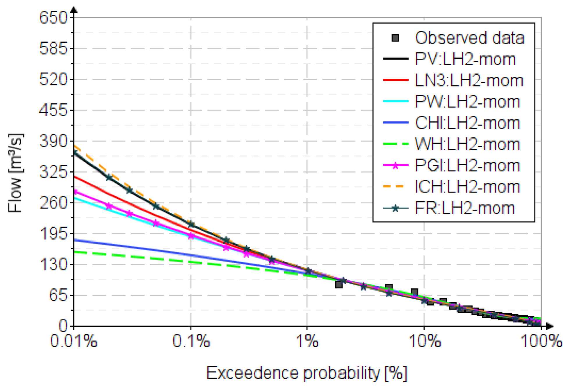
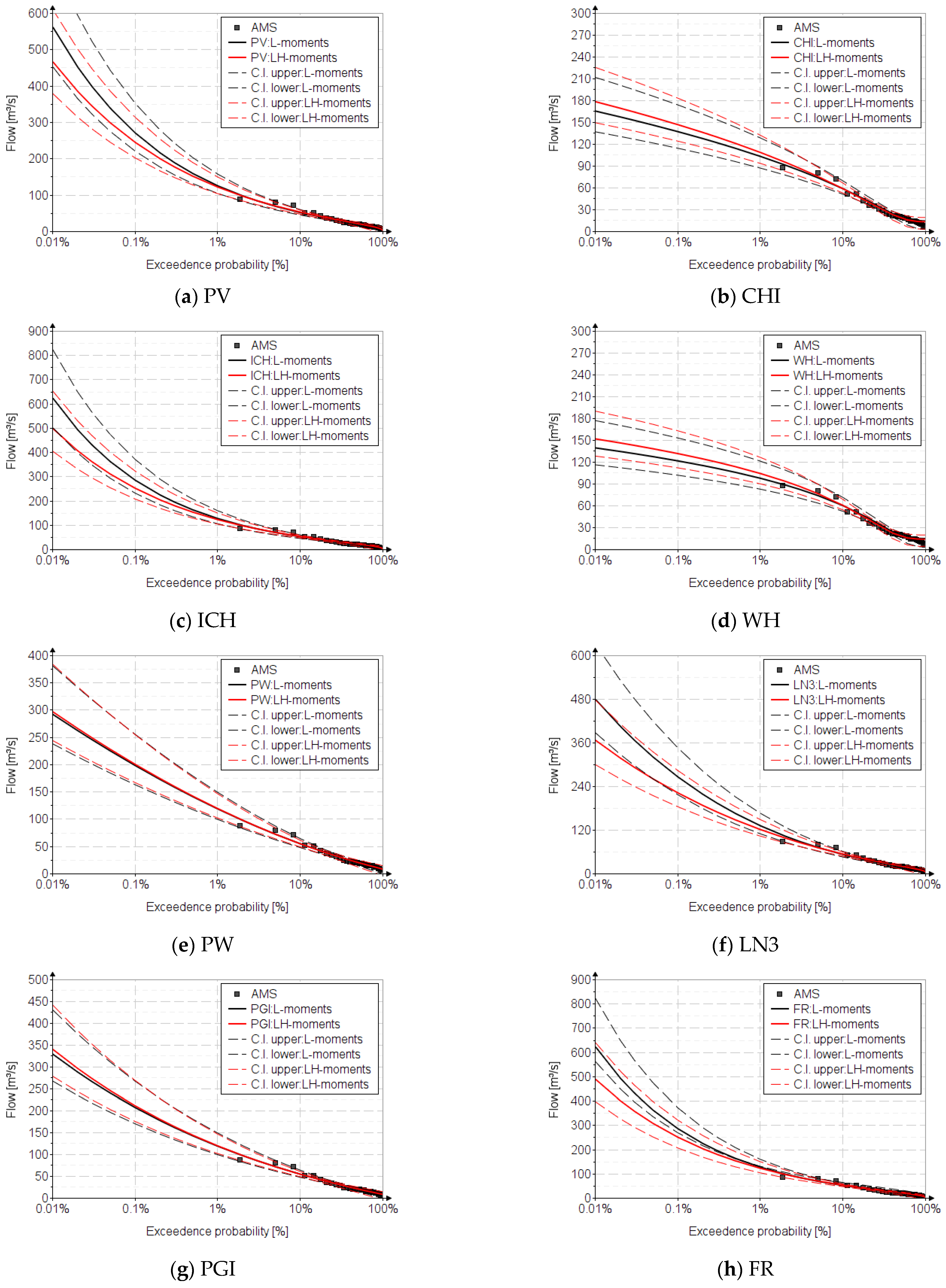
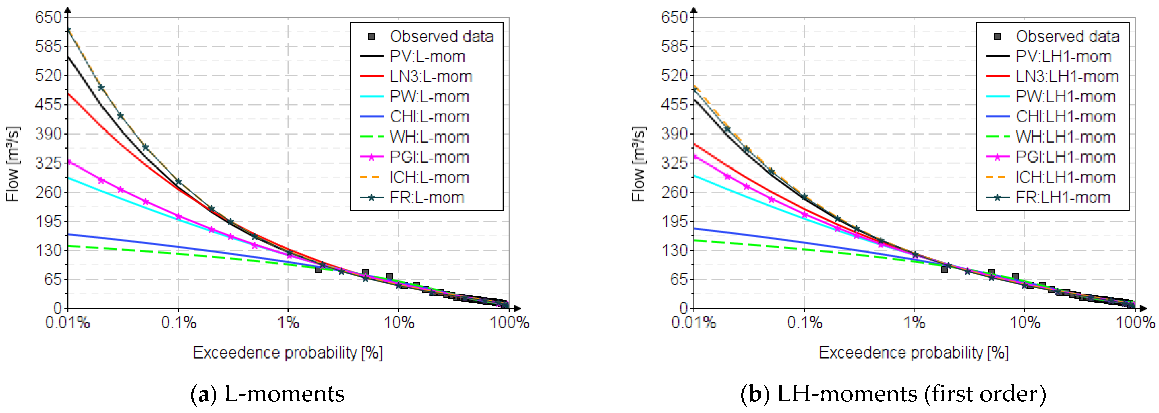
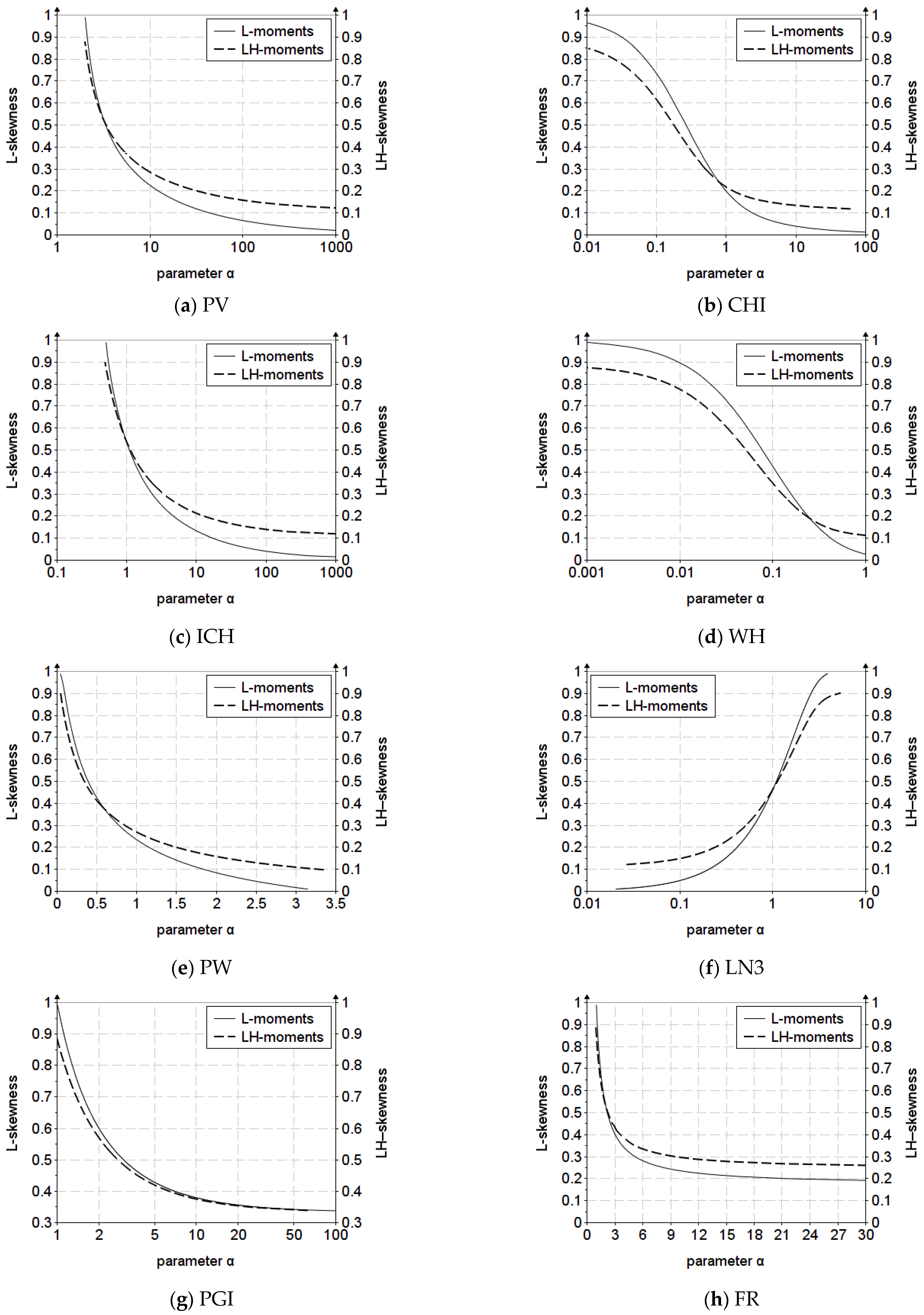
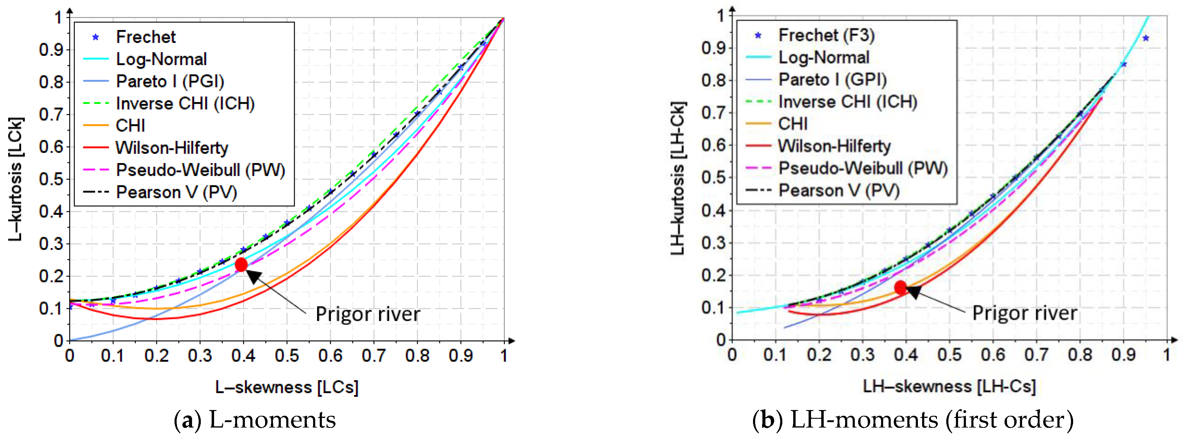
4. Results

In the flood frequency analysis, the most important quantiles are those for low exceeding probabilities because hydrotechnical constructions, especially dams, are designed based on these quantiles.

We present only the results obtained with the method of linear moments and the method of linear moments of first order, because these two methods are intended to be implemented in the future normative process of determining maximum flow rates in Romania. The distribution performance for second-order linear moments is presented in Appendix A.

Table 6 presents the quantiles for the most common exceedance probabilities in flood frequency analysis in the design of the dams.

Figure 3 shows the fitting distributions for the Prigor River. For plotting positions, the Alexeev formula was used [29].

In Figure A4 (Appendix J), the confidence interval for each analyzed distribution is presented for both methods using Chow’s relation for a 95% confidence level. Table 7 shows the values of the distribution parameters for the two methods of parameter estimation.

The performance of the analyzed distribution and the choice of the best-fit model were evaluated using the linear and higher-order linear moment values and diagrams.

The distribution performance values are presented in Table 8. The values for the best-fit model are highlighted in bold. The values of the RME and RAE indicators are presented informatively, knowing that they are relevant only in the area of the observed data.

5. Discussion

In flood frequency analysis, the main purpose is to determine, as accurately and rigorously as possible, the values of the quantiles that characterize the field of low exceedance probabilities, where generally there are no observed values.

As can be seen from the values in Table 6 and the graphics in Figure 3, the results characterizing the range of probabilities lower than 1% vary significantly, both between the analyzed distributions and between the estimation methods of the distribution parameters.

Regarding the results obtained for the same probability distributions but with different parameter estimation methods, for the CHI, WH, PW and PGI probability distributions, the values are not much different between the two methods. This is due to the variation in the shape parameter that characterizes the skewness, where the differences in its values are very small. It can also be observed in the variation graphs of the parameters of the analyzed distributions presented in Figure 4.

In the case of the PV, LN3, ICH and FR distributions, for the values of the statistical indicators L-skewness and LH-skewness of the analyzed observed data, the two values that characterize the shape parameter differ significantly between the two methods, an aspect highlighted by the obtained quantile values.

In the case of the Prigor River, among the distributions analyzed in this article, the Pseudo-Weibull, generalized Pareto Type I, CHI and Wilson–Hilferty distributions give the best results. The values of the natural indicators L-skewness and LH-skewness are the closest to the values of the corresponding indicators of the observed data, an aspect also highlighted in the graphs of Figure 5.

In the case of both parameter estimation methods, the application of a certain probability distribution of three parameters in the frequency analysis of extreme events in hydrology is carried out only if the theoretical values of the indicators L-skewness, L-kurtosis, LH-skewness and LH-kurtosis are closest to the corresponding values of the indicators of the analyzed data set, an aspect also highlighted in the literature [2,3,14,15,17,22,23]. The inconvenience of three-parameter distributions is due to the fact that they cannot calibrate higher-order linear moments (the fourth-order linear moment that characterizes L-kurtosis).

6. Conclusions

The LH-moments method has become one of the most commonly used methods for estimating statistical parameters without sample censoring in flood frequency analysis using the series of maximum annual flows.

This article presents all the necessary elements for the application of the eight probability distributions using the first and second LH methods.

The exact and approximate relations for estimating the distribution parameters are presented, as are exact and approximate relations for determining the frequency factor for a quick but accurate calculation of the most common occurring probabilities in flood frequency analysis (see Appendix E, Appendix F, Appendix G and Appendix H). In the case of the CHI, WH and PW distributions, the exact and approximate estimations of the frequency factor for the L-moments method were presented in previous research [20,21].

The variation graphs of the shape parameters for each distribution and each analyzed method are presented, as are the relative estimation errors of these parameters.

Considering that the main selection criterion in the case of these parameter estimation methods is represented by the values and the variation graphs of the statistical indicators, the variation relations for a wide range of distributions, including those analyzed in this article, are presented, providing information of real help in using these distributions.

In the case of the Prigor River, based on the selection criteria specific to these methods, among the presented distributions, the PW, GPI, CHI and WH distributions give the best results.

All this research is part of much more complex scientific research carried out within the Faculty of Hydrotechnics, in which a large number of distributions and families of distributions were analyzed using the method of ordinary moments and the method of linear moments, with results concretized in other papers [18,19,20,21,27,30].

The main purpose of this article is to present all the elements necessary for the application of these distributions in frequency analysis in hydrology using the LH-moments method and, in particular, the use of these distributions and methods in the elaboration of a normative regarding the determination of maximum flows in Romania, a normative that will contain dedicated, open-source applications with these elements.

Otherwise, these new elements will also be used for future regulations regarding the analysis of another extreme phenomenon in hydrology, namely water scarcity, which, in the context of climate change, becomes of particular importance (an aspect also highlighted in other publications [31,32]).

All the presented elements represent novelty elements and facilitate the ease of application of these probability distributions, which is important considering that the vast majority of the distributions used in frequency analysis in hydrology using the LH-moments method are not included in existing dedicated programs.

Author Contributions

Conceptualization, C.I. and C.G.A.; methodology, C.I. and C.G.A.; software, C.I. and C.G.A.; validation, C.I. and C.G.A.; formal analysis, C.I. and C.G.A.; investigation, C.I. and C.G.A.; resources, C.I. and C.G.A.; data curation, C.I. and C.G.A.; writing—original draft preparation, C.I. and C.G.A.; writing—review and editing, C.I. and C.G.A.; visualization, C.I. and C.G.A.; supervision, C.I. and C.G.A.; project administration, C.I. and C.G.A.; funding acquisition, C.I. and C.G.A. All authors have read and agreed to the published version of the manuscript.

Funding

This research received no external funding.

Data Availability Statement

Not applicable.

Conflicts of Interest

The authors declare no conflict of interest.

Abbreviations

MOM	the method of ordinary moments
L-moments	the method of linear moments
LH-moments	the method of higher-order linear moments
$L_{1}, L_{2}, L_{3}$	linear moments
$L_{H 1}, L_{H 2}, L_{H 3}$	higher-order linear moments
$τ_{2}, L C_{v}$	coefficient of variation based on the L-moments method
$τ_{3}, L C_{s}$	coefficient of skewness based on the L-moments method
$τ_{4}, L C_{k}$	coefficient of kurtosis based on the L-moments method
$τ_{H 2}, L H - C_{v}$	coefficient of variation based on the LH-moments method
$τ_{H 3}, L H - C_{s}$	coefficient of skewness based on the LH-moments method
$τ_{H 4}, L H - C_{k}$	coefficient of kurtosis based on the LH-moments method
PV	Pearson V distribution
CHI	CHI distribution
ICH	inverse CHI distribution
WH	Wilson–Hilferty distribution
PW	Pseudo-Weibull distribution
LN3	three-parameter Log-normal distribution
GPI	generalized Pareto Type I distribution
FR	three-parameter Fréchet distribution

Appendix A. Parameter Estimation Using the Second-Order LH-Moments

The statistical indicators are calculated using the specific relations of the second-order LH method [1].

Pearson V (PV) distribution

The shape parameter

α

can be evaluated numerically with the following approximate forms, depending on LH-skewness (

0.2 < |τ_{H 3}| \leq 0.8

):

α = \exp (\begin{array}{l} 0 . 7703254 + 1 . 8023535 \cdot \ln (|τ_{H 3}|) + 12 . 0654748 \cdot \ln {(|τ_{H 3}|)}^{2} + \\ 31 . 3070953 \cdot \ln {(|τ_{H 3}|)}^{3} + 50 . 0185737 \cdot \ln {(|τ_{H 3}|)}^{4} + 48 . 0218148 \cdot \ln {(|τ_{H 3}|)}^{5} + \\ 27 . 8335549 \cdot \ln {(|τ_{H 3}|)}^{6} + 8 . 9904377 \cdot \ln {(|τ_{H 3}|)}^{7} + 1 . 2597532 \cdot \ln {(|τ_{H 3}|)}^{8} \end{array})

The scale parameter

β

and the position parameter

γ

are determined by the following expressions:

β = \frac{L_{H 2}}{z_{1}}

γ = L_{H 1} - 3 \cdot β \cdot z_{2}

where

z_{1} = \int_{0}^{1} \frac{1}{q g a m m a (1 - p, α - 1)} \cdot (8 \cdot p^{3} - 6 \cdot p^{2}) \cdot d p

, which can be approximated with the following equation:

z_{1} = \exp (\begin{array}{l} 70 . 068220301 - 253 . 066147842 \cdot \ln (α) + 405 . 371887371 \cdot \ln {(α)}^{2} - \\ 375 . 469158123 \cdot \ln {(α)}^{3} + 218 . 079975625 \cdot \ln {(α)}^{4} - 82 . 183290073 \cdot \ln {(α)}^{5} + \\ 20 . 100915955 \cdot \ln {(α)}^{6} - 3 . 080861051 \cdot \ln {(α)}^{7} + 0 . 268939488 \cdot \ln {(α)}^{8} - 0 . 010204593 \cdot \ln {(α)}^{9} \end{array})

and

z_{2} = \int_{0}^{1} \frac{1}{q g a m m a (1 - p, α - 1)} \cdot p^{2} \cdot d p

, which can be approximated with the following equation:

z_{2} = \exp (\begin{array}{l} 65 . 5870555 - 241 . 6468173 \cdot \ln (α) + 391 . 1225404 \cdot \ln {(α)}^{2} - \\ 363 . 9624699 \cdot \ln {(α)}^{3} + 212 . 019458 \cdot \ln {(α)}^{4} - 80 . 064287 \cdot \ln {(α)}^{5} + \\ 19 . 6131341 \cdot \ln {(α)}^{6} - 3 . 0098374 \cdot \ln {(α)}^{7} + 0 . 2630127 \cdot \ln {(α)}^{8} - 0 . 0099887 \cdot \ln {(α)}^{9} \end{array})

Pseudo-Weibull (PW) distribution

The shape parameter

α

can be evaluated numerically with the following approximate forms, depending on LH-skewness (

0.2 < |τ_{H 3}| \leq 0.8

):

α = \exp (\begin{array}{l} - 5 . 2225077 - 17 . 8654702 \cdot \ln (|τ_{H 3}|) - 43 . 4458049 \cdot \ln {(|τ_{H 3}|)}^{2} - \\ 69 . 6462537 \cdot \ln {(|τ_{H 3}|)}^{3} - 68 . 8374609 \cdot \ln {(|τ_{H 3}|)}^{4} - 42 . 2639586 \cdot \ln {(|τ_{H 3}|)}^{5} - \\ 15 . 7018547 \cdot \ln {(|τ_{H 3}|)}^{6} - 3 . 2319781 \cdot \ln {(|τ_{H 3}|)}^{7} - 0 . 2826753 \cdot \ln {(|τ_{H 3}|)}^{8} \end{array})

The scale parameter

β

and the position parameter

γ

are determined by the following expressions:

β = \frac{L_{H 2}}{z_{1}}

γ = L_{H 1} - 3 \cdot β \cdot z_{2}

where

z_{1} = \int_{0}^{1} q g a m m a {(p, \frac{1}{α} + 1)}^{\frac{1}{α}} \cdot (8 \cdot p^{3} - 6 \cdot p^{2}) \cdot d p

, which can be approximated with the following equation:

z_{1} = \exp (\begin{array}{l} - 0 . 40607485 - 2 . 368325995 \cdot \ln (α) + 1 . 154932857 \cdot \ln {(α)}^{2} - \\ 0 . 51477681 \cdot \ln {(α)}^{3} + 0 . 154969653 \cdot \ln {(α)}^{4} - 0 . 058279056 \cdot \ln {(α)}^{5} + 0 . 014783487 \cdot \ln {(α)}^{6} \end{array})

and

z_{2} = \int_{0}^{1} q g a m m a {(p, \frac{1}{α} + 1)}^{\frac{1}{α}} \cdot p^{2} \cdot d p

, which can be approximated with the following equation:

z_{2} = \exp (\begin{array}{l} 0 . 0671983 - 1 . 6755793 \cdot \ln (α) + 1 . 213393 \cdot \ln {(α)}^{2} - \\ 0 . 5661667 \cdot \ln {(α)}^{3} + 0 . 1746241 \cdot \ln {(α)}^{4} - 0 . 0389579 \cdot \ln {(α)}^{5} + \\ 0 . 0109139 \cdot \ln {(α)}^{6} - 0 . 0024496 \cdot \ln {(α)}^{7} \end{array})

Fréchet (FR) distribution

The equations needed to estimate the parameters with LH-moments have the following expressions:

L_{H 1} = γ + β \cdot 3^{\frac{1}{α}} \cdot Γ (1 - \frac{1}{α})

L_{H 2} = \frac{β \cdot π \cdot (2^{\frac{2}{α} + 1} - 2 \cdot 3^{\frac{1}{α}})}{Γ (\frac{1}{α}) \cdot \sin (\frac{π}{α})}

L_{H 3} = \frac{β \cdot 5 \cdot π \cdot (6 \cdot 5^{\frac{1}{α}} + 2 \cdot 3^{\frac{1}{α}} - 5 \cdot 4^{\frac{1}{α}})}{3 \cdot Γ (\frac{1}{α}) \cdot \sin (\frac{π}{α})}

The parameter

α

can be approximated using the next relation, depending on

τ_{H 3}

:

if $0.28 < |τ_{H 3}| \leq 0.45$ :

α = \exp (\begin{array}{l} - 749480 . 96282 - 6708919 . 18032 \cdot \ln (|τ_{H 3}|) - 26612862 . 7257 \cdot \ln {(|τ_{H 3}|)}^{2} - \\ 61402618 . 18226 \cdot \ln {(|τ_{H 3}|)}^{3} - 90812958 . 2641 \cdot \ln {(|τ_{H 3}|)}^{4} - \\ 89285821 . 56955 \cdot \ln {(|τ_{H 3}|)}^{5} - 58358858 . 11388 \cdot \ln {(|τ_{H 3}|)}^{6} - \\ 24453687 . 54297 \cdot \ln {(|τ_{H 3}|)}^{7} - 5960979 . 27152 \cdot \ln {(|τ_{H 3}|)}^{8} - 644094 . 53004 \cdot \ln {(|τ_{H 3}|)}^{9} \end{array})

if $0.45 < |τ_{H 3}| \leq 0.90$ :

α = \exp (\begin{array}{l} - 0 . 2236259 - 1 . 1243974 \cdot \ln (|τ_{H 3}|) + 0 . 6247787 \cdot \ln {(|τ_{H 3}|)}^{2} + \\ 0 . 493862 \cdot \ln {(|τ_{H 3}|)}^{3} + 0 . 6072315 \cdot \ln {(|τ_{H 3}|)}^{4} \end{array})

The scale parameter

β

and the position parameter

γ

are determined by the following expressions:

β = \frac{L_{H 2} \cdot Γ (\frac{1}{α}) \cdot \sin (\frac{π}{α})}{π \cdot (2^{\frac{2}{α} + 1} - 2 \cdot 3^{\frac{1}{α}})}

γ = L_{H 1} - β \cdot 3^{\frac{1}{α}} \cdot Γ (1 - \frac{1}{α})

Wilson–Hilferty (WH) distribution

The shape parameter

α

can be evaluated numerically with the following approximate forms, depending on LH-skewness (

0.16 < |τ_{H 3}| \leq 0.8

):

α = \exp (\begin{array}{l} - 24 . 2717598 - 199 . 9827559 \cdot \ln (|τ_{H 3}|) - 907 . 1696354 \cdot \ln {(|τ_{H 3}|)}^{2} - \\ 2393 . 7758375 \cdot \ln {(|τ_{H 3}|)}^{3} - 3946 . 6821282 \cdot \ln {(|τ_{H 3}|)}^{4} - 4196 . 8735478 \cdot \ln {(|τ_{H 3}|)}^{5} - \\ 2878 . 4415831 \cdot \ln {(|τ_{H 3}|)}^{6} - 1229 . 852233 \cdot \ln {(|τ_{H 3}|)}^{7} - 297 . 7079385 \cdot \ln {(|τ_{H 3}|)}^{8} - \\ 31 . 1843533 \cdot \ln {(|τ_{H 3}|)}^{9} \end{array})

The scale parameter

β

and the position parameter

γ

are determined by the following expressions:

β = \frac{L_{H 2}}{z_{1}}

γ = L_{H 1} - 3 \cdot β \cdot z_{2}

where

z_{1} = \int_{0}^{1} q g a m m a {(p, α)}^{\frac{1}{3}} \cdot (8 \cdot p^{3} - 6 \cdot p^{2}) \cdot d p

, which can be approximated with the following equation:

z_{1} = \exp (\begin{array}{l} - 2 . 085292134 - 0 . 150846234 \cdot \ln (α) + 0 . 012279379 \cdot \ln {(α)}^{2} - \\ 0 . 011892699 \cdot \ln {(α)}^{3} - 0 . 021740029 \cdot \ln {(α)}^{4} - \\ 0 . 004444376 \cdot \ln {(α)}^{5} - 0 . 000269647 \cdot \ln {(α)}^{6} \end{array})

and

z_{2} = \int_{0}^{1} q g a m m a {(p, α)}^{\frac{1}{3}} \cdot p^{2} \cdot d p

, which can be approximated with the following equation:

z_{2} = \exp (\begin{array}{l} - 0 . 9433178 + 0 . 2891917 \cdot \ln (α) - 0 . 0525735 \cdot \ln {(α)}^{2} - \\ 0 . 0287951 \cdot \ln {(α)}^{3} - 0 . 0231076 \cdot \ln {(α)}^{4} - \\ 0 . 0060035 \cdot \ln {(α)}^{5} - 0 . 0006706 \cdot \ln {(α)}^{6} - 0 . 0000281 \cdot \ln {(α)}^{7} \end{array})

Log-Normal (LN3) distribution

The scale parameter

β

can be evaluated numerically with the following approximate forms, depending on LH-skewness (

0.16 < τ_{H 3} \leq 0.8

):

β = \exp (\begin{array}{l} 5 . 5997658 + 53 . 4446795 \cdot \ln (|τ_{H 3}|) + 280 . 5758463 \cdot \ln {(|τ_{H 3}|)}^{2} + \\ 866 . 7797953 \cdot \ln {(|τ_{H 3}|)}^{3} + 1659 . 7530346 \cdot \ln {(|τ_{H 3}|)}^{4} + 2033 . 1857675 \cdot \ln {(|τ_{H 3}|)}^{5} + \\ 1592 . 7716345 \cdot \ln {(|τ_{H 3}|)}^{6} + 770 . 8810928 \cdot \ln {(|τ_{H 3}|)}^{7} + 209 . 7251296 \cdot \ln {(|τ_{H 3}|)}^{8} + \\ 24 . 5139669 \cdot \ln {(|τ_{H 3}|)}^{9} \end{array})

The shape parameter

α

and the position parameter

γ

are determined by the following expressions:

α = \ln (\frac{L_{H 2}}{z_{1}})

γ = L_{H 1} - 3 \cdot \exp (α) \cdot z_{2}

where

z_{1} = \int_{0}^{1} \exp (β \cdot q n o r m (p, 0, 1)) \cdot (8 \cdot p^{3} - 6 \cdot p^{2}) \cdot d p

, which can be approximated with the following equation:

z_{1} = \exp (\begin{array}{l} 0 . 014722846 + 2 . 299838276 \cdot \ln (β) + 0 . 925071272 \cdot \ln {(β)}^{2} + \\ 0 . 526679239 \cdot \ln {(β)}^{3} + 0 . 297100461 \cdot \ln {(β)}^{4} + 0 . 142726563 \cdot \ln {(β)}^{5} + \\ 0 . 043986648 \cdot \ln {(β)}^{6} + 0 . 007187861 \cdot \ln {(β)}^{7} + 0 . 000469736 \cdot \ln {(β)}^{8} \end{array})

and

z_{2} = \int_{0}^{1} \exp (β \cdot q n o r m (p, 0, 1)) \cdot p^{2} \cdot d p

, which can be approximated with the following equation:

z_{2} = \exp (\begin{array}{l} 0 . 0441496 + 1 . 4591307 \cdot \ln (β) + 1 . 0576843 \cdot \ln {(β)}^{2} + \\ 0 . 5860892 \cdot \ln {(β)}^{3} + 0 . 292079 \cdot \ln {(β)}^{4} + 0 . 1379002 \cdot \ln {(β)}^{5} + \\ 0 . 0524525 \cdot \ln {(β)}^{6} + 0 . 0130832 \cdot \ln {(β)}^{7} + 0 . 0018047 \cdot \ln {(β)}^{8} + 0 . 0001031 \cdot \ln {(β)}^{9} \end{array})

CHI distribution

The shape parameter

α

can be evaluated numerically with the following approximate forms, depending on LH-skewness (

0.2 < |τ_{H 3}| \leq 0.8

):

α = \exp (\begin{array}{l} - 25 . 6337507 - 236 . 6618708 \cdot \ln (|τ_{H 3}|) - 1126 . 3329329 \cdot \ln {(|τ_{H 3}|)}^{2} - \\ 3104 . 9770673 \cdot \ln {(|τ_{H 3}|)}^{3} - 5335 . 3285993 \cdot \ln {(|τ_{H 3}|)}^{4} - \\ 5903 . 6543563 \cdot \ln {(|τ_{H 3}|)}^{5} - 4209 . 4097095 \cdot \ln {(|τ_{H 3}|)}^{6} - \\ 1869 . 4841235 \cdot \ln {(|τ_{H 3}|)}^{7} - 470 . 7309743 \cdot \ln {(|τ_{H 3}|)}^{8} - 51 . 3805751 \cdot \ln {(|τ_{H 3}|)}^{9} \end{array})

The scale parameter

β

and the position parameter

γ

are determined by the following expressions:

β = \frac{L_{H 2}}{z_{1}}

γ = L_{H 1} - 3 \cdot β \cdot z_{2}

where

z_{1} = \int_{0}^{1} \sqrt{2 \cdot q g a m m a (p, \frac{α}{2})} \cdot (8 \cdot p^{3} - 6 \cdot p^{2}) \cdot d p

, which can be approximated with the following equation:

z_{1} = \exp (\begin{array}{l} - 1 . 282810649 + 0 . 027979479 \cdot \ln (α) - 0 . 05033417 \cdot \ln {(α)}^{2} + \\ 0 . 021850999 \cdot \ln {(α)}^{3} - 0 . 001932334 \cdot \ln {(α)}^{4} - \\ 0 . 000810088 \cdot \ln {(α)}^{5} + 0 . 000082461 \cdot \ln {(α)}^{6} + 0 . 000016615 \cdot \ln {(α)}^{7} \end{array})

and

z_{2} = \int_{0}^{1} \sqrt{2 \cdot q g a m m a (p, \frac{α}{2})} \cdot p^{2} \cdot d p

, which can be approximated with the following equation:

z_{2} = \exp (\begin{array}{l} - 0 . 8159636 + 0 . 484355 \cdot \ln (α) - 0 . 0434581 \cdot \ln {(α)}^{2} + \\ 0 . 013379 \cdot \ln {(α)}^{3} + 0 . 0001081 \cdot \ln {(α)}^{4} - 0 . 0005661 \cdot \ln {(α)}^{5} + \\ 0 . 0000168 \cdot \ln {(α)}^{6} + 0 . 0000115 \cdot \ln {(α)}^{7} \end{array})

Inverse CHI (ICH) distribution

The shape parameter

α

can be evaluated numerically with the following approximate forms, depending on LH-skewness (

0.2 < |τ_{H 3}| \leq 0.8

):

α = \exp (\begin{array}{l} - 1 . 1409838 - 3 . 7281901 \cdot \ln (|τ_{H 3}|) - 11 . 4041535 \cdot \ln {(|τ_{H 3}|)}^{2} - \\ 28 . 1895148 \cdot \ln {(|τ_{H 3}|)}^{3} - 37 . 6078101 \cdot \ln {(|τ_{H 3}|)}^{4} - 28 . 8259956 \cdot \ln {(|τ_{H 3}|)}^{5} - \\ 11 . 7387827 \cdot \ln {(|τ_{H 3}|)}^{6} - 2 . 0006845 \cdot \ln {(|τ_{H 3}|)}^{7} \end{array})

The scale parameter

β

and the position parameter

γ

are determined by the following expressions:

β = \frac{L_{H 2}}{z_{1}}

γ = L_{H 1} - 3 \cdot β \cdot z_{2}

where

z_{1} = \int_{0}^{1} \frac{1}{\sqrt{q g a m m a (1 - p, α)}} \cdot (8 \cdot p^{3} - 6 \cdot p^{2}) \cdot d p

, which can be approximated with the following equation:

z_{1} = \exp (\begin{array}{l} - 0 . 057334428 - 2 . 622136121 \cdot \ln (α) + 1 . 262885759 \cdot \ln {(α)}^{2} - \\ 2 . 0026002 \cdot \ln {(α)}^{3} + 2 . 983910396 \cdot \ln {(α)}^{4} - \\ 2 . 546891691 \cdot \ln {(α)}^{5} + 1 . 233970727 \cdot \ln {(α)}^{6} - \\ 0 . 340022204 \cdot \ln {(α)}^{7} + 0 . 049778844 \cdot \ln {(α)}^{8} - 0 . 003009371 \cdot \ln {(α)}^{9} \end{array})

and

z_{2} = \int_{0}^{1} \frac{1}{\sqrt{q g a m m a (1 - p, α)}} \cdot p^{2} \cdot d p

, which can be approximated with the following equation:

z_{2} = \exp (\begin{array}{l} 0 . 016945843 - 1 . 719328787 \cdot \ln (α) + 1 . 152177296 \cdot \ln {(α)}^{2} - \\ 1 . 836394903 \cdot \ln {(α)}^{3} + 2 . 539946588 \cdot \ln {(α)}^{4} - \\ 2 . 07825526 \cdot \ln {(α)}^{5} + 0 . 983614297 \cdot \ln {(α)}^{6} - \\ 0 . 267138228 \cdot \ln {(α)}^{7} + 0 . 038725467 \cdot \ln {(α)}^{8} - 0 . 002324394 \cdot \ln {(α)}^{9} \end{array})

Generalized Pareto Type I (PGI)

The equations needed to estimate the parameters with LH-moments have the following expressions:

L_{H 1} = γ + β \cdot (\frac{11 \cdot α^{2} - 6 \cdot α + 1}{(α - 1) \cdot (2 \cdot α - 1) \cdot (3 \cdot α - 1)} + 1)

L_{H 2} = \frac{12 \cdot α^{3} \cdot β}{(α - 1) \cdot (2 \cdot α - 1) \cdot (3 \cdot α - 1) \cdot (4 \cdot α - 1)}

L_{H 3} = \frac{20 \cdot α^{3} \cdot β \cdot (α + 1)}{(α - 1) \cdot (2 \cdot α - 1) \cdot (3 \cdot α - 1) \cdot (4 \cdot α - 1) \cdot (5 \cdot α - 1)}

The parameters have the following expressions:

α = \frac{3 \cdot τ_{H 3} + 5}{15 \cdot τ_{H 3} - 5}

β = \frac{L_{H 2} \cdot (α - 1) \cdot (2 \cdot α - 1) \cdot (3 \cdot α - 1) \cdot (4 \cdot α - 1)}{12 \cdot α^{3}}

λ = L_{H 1} - β \cdot (\frac{11 \cdot α^{2} - 6 \cdot α + 1}{(α - 1) \cdot (2 \cdot α - 1) \cdot (3 \cdot α - 1)} + 1)

Figure A1 shows the fitting distributions for the Prigor River for the second-order LH-moments.

Figure A1. Evaluation of the quantile function for the second-order LH-moments.

Appendix B. The Frequency Factors for the Analyzed Distributions

Table A1 shows the expressions of the frequency factors for the L-moments and LH-moments methods.

Table A1. Frequency factors.

Distr.	$Frequency Factor K_{p} (p)$
	Quantile Function (Inverse Function)
	LH-Moments (First Order)	LH-Moments (Second Order)
	$x (p) = L_{H 1} + L_{H 2} \cdot K_{p} (p)$
PV	$\frac{\frac{1}{q g a m m a (p, α - 1)} - 2 \cdot z_{2}}{\frac{3}{2} \cdot z_{1}}$ the expressions for $z_{1}$ and $z_{2}$ are explained in Section 2.2.1	$\frac{\frac{1}{q g a m m a (p, α - 1)} - 3 \cdot z_{2}}{z_{1}}$ the expressions for $z_{1}$ and $z_{2}$ are explained in Appendix A
CHI	$\frac{\sqrt{2 \cdot q g a m m a (1 - p, \frac{α}{2})} - 2 \cdot z_{2}}{\frac{3}{2} \cdot z_{1}}$ the expressions for $z_{1}$ and $z_{2}$ are explained in Section 2.2.4	$\frac{\sqrt{2 \cdot q g a m m a (1 - p, \frac{α}{2})} - 3 \cdot z_{2}}{z_{1}}$ the expressions for $z_{1}$ and $z_{2}$ are explained in Appendix A
ICH	$\frac{\frac{1}{\sqrt{q g a m m a (p, α)}} - 2 \cdot z_{2}}{\frac{3}{2} \cdot z_{1}}$ the expressions for $z_{1}$ and $z_{2}$ are explained in Section 2.2.3	$\frac{\frac{1}{\sqrt{q g a m m a (p, α)}} - 3 \cdot z_{2}}{z_{1}}$ the expressions for $z_{1}$ and $z_{2}$ are explained in Appendix A
WH	$\frac{q g a m m a {(1 - p, α)}^{\frac{1}{3}} - 2 \cdot z_{2}}{\frac{3}{2} \cdot z_{1}}$ the expressions for $z_{1}$ and $z_{2}$ are explained in Section 2.2.4	$\frac{q g a m m a {(1 - p, α)}^{\frac{1}{3}} - 3 \cdot z_{2}}{z_{1}}$ the expressions for $z_{1}$ and $z_{2}$ are explained in Appendix A
PW	$\frac{q g a m m a {(1 - p, \frac{1}{α} + 1)}^{\frac{1}{α}} - 2 \cdot z_{2}}{\frac{3}{2} \cdot z_{1}}$ the expressions for $z_{1}$ and $z_{2}$ are explained in Section 2.2.5	$\frac{q g a m m a {(1 - p, \frac{1}{α} + 1)}^{\frac{1}{α}} - 3 \cdot z_{2}}{z_{1}}$ the expressions for $z_{1}$ and $z_{2}$ are explained in Appendix A
LN3	$\frac{\exp (β \cdot q n o r m (1 - p, 0, 1)) - 2 \cdot z_{2}}{\frac{3}{2} \cdot z_{1}}$ the expressions for $z_{1}$ and $z_{2}$ are explained in Section 2.2.6	$\frac{\exp (β \cdot q n o r m (1 - p, 0, 1)) - 3 \cdot z_{2}}{z_{1}}$ the expressions for $z_{1}$ and $z_{2}$ are explained in Appendix A
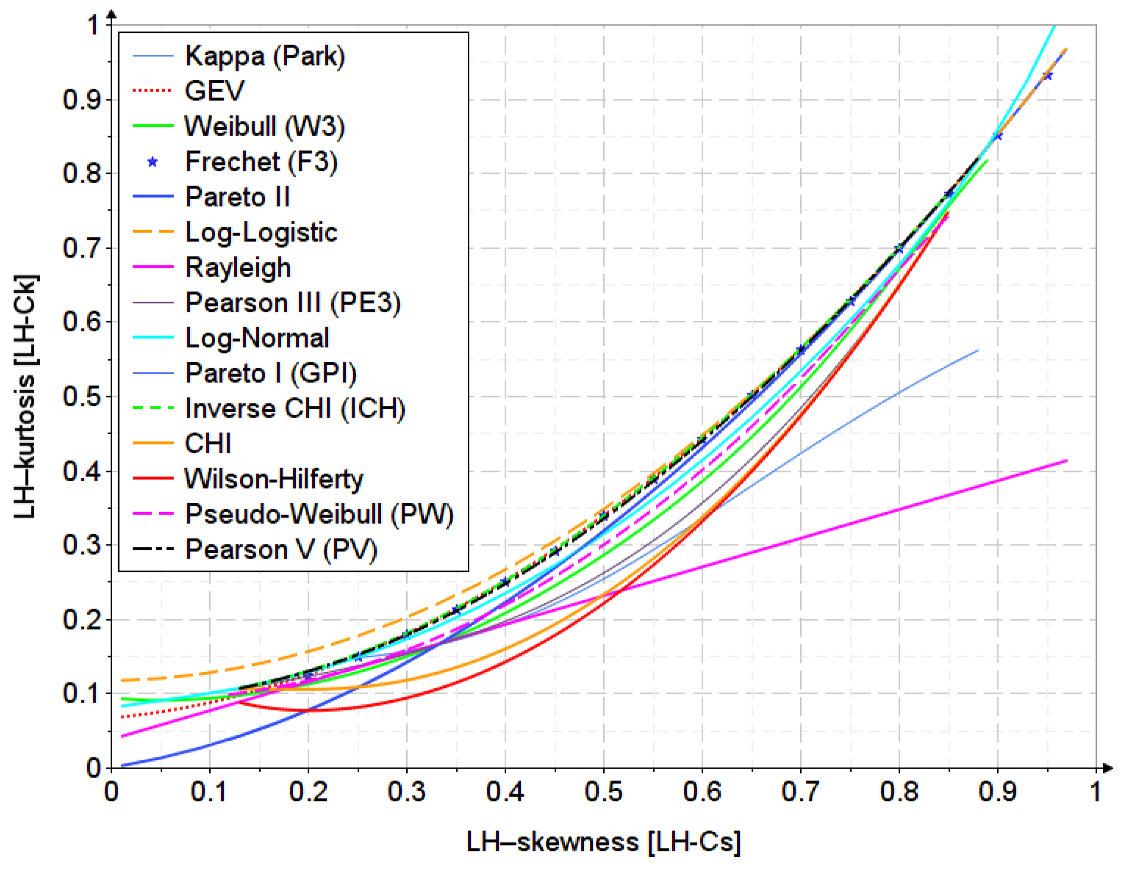
PGI	$\frac{(3 \cdot α - 1) (p^{- \frac{1}{α}} \cdot (2 \cdot α^{2} - 3 \cdot α + 1) - 2 \cdot α^{2})}{3 \cdot α^{2}}$	$\frac{(4 \cdot α - 1) (p^{- \frac{1}{α}} \cdot (6 \cdot α^{3} - 11 \cdot α^{2} + 6 \cdot α - 1) - 6 \cdot α^{3})}{12 \cdot α^{3}}$
FR	$\frac{2 \cdot Γ (\frac{1}{α}) \cdot \sin (\frac{π}{α}) \cdot {(- \ln (1 - p))}^{- \frac{1}{α}} - π \cdot 2^{\frac{1}{α} + 1}}{π \cdot (3^{\frac{1}{α} + 1} - 3 \cdot 2^{\frac{1}{α}})}$	$\frac{π \cdot 3^{\frac{1}{α}} - Γ (\frac{1}{α}) \cdot \sin (\frac{π}{α}) \cdot {(- \ln (1 - p))}^{- \frac{1}{α}}}{2 \cdot π \cdot (3^{\frac{1}{α}} - 2^{\frac{2}{α}})}$

Appendix C. The First-Order LH-Moments Diagram

In the next section, the variation in the first-order LH-kurtosis depending on the positive first-order LH-skewness is presented for certain theoretical distributions often used in hydrology and in this article.

Figure A2. The variation diagram for the first-order LH-skewness and LH-kurtosis.

Pearson III:

\begin{array}{l} τ_{H 4} = 0 . 1012322 - 0 . 2437927 \cdot τ_{H 3} + 3 . 5538482 \cdot τ_{H 3}^{2} - 13 . 8996553 \cdot τ_{H 3}^{3} + 31 . 3422272 \cdot τ_{H 3}^{4} - \\ 35 . 5781144 \cdot τ_{H 3}^{5} + 20 . 677076 \cdot τ_{H 3}^{6} - 4 . 8315272 \cdot τ_{H 3}^{7} \end{array}

Log-normal:

\begin{array}{l} τ_{H 4} = 0 . 0801496 + 0 . 2283728 \cdot τ_{H 3} - 0 . 9987353 \cdot τ_{H 3}^{2} + 8 . 8369201 \cdot τ_{H 3}^{3} - 24 . 2488462 \cdot τ_{H 3}^{4} + \\ 37 . 7635295 \cdot τ_{H 3}^{5} - 30 . 6596349 \cdot τ_{H 3}^{6} + 10 . 1236239 \cdot τ_{H 3}^{7} \end{array}

GEV:

\begin{array}{l} τ_{H 4} = 0 . 066585 + 0 . 1207821 \cdot τ_{H 3} + 0 . 8711194 \cdot τ_{H 3}^{2} - 0 . 0456666 \cdot τ_{H 3}^{3} - 0 . 0033066 \cdot τ_{H 3}^{4} + \\ 0 . 0170713 \cdot τ_{H 3}^{5} - 0 . 0094267 \cdot τ_{H 3}^{6} + 0 . 0009899 \cdot τ_{H 3}^{7} \end{array}

Weibull:

\begin{array}{l} τ_{H 4} = 0 . 0940624 - 0 . 167248 \cdot τ_{H 3} + 2 . 2686976 \cdot τ_{H 3}^{2} - 9 . 8557774 \cdot τ_{H 3}^{3} + 35 . 7330334 \cdot τ_{H 3}^{4} - \\ 66 . 7529615 \cdot τ_{H 3}^{5} + 61 . 9426076 \cdot τ_{H 3}^{6} - 22 . 3935866 \cdot τ_{H 3}^{7} \end{array}

Rayleigh:

τ_{H 4} = \frac{7 \cdot (\sqrt{10} + 4 - 5 \cdot \sqrt{2}) \cdot (3 \cdot τ_{H 3} - 1)}{30 \cdot \sqrt{6} - 10 \cdot \sqrt{2} - 60} + \frac{99 \cdot τ_{H 3} - 28}{30}

Log-logistic:

τ_{H 4} = \frac{170 \cdot τ_{H 3}^{2} + 36 \cdot τ_{H 3} + 224}{1920}

Fréchet:

\begin{array}{l} τ_{H 4} = 0 . 0022429 + 0 . 9647477 \cdot τ_{H 3} - 3 . 6860338 \cdot τ_{H 3}^{2} + 13 . 1297753 \cdot τ_{H 3}^{3} - 22 . 1386065 \cdot τ_{H 3}^{4} + \\ 21 . 7301791 \cdot τ_{H 3}^{5} - 11 . 5710264 \cdot τ_{H 3}^{6} + 2 . 5873135 \cdot τ_{H 3}^{7} \end{array}

Kappa (generalized Gumbel, Jeong 2009):

\begin{array}{l} τ_{H 4} = 0 . 2623693 - 1 . 8726094 \cdot τ_{H 3} + 12 . 2859097 \cdot τ_{H 3}^{2} - 45 . 0169093 \cdot τ_{H 3}^{3} + 100 . 4606818 \cdot τ_{H 3}^{4} - \\ 122 . 9124059 \cdot τ_{H 3}^{5} + 76 . 5421309 \cdot τ_{H 3}^{6} - 19 . 1260088 \cdot τ_{H 3}^{7} \end{array}

Pearson V:

\begin{array}{l} τ_{H 4} = 0 . 0698137 + 0 . 3768677 \cdot τ_{H 3} - 1 . 8015231 \cdot τ_{H 3}^{2} + 10 . 5928008 \cdot τ_{H 3}^{3} - 22 . 5459968 \cdot τ_{H 3}^{4} + \\ 27 . 1756708 \cdot τ_{H 3}^{5} - 17 . 5457 \cdot τ_{H 3}^{6} + 4 . 7032094 \cdot τ_{H 3}^{7} \end{array}

Pseudo-Weibull:

\begin{array}{l} τ_{H 4} = 0 . 1247692 - 0 . 8132588 \cdot τ_{H 3} + 7 . 8245742 \cdot τ_{H 3}^{2} - 32 . 9812148 \cdot τ_{H 3}^{3} + 89 . 3432014 \cdot τ_{H 3}^{4} - \\ 136 . 9045781 \cdot τ_{H 3}^{5} + 110 . 4775227 \cdot τ_{H 3}^{6} - 36 . 3378089 \cdot τ_{H 3}^{7} \end{array}

Wilson–Hilferty:

\begin{array}{l} τ_{H 4} = 0 . 1963258 - 1 . 5474914 \cdot τ_{H 3} + 7 . 4777715 \cdot τ_{H 3}^{2} - 19 . 8099209 \cdot τ_{H 3}^{3} + 38 . 3808311 \cdot τ_{H 3}^{4} - \\ 43 . 3828583 \cdot τ_{H 3}^{5} + 26 . 5600641 \cdot τ_{H 3}^{6} - 6 . 7790242 \cdot τ_{H 3}^{7} \end{array}

CHI:

\begin{array}{l} τ_{H 4} = 0 . 0469014 + 1 . 2890443 \cdot τ_{H 3} - 10 . 3957874 \cdot τ_{H 3}^{2} + 38 . 4367035 \cdot τ_{H 3}^{3} - 69 . 8260621 \cdot τ_{H 3}^{4} + \\ 70 . 9754662 \cdot τ_{H 3}^{5} - 36 . 8705108 \cdot τ_{H 3}^{6} + 7 . 4087633 \cdot τ_{H 3}^{7} \end{array}

Inverse CHI:

\begin{array}{l} τ_{H 4} = 0 . 0892257 + 0 . 0403381 \cdot τ_{H 3} + 0 . 4733583 \cdot τ_{H 3}^{2} + 2 . 80145 \cdot τ_{H 3}^{3} - 6 . 8676052 \cdot τ_{H 3}^{4} + \\ 8 . 32418 \cdot τ_{H 3}^{5} - 5 . 0845891 \cdot τ_{H 3}^{6} + 1 . 2372547 \cdot τ_{H 3}^{7} \end{array}

Generalized Pareto Type I:

τ_{H 4} = \frac{45 \cdot τ_{H 3} - 350}{6} + \frac{1400}{3 \cdot τ_{H 3} + 24}

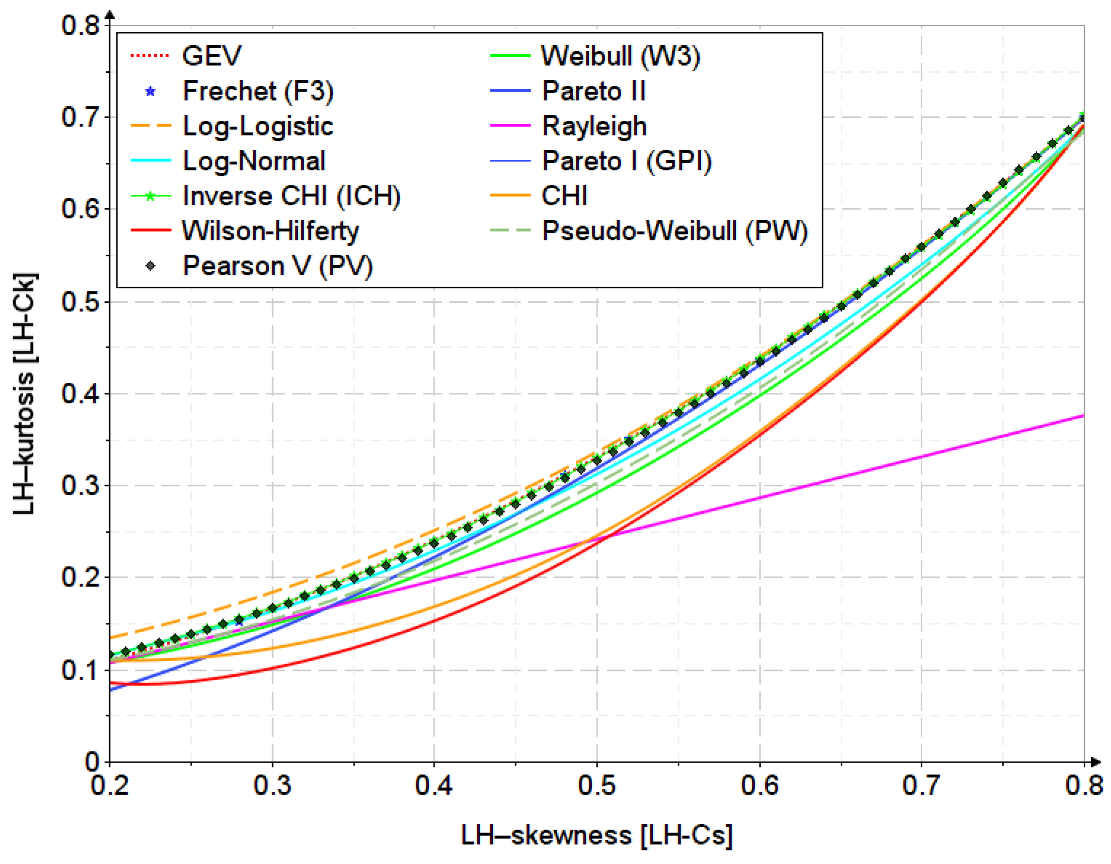
Appendix D. The Second-Order LH-Moments Diagram

In the next section, the variation in the second-order LH-kurtosis depending on the positive second-order LH-skewness is presented for certain theoretical distributions often used in hydrology and in this article.

Figure A3. The variation diagram for the second-order LH-skewness and LH-kurtosis.

Log-normal:

\begin{array}{l} τ_{H 4} = - 0 . 5839924 + 11 . 4481002 \cdot τ_{H 3} - 80 . 7815681 \cdot τ_{H 3}^{2} + 312 . 6958061 \cdot τ_{H 3}^{3} - 693 . 2943739 \cdot τ_{H 3}^{4} + \\ 891 . 9112256 \cdot τ_{H 3}^{5} - 617 . 8611695 \cdot τ_{H 3}^{6} + 178 . 3238894 \cdot τ_{H 3}^{7} \end{array}

GEV:

\begin{array}{l} τ_{H 4} = 0 . 0482673 + 0 . 1356835 \cdot τ_{H 3} + 0 . 871055 \cdot τ_{H 3}^{2} - 0 . 0306327 \cdot τ_{H 3}^{3} - 0 . 0006064 \cdot τ_{H 3}^{4} + \\ 0 . 0078749 \cdot τ_{H 3}^{5} - 0 . 0043548 \cdot τ_{H 3}^{6} + 0 . 0002965 \cdot τ_{H 3}^{7} \end{array}

Weibull:

\begin{array}{l} τ_{H 4} = 0 . 0752617 + 0 . 1485934 \cdot τ_{H 3} - 1 . 4212834 \cdot τ_{H 3}^{2} + 13 . 37326 \cdot τ_{H 3}^{3} - 42 . 2993121 \cdot τ_{H 3}^{4} + \\ 75 . 3056365 \cdot τ_{H 3}^{5} - 69 . 4800457 \cdot τ_{H 3}^{6} + 25 . 8473539 \cdot τ_{H 3}^{7} \end{array}

Rayleigh:

τ_{H 4} = \frac{63 \cdot τ_{H 3} - 20}{6} - \frac{14 \cdot (10 \cdot \sqrt{6} + \sqrt{3} - 8 \cdot \sqrt{2} - 15) \cdot (3 \cdot τ_{H 3} - 1)}{9 \cdot \sqrt{10} + 54 \cdot \sqrt{6} - 60 \cdot \sqrt{2} - 72}

Log-logistic:

τ_{H 4} = \frac{2016 \cdot τ_{H 3}^{2} + 105 \cdot τ_{H 3} + 200}{2250}

Fréchet:

\begin{array}{l} τ_{H 4} = 0 . 033874 + 0 . 2724765 \cdot τ_{H 3} + 0 . 4979464 \cdot τ_{H 3}^{2} - 0 . 3498839 \cdot τ_{H 3}^{3} + 3 . 6272441 \cdot τ_{H 3}^{4} - \\ 7 . 4671598 \cdot τ_{H 3}^{5} + 6 . 602143 \cdot τ_{H 3}^{6} - 2 . 1982501 \cdot τ_{H 3}^{7} \end{array}

Pearson V:

\begin{array}{l} τ_{H 4} = 0 . 249419 - 3 . 2415526 \cdot τ_{H 3} + 26 . 1472533 \cdot τ_{H 3}^{2} - 104 . 7386881 \cdot τ_{H 3}^{3} + 253 . 0618092 \cdot τ_{H 3}^{4} - \\ 354 . 2485544 \cdot τ_{H 3}^{5} + 265 . 8319905 \cdot τ_{H 3}^{6} - 82 . 6153103 \cdot τ_{H 3}^{7} \end{array}

Pseudo-Weibull:

\begin{array}{l} τ_{H 4} = 0 . 3121672 - 4 . 5110186 \cdot τ_{H 3} + 36 . 6833749 \cdot τ_{H 3}^{2} - 153 . 3360061 \cdot τ_{H 3}^{3} + 380 . 7876839 \cdot τ_{H 3}^{4} - \\ 546 . 2031254 \cdot τ_{H 3}^{5} + 419 . 1284756 \cdot τ_{H 3}^{6} - 132 . 8075228 \cdot τ_{H 3}^{7} \end{array}

Wilson–Hilferty:

\begin{array}{l} τ_{H 4} = 0 . 8041465 - 11 . 1539365 \cdot τ_{H 3} + 70 . 1801786 \cdot τ_{H 3}^{2} - 236 . 6915869 \cdot τ_{H 3}^{3} + 467 . 3353544 \cdot τ_{H 3}^{4} - \\ 526 . 1946551 \cdot τ_{H 3}^{5} + 311 . 3745049 \cdot τ_{H 3}^{6} - 74 . 1049756 \cdot τ_{H 3}^{7} \end{array}

CHI:

\begin{array}{l} τ_{H 4} = - 0 . 1619727 + 6 . 0051765 \cdot τ_{H 3} - 52 . 2568473 \cdot τ_{H 3}^{2} + 232 . 1939653 \cdot τ_{H 3}^{3} - 577 . 2377642 \cdot τ_{H 3}^{4} + \\ 827 . 685701 \cdot τ_{H 3}^{5} - 634 . 4947449 \cdot τ_{H 3}^{6} + 201 . 0426143 \cdot τ_{H 3}^{7} \end{array}

Inverse CHI:

\begin{array}{l} τ_{H 4} = 0 . 0083177 + 1 . 4215276 \cdot τ_{H 3} - 11 . 199805 \cdot τ_{H 3}^{2} + 55 . 2535502 \cdot τ_{H 3}^{3} - 141 . 758711 \cdot τ_{H 3}^{4} + \\ 207 . 6688672 \cdot τ_{H 3}^{5} - 162 . 1766982 \cdot τ_{H 3}^{6} + 52 . 284264 \cdot τ_{H 3}^{7} \end{array}

Generalized Pareto Type I:

τ_{H 4} = \frac{21 \cdot τ_{H 3} - 240}{2} + \frac{4200}{3 \cdot τ_{H 3} + 35}

Appendix E. Estimation of the Frequency Factor for the PV Distribution

The frequency factor for L-moments can be estimated using the following polynomial function:

K_{p} (p) = a + b \cdot τ_{3} + c \cdot τ_{3}^{2} + d \cdot τ_{3}^{3} + e \cdot τ_{3}^{4} + f \cdot τ_{3}^{5} + g \cdot τ_{3}^{6} + h \cdot τ_{3}^{7}

Table A2. The frequency factor for estimation with L-moments for PV distribution.

P (%)	a	b	c	d	e	f	g	h
0.01	11.25716	−131.20350	1949.68567	−11,151.25939	37,380.04905	−68,646.56566	70,412.75359	−29,839.17905
0.1	5.95329	5.28685	105.58814	−116.64929	−37.55278	1085.44951	−1235.53789	185.05204
0.5	5.20696	−6.34402	171.13982	−663.09642	1552.89993	−1826.49212	975.79402	−210.37970
1	4.67849	−6.34289	145.23208	−593.97206	1402.57612	−1769.23389	1073.27459	−257.35685
2	4.09166	−5.72542	113.45047	−479.90312	1119.04640	−1438.61769	917.93954	−231.36365
3	3.72488	−5.34813	95.45312	−411.10312	948.26394	−1217.30511	786.82014	−201.56570
5	3.23329	−4.91688	74.39560	−328.29622	747.90220	−951.38916	618.18166	−160.15142
10	2.49248	−4.33153	48.49037	−222.21910	502.38567	−628.82146	406.76300	−105.78320
20	1.61367	−3.50095	24.39044	−116.57543	265.83072	−329.17366	211.21241	−54.80899
40	0.46069	−1.90237	0.28296	−2.20461	6.47671	−7.31658	4.39076	−1.18922
50	−0.02947	−1.00147	−8.04637	38.61740	−88.73004	111.53103	−71.90978	18.57044
80	−1.63651	3.08779	−30.87890	144.26162	−339.62037	429.40736	−277.82412	72.21398
90	−2.46681	5.99191	−42.14745	187.59670	−439.64825	556.34369	−360.55393	93.89877

The frequency factor for the first-order LH-moments can be estimated using the following polynomial function:

K_{p} (p) = a + b \cdot τ_{3 H} + c \cdot τ_{3 H}^{2} + d \cdot τ_{3 H}^{3} + e \cdot τ_{3 H}^{4} + f \cdot τ_{3 H}^{5} + g \cdot τ_{3 H}^{6} + h \cdot τ_{3 H}^{7}

Table A3. The frequency factor for estimation with LH-moments for PV distribution.

P (%)	a	b	c	d	e	f	g	h
0.01	81.910475	−1771.514355	16,819.397533	−82,805.460187	235,276.652260	−386,190.499025	346,280.769342	−130,055.21879
0.1	2.228731	59.123754	−391.394621	1911.377627	−4602.449696	6513.540173	−4024.546602	352.304188
0.5	3.512205	12.804180	−28.860341	198.686814	−458.874164	782.400511	−811.234773	272.458238
1	3.314992	7.768633	−2.463356	39.354768	−38.467754	15.733888	−88.865312	49.856120
2	2.925506	5.809312	−5.173311	30.048369	−37.998837	−28.905010	31.467196	−5.026159
3	2.655839	4.814207	−8.278126	36.412452	−73.682802	34.281005	1.400566	−2.325368
5	2.277429	3.322797	−9.645991	35.521977	−91.128870	89.977174	−41.449511	8.012619
10	1.656367	1.012819	−7.248799	18.654250	−56.540573	76.866583	−48.609237	12.214375
20	0.806822	−1.031876	−3.526086	2.999739	−6.727668	15.136075	−13.329765	4.178605
40	−0.520195	−2.007167	0.079953	0.896835	5.241720	−10.751092	7.944665	−2.160109
50	−1.161667	−1.793933	1.853417	−0.018740	3.201880	−8.323464	7.222178	−2.214021
80	−3.651550	2.664287	5.060010	−17.180213	27.188778	−26.520914	14.982105	−3.714598
90	−5.224593	8.397516	−2.422149	−17.374685	41.178694	−46.186319	27.185834	−6.714774

Appendix F. Estimation of the Frequency Factor for the ICH Distribution

The frequency factor for L-moments can be estimated using the following polynomial function:

K_{p} (p) = a + b \cdot τ_{3} + c \cdot τ_{3}^{2} + d \cdot τ_{3}^{3}

Table A4. The frequency factor for estimation with L-moments for ICH distribution.

P (%)	a	b	c	d
0.01	6.52997	26.82067	14.85657	464.96943
0.1	5.44941	17.20176	11.39250	177.19999
0.5	4.55112	11.16190	4.43462	72.13282
1	4.11304	8.70764	1.40446	44.77481
2	3.63324	6.34343	−1.21804	25.78376
3	3.32837	5.00664	−2.44115	17.89105
5	2.91207	3.38007	−3.53519	10.69300
10	2.27033	1.30825	−3.99266	4.64115
20	1.49234	−0.51235	−2.92430	1.11878
40	0.45076	−1.78115	0.04530	−2.15319
50	0.00178	−1.91764	1.40809	−3.60146
80	−1.49132	−0.60439	3.68532	−7.00379
90	−2.27256	1.15360	2.18165	−5.73713

The frequency factor for the first-order LH-moments can be estimated using the following polynomial function:

K_{p} (p) = a + b \cdot τ_{3 H} + c \cdot τ_{3 H}^{2} + d \cdot τ_{3 H}^{3} + e \cdot τ_{3 H}^{4} + f \cdot τ_{3 H}^{5} + g \cdot τ_{3 H}^{6} + h \cdot τ_{3 H}^{7}

Table A5. The frequency factor for estimation with LH-moments for ICH distribution.

P (%)	a	b	c	d	e	f	g	h
0.01	79.883758	−1679.417954	15,661.299605	−76,196.141845	215,236.713	−351,779.05466	315,145.61355	−118,719.36587
0.1	2.439485	54.257459	−349.512901	1696.329214	−3847.028237	5154.772004	−2931.225766	45.180979
0.5	3.640380	11.167621	−27.074245	238.032175	−608.858332	991.975375	−943.188586	306.114622
1	3.513630	4.477591	14.966696	9.106453	−49.568623	100.765426	−176.345385	79.786789
2	3.146844	1.734343	22.157049	−55.650510	94.739536	−129.454331	62.029820	−5.334231
3	2.864035	0.848887	20.078952	−62.468499	105.677263	−139.464427	86.184870	−18.314985
5	2.447099	0.004927	15.332281	−58.814530	98.385355	−117.730239	76.491903	−19.179270
10	1.753158	−0.896712	7.695230	−41.884058	75.958313	−82.338902	50.779609	−13.064095
20	0.834726	−1.534456	0.288985	−13.264633	32.253908	−36.485557	21.964914	−5.564021
40	−0.531047	−1.730709	−2.509832	12.719488	−22.304466	23.482121	−13.881077	3.482139
50	−1.176148	−1.474153	−0.968034	12.970906	−28.143980	32.298762	−19.777144	5.041014
80	−3.667051	2.829186	4.750684	−19.036152	35.510723	−39.892243	24.957853	−6.634231
90	−5.248541	8.651554	−2.624214	−24.417599	70.138835	−93.925739	63.986862	−17.749432

Appendix G. Estimation of the Frequency Factor for the LN3 Distribution

The frequency factor for L-moments can be estimated using a rational function:

K_{p} (p) = \frac{a + b \cdot τ_{3} + c \cdot τ_{3}^{2} + d \cdot τ_{3}^{3} + e \cdot τ_{3}^{4} + f \cdot τ_{3}^{5} + g \cdot τ_{3}^{6}}{1 + h \cdot τ_{3} + i \cdot τ_{3}^{2} + j \cdot τ_{3}^{3}}

Table A6. The frequency factor for estimation with L-moments for Log-normal distribution.

P (%)	a	b	c	d	e	f	g	h	i
0.01	7.34577	−11.93543	716.47126	−4366.76433	13,233.45376	−17,502.29426	9087.37090	0.13890	−0.31483
0.1	−182.8854	80,948.57367	69,705.91443	29,162.82665	−47,509.61155	−40,863.74927	−86,394.5813	13,007.97382	−22,817.9312
0.5	4.46079	768.03648	392.38804	2614.73022	−5453.94909	4471.71101	−2769.46863	161.69088	−188.52368
1	5.05392	3381.94490	4190.83018	1683.11151	−4342.06310	−1032.28092	−3834.14862	828.61007	−638.47665
2	3.72540	559.11509	678.67334	283.47264	−1231.65344	218.68686	−530.59615	152.94462	−60.42997
3	3.34676	268.95983	249.09931	62.99081	−578.86038	94.48113	−119.72659	79.34274	−32.25046
5	2.90555	3.51178	−4.44349	21.53572	−56.29603	59.07715	−27.31915	−0.00055	0.00201
10	2.27392	10.31129	0.12209	−25.46670	15.97668	−30.11238	26.69439	4.08106	−2.17704
20	1.47852	1457.8469	−918.40881	−2278.41631	−529.77821	2130.23329	−102.47085	977.02214	−257.24175
40	0.44943	−1.71341	−0.58245	−0.17569	2.15788	−1.99608	0.85851	−	−
50	−0.00005	−1.81172	−0.02237	0.94326	−0.20718	0.17417	−0.07598	−	−
80	−1.49191	−0.52177	1.78568	−0.41759	−0.93231	0.93656	−0.35804	−	−
90	−2.27165	1.17186	1.28540	−1.61220	0.18629	0.49903	−0.25817	−	−

The frequency factor for LH-moments can be estimated using a polynomial function:

K_{p} (p) = a + b \cdot τ_{H 3} + c \cdot τ_{H 3}^{2} + d \cdot τ_{H 3}^{3} + e \cdot τ_{H 3}^{4}

Table A7. The frequency factor for estimation with LH-moments for Log-normal distribution.

P (%)	a	b	c	d
0.01	20.4560566	0.0157214	7.6751191	0.1690430
0.1	19.9223136	0.0157565	7.7306869	0.1694185
0.5	19.4863608	0.0157853	7.7760593	0.1697253
1	19.2751529	0.0157992	7.7980364	0.1698740
2	19.0445424	0.0158144	7.8220289	0.1700363
3	18.8983187	0.0158240	7.8372399	0.1701393
5	18.6989591	0.0158372	7.8579761	0.1702796
10	18.3922410	0.0158574	7.8898737	0.1704956
20	18.0212465	0.0158819	7.9284472	0.1707569
40	17.5258663	0.0159145	7.9799386	0.1711059
50	17.3127762	0.0159286	8.0020827	0.1712560
80	16.6059721	0.0159752	8.0755103	0.1717541
90	16.2371749	0.0159996	8.1138096	0.1720141

Appendix H. Estimation of the Frequency Factor for the FR Distribution

The frequency factor for L-moments can be estimated using a rational function:

K_{p} (p) = \frac{a + b \cdot τ_{3}}{1 + c \cdot τ_{3} + d \cdot τ_{3}^{2} + e \cdot τ_{3}^{3} + f \cdot τ_{3}^{4} + g \cdot τ_{3}^{5} + h \cdot τ_{3}^{6}}

Table A8. The frequency factor for estimation with L-moments for FR distribution.

P (%)	a	b	c	d	e	f	g	h
0.01	4.79878	−4.79613	−6.32125	17.28586	−25.92369	22.32216	−10.40520	2.04267
0.1	4.60163	−4.60769	−4.90472	10.51612	−12.27707	7.99307	−2.64179	0.31910
0.5	4.22930	−4.25399	−3.71518	5.66451	−3.27906	−1.32316	2.62737	−0.95280
1	3.91982	−3.96379	−3.31247	4.71382	−2.66524	−0.95161	1.98933	−0.73158
2	3.54772	−3.62982	−2.86477	3.75946	−2.06788	−0.65905	1.46457	−0.55126
3	3.29251	−3.41148	−2.58280	3.23198	−1.80321	−0.41053	1.11661	−0.43379
5	2.92396	−3.11434	−2.19334	2.52840	−1.27243	−0.51770	1.05146	−0.40659
10	2.31559	−2.67844	−1.61581	1.72570	−0.89911	−0.20951	0.61552	−0.25426
20	1.53537	−2.24054	−0.93998	1.02318	−0.49957	−0.06099	0.30917	−0.12674
40	0.45853	−1.89670	−0.07881	0.41672	0.13819	−0.05952	−0.06296	0.08501
50	−0.00696	−1.84955	0.26139	0.40009	0.16243	0.00554	−0.01990	0.04712
80	−1.52193	0.01607	−0.14440	0.92152	−0.44753	0.00190	0.33891	−0.16508
90	−2.28341	1.29295	0.04646	0.24771	−0.28723	−0.06346	0.06346	−0.05894

The frequency factor for LH-moments can be estimated using a polynomial function:

K_{p} (p) = a + b \cdot τ_{H 3} + c \cdot τ_{H 3}^{2} + d \cdot τ_{H 3}^{3} + e \cdot τ_{H 3}^{4}

Table A9. The frequency factor for estimation with LH-moments for FR distribution.

P (%)	a	b	c	d
0.01	20.4560566	0.0157214	7.6751191	0.1690430
0.1	19.9223136	0.0157565	7.7306869	0.1694185
0.5	19.4863608	0.0157853	7.7760593	0.1697253
1	19.2751529	0.0157992	7.7980364	0.1698740
2	19.0445424	0.0158144	7.8220289	0.1700363
3	18.8983187	0.0158240	7.8372399	0.1701393
5	18.6989591	0.0158372	7.8579761	0.1702796
10	18.3922410	0.0158574	7.8898737	0.1704956
20	18.0212465	0.0158819	7.9284472	0.1707569
40	17.5258663	0.0159145	7.9799386	0.1711059
50	17.3127762	0.0159286	8.0020827	0.1712560
80	16.6059721	0.0159752	8.0755103	0.1717541
90	16.2371749	0.0159996	8.1138096	0.1720141

Appendix I. The Probability Density Functions and Complementary Cumulative Distribution Function

In Table A10, the probability density function

f (x)

and the complementary cumulative distribution function

F (x)

for the analyzed distributions are presented [20,21,31,32].

Table A10. The probability density functions and complementary cumulative distribution function.

Distribution	$f (x)$	$F (x)$
PV	$\frac{\exp (- \frac{β}{x - γ})}{β \cdot Γ (α - 1)} \cdot {(\frac{x - γ}{β})}^{- α}$	$1 - \int_{γ}^{x} \frac{\exp (- \frac{β}{x - γ})}{β \cdot Γ (α - 1)} \cdot {(\frac{x - γ}{β})}^{- α} d x = \frac{Γ (α - 1, \frac{β}{x - γ})}{Γ (α - 1)}$
CHI	$\frac{{(\frac{x - γ}{β})}^{α - 1}}{2^{\frac{α}{2} - 1} \cdot β \cdot Γ (\frac{α}{2})} \cdot \exp (- \frac{{(x - γ)}^{2}}{2 \cdot β^{2}})$	$1 - \int_{γ}^{x} \frac{{(\frac{x - γ}{β})}^{α - 1}}{2^{\frac{α}{2} - 1} \cdot β \cdot Γ (\frac{α}{2})} \cdot \exp (- \frac{{(x - γ)}^{2}}{2 \cdot β^{2}}) d x = \frac{Γ (\frac{α}{2}, \frac{{(x - γ)}^{2}}{2 \cdot β^{2}})}{Γ (\frac{α}{2})}$
ICH	$\frac{2 \cdot \exp (- {(\frac{β}{x - γ})}^{2})}{\|β\| \cdot Γ (α)} \cdot {(\frac{β}{x - γ})}^{2 \cdot α + 1}$	$1 - \int_{γ}^{x} \frac{2 \cdot \exp (- {(\frac{β}{x - γ})}^{2})}{\|β\| \cdot Γ (α)} \cdot {(\frac{β}{x - γ})}^{2 \cdot α + 1} d x = \frac{Γ (α, {(\frac{β}{x - γ})}^{2})}{Γ (α)}$
WH	$\frac{3 \cdot \exp (- {(\frac{x - γ}{β})}^{3})}{\|β\| \cdot Γ (α)} \cdot {(\frac{x - γ}{β})}^{3 \cdot α - 1}$	$1 - \int_{γ}^{x} \frac{3 \cdot \exp (- {(\frac{x - γ}{β})}^{3})}{\|β\| \cdot Γ (α)} \cdot {(\frac{x}{β})}^{3 \cdot α - 1} d x = \frac{Γ (α, {(\frac{x - γ}{β})}^{3})}{Γ (α)}$
PW	$\frac{1}{Γ (1 + \frac{1}{α})} \cdot \|\frac{α}{β}\| \cdot {(\frac{x - γ}{β})}^{α} \cdot \exp (- {(\frac{x - γ}{β})}^{α})$	$\begin{array}{l} 1 - \int_{γ}^{x} \frac{1}{Γ (1 + \frac{1}{α})} \cdot \|\frac{α}{β}\| \cdot {(\frac{x - γ}{β})}^{α} \cdot \exp (- {(\frac{x - γ}{β})}^{α}) d x = \\ = \frac{Γ (\frac{1}{α} + 1, {(\frac{x - γ}{β})}^{α})}{Γ (\frac{1}{α} + 1)} \end{array}$
LN3	$\frac{\exp (- \frac{{(\ln (x - γ) - α)}^{2}}{2 \cdot β^{2}})}{(x - γ) \cdot β \cdot \sqrt{2 \cdot π}}$ $\frac{1}{x - γ} \cdot d n o r m (\ln (x - γ), α, β)$ $d l n o r m (x - γ, α, β)$	$1 - \frac{1}{2} \cdot (e r f (\frac{(\ln (x - γ) - α)}{\sqrt{2} \cdot β}) + 1)$ $1 - p n o r m (\ln (x - γ), α, β) = 1 - p l n o r m (x - γ, α, β)$ $1 - c n o r m (\frac{\ln (x - γ) - α}{β})$
GPI	$\frac{α}{β} \cdot {(\frac{x - γ}{β})}^{- α - 1}$	${(\frac{x - γ}{β})}^{- α}$
FR	$\frac{α}{β} \cdot {(\frac{x - γ}{β})}^{- α - 1} \cdot \exp (- {(\frac{x - γ}{β})}^{- α})$	$1 - \exp (- {(\frac{x - γ}{β})}^{- α})$

Appendix J. The Confidence Intervals of the Analysed Distributions

Figure A4 presents the results of the analysed distributions, highlighting the confidence interval (C.I) for each distribution for both parameter estimation methods.

Figure A4. The probability distribution curves with confidence intervals.

The confidence interval for each distribution was established based on Chow’s relation [3,18], which, until recently [24,25,26], was exclusively used for parameter estimation using the method of ordinary moments. This is based on a Gaussian assumption, using the frequency factor and the desired confidence level.

Appendix K. Built-In Function in Mathcad

Γ (α) = \int_{0}^{\infty} t^{α - 1} \cdot e^{- t} d t

the complete gamma function.

Γ (α, x) = \int_{x}^{\infty} t^{α - 1} \cdot e^{- t} d t

returns the value of the upper incomplete gamma function of x with parameter

α

.

q g a m m a (p, α) = Γ^{- 1} (p; α)

returns the inverse cumulative probability distribution for probability p for the Gamma distribution.

d n o r m (x, α, β)

—returns the probability density for value x for normal distribution.

p n o r m (x, α, β)

—returns the cumulative probability distribution for value x for normal distribution.

q n o r m (p, 0, 1)

—returns the inverse standard cumulative probability distribution for probability p for normal distribution.

c n o r m (x)

—returns the cumulative probability distribution with mean 0 and variance 1 for normal distribution.

d l n o r m (x, α, β)

—returns the probability density for value x for Log-normal distribution.

p l n o r m (x, α, β)

—returns the cumulative probability distribution for value x for Log-normal distribution.

q l n o r m (p, μ, σ)

—returns the inverse cumulative probability distribution for probability p for Log-normal distribution.

e r f (x)

—returns the error function.

References

Wang, Q.J. LH moments for statistical analysis of extreme events. Water Resour. Res. 1997, 33, 2841–2848. [Google Scholar] [CrossRef]
Hosking, J.R.M.; Wallis, J.R. Regional Frequency Analysis: An Approach Based on L–Moments; Cambridge University Press: Cambridge, UK, 1997. [Google Scholar] [CrossRef]
Rao, A.R.; Hamed, K.H. Flood Frequency Analysis; CRC Press LLC: Boca Raton, FL, USA, 2000. [Google Scholar]
Greenwood, J.A.; Landwehr, J.M.; Matalas, N.C.; Wallis, J.R. Probability Weighted Moments: Definition and Relation to Parameters of Several Distributions Expressable in Inverse Form. Water Resour. Res. 1979, 15, 1049–1054. [Google Scholar] [CrossRef]
Hosking, J.R.M. L–moments: Analysis and Estimation of Distributions using Linear, Combinations of Order Statistics. J. R. Statist. Soc. 1990, 52, 105–124. [Google Scholar] [CrossRef]
Houghton, J.C. Birth of a parent: The Wakeby distribution for modeling flood flows. Water Resour. Res. 1978, 14, 1105–1109. [Google Scholar] [CrossRef]
Hewa, G.A.; Wang, Q.J.; McMahon, T.A.; Nathan, R.J.; Peel, M.C. Generalized extreme value distribution fitted by LH moments for low–flow frequency analysis. Water Resour. Res. 2007, 43, W06301. [Google Scholar] [CrossRef]
Wang, Q.J. Approximate Goodness–of–Fit Tests of fitted generalized extreme value distributions using LH moments. Water Resour. Res. 1998, 34, 3497–3502. [Google Scholar] [CrossRef]
Fawad, M.; Cassalho, F.; Ren, J.; Chen, L.; Yan, T. State–of–the–Art Statistical Approaches for Estimating Flood Events. Entropy 2022, 24, 898. [Google Scholar] [CrossRef]
Lee, S.H.; Maeng, S.J. Comparison and analysis of design floods by the change in the order of LH–moment methods. Irrig. Drain. 2003, 52, 231–245. [Google Scholar] [CrossRef]
Meshgi, A.; Khalili, D. Comprehensive evaluation of regional flood frequency analysis by L– and LH–moments. II. Development of LH–moments parameters for the generalized Pareto and generalized logistic distributions. Stoch. Environ. Res. Risk Assess. 2009, 23, 137–152. [Google Scholar] [CrossRef]
Meshgi, A.; Khalili, D. Comprehensive evaluation of regional flood frequency analysis by L– and LH–moments. I. A revisit to regional homogeneity. Stoch. Environ. Res. Risk Assess. 2009, 23, 119–135. [Google Scholar] [CrossRef]
Bhuyan, A.; Borah, M.; Kumar, R. Regional Flood Frequency Analysis of North–Bank of the River Brahmaputra by Using LH–Moments. Water Resour. Manag. 2010, 24, 1779–1790. [Google Scholar] [CrossRef]
Nouri Gheidari, M.H. Comparisons of the L– and LH–moments in the selection of the best distribution for regional flood frequency analysis in Lake Urmia Basin. Civ. Eng. Environ. Syst. 2013, 30, 72–84. [Google Scholar] [CrossRef]
Deka, S.; Borah, M.; Kakaty, S.C. Statistical analysis of annual maximum rainfall in North–East India: An application of LH–moments. Theor. Appl. Climatol. 2011, 104, 111–122. [Google Scholar] [CrossRef]
Zakaria, Z.; Suleiman, J.; Mohamad, M. Rainfall frequency analysis using LH–moments approach: A case of Kemaman Station, Malaysia. Int. J. Eng. Technol. 2018, 7, 107–110. [Google Scholar] [CrossRef]
Bora, D.J.; Borah, M.; Bhuyan, A. Regional analysis of maximum rainfall using L–moment and LH–moment: A comparative case study for the northeast India. Mausam 2017, 68, 451–462. [Google Scholar] [CrossRef]
Ilinca, C.; Anghel, C.G. Flood–Frequency Analysis for Dams in Romania. Water 2022, 14, 2884. [Google Scholar] [CrossRef]
Anghel, C.G.; Ilinca, C. Hydrological Drought Frequency Analysis in Water Management Using Univariate Distributions. Appl. Sci. 2023, 13, 3055. [Google Scholar] [CrossRef]
Ilinca, C.; Anghel, C.G. Flood Frequency Analysis Using the Gamma Family Probability Distributions. Water 2023, 15, 1389. [Google Scholar] [CrossRef]
Anghel, C.G.; Ilinca, C. Parameter Estimation for Some Probability Distributions Used in Hydrology. Appl. Sci. 2022, 12, 12588. [Google Scholar] [CrossRef]
Md Sharwar, M.; Park, B.-J.; Jeong, B.-Y.; Park, J.-S. LH–Moments of Some Distributions Useful in Hydrology. Commun. Stat. Appl. Methods 2009, 16, 647–658. [Google Scholar]
Gaume, E. Flood frequency analysis: The Bayesian choice. WIREs Water. 2018, 5, e1290. [Google Scholar] [CrossRef]
Chow, V.T.; Maidment, D.R.; Mays, L.W. Applied Hydrology; McGraw–Hill, Inc.: New York, NY, USA, 1988; ISBN 007-010810-2. [Google Scholar]
Bulletin 17B Guidelines for Determining Flood Flow Frequency; Hydrology Subcommittee; Interagency Advisory Committee on Water Data; U.S. Department of the Interior; U.S. Geological Survey; Office of Water Data Coordination: Reston, VA, USA, 1981.
Bulletin 17C Guidelines for Determining Flood Flow Frequency; U.S. Department of the Interior; U.S. Geological Survey: Reston, VA, USA, 2017.
Anghel, C.G.; Ilinca, C. Evaluation of Various Generalized Pareto Probability Distributions for Flood Frequency Analysis. Water 2023, 15, 1557. [Google Scholar] [CrossRef]
Ministry of the Environment. The Romanian Water Classification Atlas, Part I—Morpho–Hydrographic Data on the Surface Hydrographic Network; Ministry of the Environment: Bucharest, Romania, 1992. [Google Scholar]
Teodorescu, I.; Filotti, A.; Chiriac, V.; Ceausescu, V.; Florescu, A. Water Management; Ceres Publishing House: Bucharest, Romania, 1973. [Google Scholar]
Ilinca, C.; Anghel, C.G. Frequency Analysis of Extreme Events Using the Univariate Beta Family Probability Distributions. Appl. Sci. 2023, 13, 4640. [Google Scholar] [CrossRef]
Zhao, F.; Wang, X.; Wu, Y.; Singh, S.K. Prefectures vulnerable to water scarcity are not evenly distributed across China. Commun. Earth Environ. 2023, 4, 145. [Google Scholar] [CrossRef]
Zhao, F.; Wang, X.; Wu, Y.; Sivakumar, B.; Liu, S. Enhanced Dependence of China’s Vegetation Activity on Soil Moisture Under Drier Climate Conditions. J. Geophys. Res. Biogeosci. 2023, 128, e2022JG007300. [Google Scholar] [CrossRef]

Figure 1. The flow chart describing the methodological approach.

Figure 2. The Prigor River location, Danube watershed, Romania.

Figure 3. Evaluations of the quantile function for the two methods of parameter estimation.

Figure 4. Variation in the shape parameter for the two methods.

Figure 5. The skewness–kurtosis variation for the two parameter estimation methods.

Table 1. Novelty elements.

New Elements	Method of Parameter Estimation
New Elements	LH−Moments
Exact parameter estimation	PV, CHI, ICH, WH, PW, PGI, FR
Approximate estimation of parameters	PV, CHI, ICH, WH, PW, PGI, FR, LN3
Expression of the inverse function with the frequency factor	PV, CHI, ICH, WH, PW, PGI, FR
Exact relationships of the frequency factors	PV, CHI, ICH, WH, PW, PGI, FR
Approximate estimation of the frequency factors	PV, CHI, ICH, WH, PW, PGI, FR
The confidence interval with Chow’s relationship	PV, CHI, ICH, WH, PW, PGI, FR
The skewness−kurtosis variation graph and relationships	PV, CHI, ICH, WH, PW, PGI, FR

Table 2. The analyzed probability distributions.

Distribution	$x (p)$	Distribution	$x (p)$
PV	$γ + \frac{β}{q g a m m a (p, α - 1)}$	WH	$γ + β \cdot q g a m m a {(1 - p, α)}^{\frac{1}{3}}$
CHI	$γ + β \cdot \sqrt{2 \cdot g a m m a (1 - p, \frac{α}{2})}$	PW	$γ + β \cdot q g a m m a {(1 - p, (\frac{1}{α} + 1))}^{\frac{1}{α}}$
LN3	$γ + \exp (α + β \cdot q n o r m (1 - p, 0, 1))$ $γ + q l n o r m (1 - p, α, β)$	ICH	$γ + \frac{β}{q g a m m a {(p, α)}^{\frac{1}{2}}}$
PGI	$γ + β \cdot p^{- \frac{1}{α}}$	FR	$γ + β \cdot {(- \ln (1 - p))}^{- 1 / α}$

Table 3. The morphometric indicators of the Prigor River.

Length (km)	Average Stream Slope (‰)	Sinuosity Coefficient (−)	Average Altitude (m)	Watershed Area (km²)
33	22	1.83	713	153

Table 4. The observed data from the Prigor River.

AMS
		1990	1991	1992	1993	1994	1995	1996	1997	1998	1999	2000
Flow	(m³/s)	9.96	15	10.1	14.8	7.30	21.2	18.2	21.4	13.1	14.5	35
		2001	2002	2003	2004	2005	2006	2007	2008	2009	2010	2011
Flow	(m³/s)	19.9	22.1	11.8	80.3	88	51.6	72.2	16.2	42.6	28.5	12.8
		2012	2013	2014	2015	2016	2017	2018	2019	2020
Flow	(m³/s)	31.2	24.1	52.2	21.1	18.9	6.40	24.9	15.1	36.6

Table 5. The statistical indicators of the data series for the L-moments and LH-moments.

Prigor River	Statistical Indicators
	L-moments
	$L_{1}$	$L_{2}$	$L_{3}$	$L_{4}$	$τ_{2}$	$τ_{3}$	$τ_{4}$
	(m³/s)	(m³/s)	(m³/s)	(m³/s)	(−)	(−)	(−)
	27.2	10.7	4.26	2.43	0.386	0.399	0.228
	LH-moments (first order)
	$L_{H 1}$	$L_{H 2}$	$L_{H 3}$	$L_{H 4}$	$τ_{H 2}$	$τ_{H 3}$	$τ_{H 4}$
	(m³/s)	(m³/s)	(m³/s)	(m³/s)	(−)	(−)	(−)
	38.3	11.2	4.46	1.99	0.292	0.398	0.177

Table 6. Quantile results for the two methods of parameter estimation.

Distr.	Annual Maximum Series (AMS)
	Exceedance Probabilities (%)
	L-Moments									LH-Moments (First Order)
	0.01	0.1	0.5	1	2	3	5	80	90	0.01	0.1	0.5	1	2	3	5	80	90
PV	562	270	159	125	97.2	83.6	68.5	12.4	9.63	467	244	151	121	96.5	83.7	69.4	11.4	8.16
CHI	165	137	114	103	90.9	83.4	73.4	11.1	10.4	178	147	121	108	94.9	86.4	75.1	13.4	13.2
ICH	624	284	162	126	97.5	83.5	68.2	12.4	9.46	498	251	152	122	96.2	83.3	70	11.4	7.94
WH	139	121	106	97.4	88.2	82.1	73.5	11.2	10.7	152	131	113	104	93.2	86.1	76.1	13.9	13.8
PW	292	198	141	118	97.4	85.8	72	11.8	9.64	297	200	142	119	97.7	86	72	11.9	9.82
LN3	480	266	165	132	103	87.9	71.4	12.4	10.3	367	222	147	121	97.4	85	70.7	11.6	8.88
GPI	329	207	142	118	96.8	85.1	71.4	11.7	9.60	340	211	144	119	97.1	85.2	71.3	11.8	9.76
FR	623	285	162	126	97.7	83.6	68.2	12.4	9.47	489	250	152	122	96.3	83.5	69	11.4	7.90

Table 7. Parameters estimated using the L-moments and LH-moments methods for Prigor River.

Annual Maximum Series (AMS)
Parameters	Distribution
Parameters	PV	CHI	ICH	WH	PW	LN3	GPI	FR
L-moments
$α$	4.3055	0.3887	1.5005	0.1099	0.5467	2.601	7.1344	3.0516
$β$	69.4	44.4	32.3	73.2	2.41	0.9569	122	31.2
$γ$	−2.46	10.3	−8.83	10.7	7.23	6.34	−114	−14.2
LH-moments (first order)
$α$	4.8615	0.2929	1.7617	0.081	0.5375	2.894	6.6853	3.6925
$β$	98.2	48.7	43.2	80.1	2.24	0.8072	112	42.5
$γ$	−6.95	13.2	−15.04	13.8	7.52	2.47	−104	−26.03

Table 8. Distribution performance values.

Distr.	Statistical Measures
	Methods of Parameter Estimation								Observed Data
	L-Moments				LH-Moments				L-Moments		LH-Moments
	RME	RAE	$τ_{3}$	$τ_{4}$	RME	RAE	$τ_{H 3}$	$τ_{H 4}$	$τ_{3}$	$τ_{4}$	$τ_{H 3}$	$τ_{H 4}$
PV	0.0152	0.0649	0.3987	0.2728	0.0188	0.0842	0.3981	0.2456	0.3987	0.2277	0.3981	0.1773
CHI	0.0301	0.1238		0.1438	0.0468	0.1367		0.1584
ICH	0.0151	0.0637		0.2797	0.0209	0.0912		0.2495
WH	0.0334	0.1382		0.1214	0.0521	0.1508		0.1408
PW	0.0173	0.0735		0.2219	0.018	0.0739		0.2175
LN3	0.0199	0.0759		0.2800	0.0148	0.0673		0.2330
GPI	0.0181	0.0765		0.2211	0.0187	0.0766		0.2205
FR	0.0152	0.0636		0.2816	0.0213	0.0925		0.2499

Disclaimer/Publisher’s Note: The statements, opinions and data contained in all publications are solely those of the individual author(s) and contributor(s) and not of MDPI and/or the editor(s). MDPI and/or the editor(s) disclaim responsibility for any injury to people or property resulting from any ideas, methods, instructions or products referred to in the content.

© 2023 by the authors. Licensee MDPI, Basel, Switzerland. This article is an open access article distributed under the terms and conditions of the Creative Commons Attribution (CC BY) license (https://creativecommons.org/licenses/by/4.0/).

Share and Cite

MDPI and ACS Style

Anghel, C.G.; Ilinca, C. Predicting Flood Frequency with the LH-Moments Method: A Case Study of Prigor River, Romania. Water 2023, 15, 2077. https://doi.org/10.3390/w15112077

AMA Style

Anghel CG, Ilinca C. Predicting Flood Frequency with the LH-Moments Method: A Case Study of Prigor River, Romania. Water. 2023; 15(11):2077. https://doi.org/10.3390/w15112077

Chicago/Turabian Style

Anghel, Cristian Gabriel, and Cornel Ilinca. 2023. "Predicting Flood Frequency with the LH-Moments Method: A Case Study of Prigor River, Romania" Water 15, no. 11: 2077. https://doi.org/10.3390/w15112077

Note that from the first issue of 2016, this journal uses article numbers instead of page numbers. See further details here.

Article Menu

Predicting Flood Frequency with the LH-Moments Method: A Case Study of Prigor River, Romania

Abstract

1. Introduction

2. Methods

2.1. Probability Distributions

2.2. Parameter Estimation

2.2.1. Pearson V (PV)

2.2.2. CHI

2.2.3. Inverse CHI (ICH)

2.2.4. Wilson–Hilferty (WH)

2.2.5. Pseudo-Weibull (PW)

2.2.6. Log-Normal (LN3)

2.2.7. Generalized Pareto Type I (PGI)

2.2.8. Fréchet (FR)

3. Case Study

4. Results

5. Discussion

6. Conclusions

Author Contributions

Funding

Data Availability Statement

Conflicts of Interest

Abbreviations

Appendix A. Parameter Estimation Using the Second-Order LH-Moments

Appendix B. The Frequency Factors for the Analyzed Distributions

Appendix C. The First-Order LH-Moments Diagram

Appendix D. The Second-Order LH-Moments Diagram

Appendix E. Estimation of the Frequency Factor for the PV Distribution

Appendix F. Estimation of the Frequency Factor for the ICH Distribution

Appendix G. Estimation of the Frequency Factor for the LN3 Distribution

Appendix H. Estimation of the Frequency Factor for the FR Distribution

Appendix I. The Probability Density Functions and Complementary Cumulative Distribution Function

Appendix J. The Confidence Intervals of the Analysed Distributions

Appendix K. Built-In Function in Mathcad

References

Share and Cite

Article Metrics

Article Access Statistics

Further Information

Guidelines

MDPI Initiatives

Follow MDPI