Research on Discharge Permit Allocation in Lushui River Based on Environmental GINI Coefficient

Abstract

Water pollution is the main cause of global ecological degradation and seriously affects people’s water supply. In order to respond to the water environmental protection policy and provide management departments with a basis for refining water quality, this paper uses the environmental Gini coefficient (EGC) method based on four indicators, such as water environmental capacity, population, land area, and gross domestic production (GDP), to represent social, economic, and environmental factors, respectively. After the optimization, for COD, the EGC based on the land area was 0.30, EGC based on population was 0.21, EGC based on environment capacity was 0.02, and the EGC based on GDP was 0.45, and the sum of EGC was 0.962. From this result, we can observe that the change in the Gini coefficient of each indicator is not very considerable. Hence, the most significant change in the Gini coefficient was that of GDP, with a higher rate than the other criteria. Then, the COD, AND, and TP discharge allocation models were constructed to obtain the total allocated discharge permit for the Lushui Basin. The results show that the total discharge permit allocations of COD, AN, and TP for the Lushui Basin are 51,483.304, 843.119, and 340.926 tons/year, respectively. Based on GIS spatial analysis technology, the distribution of unfair factors that cause pollution inequity is investigated. Finally, reduction measures were proposed to implement environmental supervision and improve water environmental management.

1. Introduction

In recent years, with the rapid development of the social economy, environmental problems have become increasingly severe, especially water pollution. Along with the rapid economic and social developments and urbanization processes, water-quality issues caused by water pollution has become an increasingly severe threat to people’s survival and development. The global environment includes water, atmospheric, soil, biological, and other natural environments. In these environments, the water environment is the basis and guarantee of human production and life. On the one hand, with economic development, social development, and industrialization process acceleration, more and more wastewater and toxic substances from the production process are entering the environment without adequate treatment. On the other hand, high urbanization has caused excessive population density rates, and the detergent in domestic wastewater has also had a severe impact on the water environment. People’s requirements for high environmental quality have also improved with the improvement of material living standards.

However, the water environmental quality at present not only restricts the development of the social economy, but also has an important impact on the quality of the daily life of residents [1,2]. Water environmental quality restricts the high degree of urbanization and directly affects environmental water quality. At present, both developed and developing countries are facing different degrees of environmental water pollution. In China, the amount of sewage discharged from production and living scenarios is seriously threatening the water environment’s safety. Although, in recent years, all regions have actively conducted watershed management, pollution levels are still high. The water quality of the Yellow, Yangtze, Huaihe, and other water systems is polluted to varying degrees [3]. The deterioration of water quality has become a significant problem for the water environment, at present. Eutrophication, hypoxia, and toxic algae outbreaks have become urgent problems to be solved in water bodies, such as rivers, lakes, reservoirs, and estuaries. Based on this practical background, the management and control of the water environment in China have gradually changed from concentration and target total amount control to capacity complete amount control. Water environmental management is also listed as an essential factor in urban development planning.

In this research, the water environmental capacity for different seasons is calculated by using the WASP model according to the water function zoning and water quality of the Lushui River. Meanwhile, the Gini coefficient method is applied to the allocation of discharge permits. It selects four representative criteria chosen in the EGC method, population, land area, gross domestic production (GDP), and water environmental capacity to represent social, economic, water, and other factors, respectively. Based on GIS spatial analysis technology, the distribution of unfair factors that cause pollution inequity is investigated. Then, according to the pollution load status of each management unit for the Lushui River at present, its reduction is analyzed and discussed, and the corresponding pollution control measures are proposed, promising scientific suggestions for water-quality management [4,5,6].

The Lushui River Basin is chosen as our research area, located in the Hunan-Jiangxi provinces in China. Its area is approximately 5675 km², of which 2278 km² is located in Jiangxi and 3397 km² is in Hunan. Water-quality model development can quantitatively describe the transformation and migration processes of pollutants in water bodies, providing water environmental planning and management tools [7,8,9,10].

Therefore, based on the Zhuzhou City Plan of Yangtze River and Ecological Environmental Protection Technology program project number 2019-LHYJ-01-0212-31, and the Risk Assessment of Ecological Environment Problems and Investigation in Key Cities of Yangtze River in Economic Zone program project number 2018CJA030301-036, this paper uses the Lushui River Basin as the research object. After investigating and analyzing the situation of the main rivers to date, the environmental Gini coefficient allocation method is used to allocate the COD, AN, and TP discharge permits. Based on GIS spatial analysis technology, the distribution of unfair factors that cause pollution inequity are investigated to provide a theoretical basis and decision-making reference for the environmental water management and protection of the Lushui River [11,12,13,14].

2. Materials and Methods

2.1. Case Study

Our study area was located in the Lushui River, part of a watershed in Zhuzhou, Hunan Province, China. Its area was around 5675 km², covering 2278 km² in Jiangxi and 3397 km² in Hunan. Lushui is part of the Zhuzhou City and Liling City Mother Rivers. It is a fertile, densely populated land, rich in products and presenting rapid economic development. Our research area was part of the Lushui River, a local mother river in Hunan Province and a model of integrated watershed management in the Hunan and Jiangxi border regional cooperation demonstration area. It is a relatively intact, small watershed, a typical example of ensuring stable water quality and the timely completion of an inter-provincial model river under increasing national emphasis on the environment.

Based on ensuring water safety, the reciprocal factors of population, GDP, water environmental capacity, and pollutant discharge intensity were selected to represent economic, social, and environmental factors, respectively. Additionally, we used the Gini coefficient method to calculate the allocation of COD, AN, and TP discharge permits in the Lushui Basin. Then, according to the present situation of pollution load in each control unit of the Lushui River, its reduction was analyzed and discussed, and corresponding pollution control measures were proposed. We expected to put forward scientific suggestions for water-quality management. The overview of the study is shown in Figure 1.

2.2. Description of Discharge Permit Allocation

The research on discharge permit allocations began in the United States in the 1960s with emissions trading, which is significant for management planning and reducing pollution sources. The optimal allocation scheme should be based on the status of pollutant emissions at present. Social, economic, environmental, and other factors were allocated [4,5].

Total amount control was divided into three categories: target, capacity, and industry [6]. To date, the total amount control factors implemented in China is the target total amount control. During the “12th Five-Year Plan” period, China expanded the selection range of pollutants regarding pollutant emission-reduction indicators and added nitrogen oxides and ammonia nitrogen based on COD and sulfur dioxide. Regarding the allocation mode of total amount control indicators, China mainly adopts the form of level-by-level allocation from high to low. After a comprehensive national balance, China has developed a national plan to control total pollutant emissions and allocated pollutant emission control targets to provinces, autonomous regions, and municipalities, directly under the central government. At this level, the environmental protection management department distributes the control objectives to each prefecture-level city; divides them into counties, districts, and key pollution sources; and conducts annual inspections and assessments. As a result of this allocation method, many problems are also hidden.

First, although the total allocation index is based on the emissions at present, it does not comprehensively consider the differences in natural factors, economic development level, atmospheric environmental capacity, environmental function zoning, and other aspects in different regions. Second, setting the total amount allocation target does not consider the difference in pollution reduction potential in the different areas. Implementing the total amount target of enterprises with significant differences in industrial structure and production mode is challenging, and it is not easy to complete the emission reduction task. At present, researchers at home and abroad have conducted a lot of in-depth research on the total amount distribution method of pollutants and have made significant progress in the total amount control of pollutants. However, the research on the fairness of the distribution results in the actual distribution process is unsatisfactory. In combination with the development of different industries in different regions, fairness should be the first principle to be followed in the total amount distribution process. However, this principle is often evaded in the actual distribution process, or the regional fairness of target distribution is only a qualitative analysis. With the development of total amount control technology and the in-depth study of the total amount allocation method, combined with the requirements of regional development, economic transformation, national development policies, and other aspects, the application of the principle of fairness in total amount allocation has been given more and more attention. As mentioned above, the allocation of the total amount target is not only related to the economic development of each region, but also affects the interests of different pollutant discharge units. A fair and reasonable total amount allocation scheme can meet the interests of other subjects. It has an excellent guiding role for pollutant discharge units to improve their environmental protection awareness and increase their enthusiasm for pollution control. Therefore, fair distribution is the key to implementing total amount distribution and the smooth performance of total amount control [15].

Observing the situation to date, where it is challenging to balance the fairness and benefits of the present pollutant index allocation method, this paper introduced the environmental Gini coefficient into the discharge permit allocation. It selected four representative indicators according to the EGC method, such as land area, population, water environmental capacity, and gross domestic production (GDP), to represent social, economic, water environmental, and other factors, respectively, and to construct a wastewater discharge permit allocation model [16,17].

Water Environmental Capacity Connotation

• Concept and classification:

Water environmental capacity refers to the total pollution load that a water body can bear under certain hydrological conditions and water-quality objectives to ensure the function and use of the water environment [17,18,19]. The research on water environmental capacity in China mainly refers to the pollution load of water bodies, that is, the diffusion and dilution of water bodies’ pollutants. Therefore, water-quality models are needed to simulate the changes in pollutants in water bodies, and then determine the amount of pollutants received by water bodies according to water-quality objectives, pollutant characteristics, pollution discharge methods, and their space–time distributions. According to different application mechanisms, water environmental capacity can be divided into different types from different perspectives and aspects [20,21]:

(1)

Classification according to water environmental objectives

The capacity of environmental water management refers to the allowable pollutant-holding capacity of the water-quality target based on the standard value of pollutants in the water body. Its influencing factors include natural, social, and economic, and the level of governance under certain technical conditions. The capacity of environmental water management is mainly related to water-quality objectives, hydrological design conditions, and sewage discharge methods. Therefore, the function of the water environment can be utilized to change the water-quality target requirements or the hydrological conditions by adjusting engineering measures to achieve the objective of changing the capacity of water environmental management. Natural water environmental capacity refers to the allowable pollutant-holding capacity of the water-quality target based on the background value of the water body pollutants. Unlike the environmental water management capacity, it is not affected by human and social factors, but only related to natural factors, reflecting the ability of the water body to receive pollutants on the premise of ensuring good human health and aquatic ecology, and has a certain objectivity.

(2)

Classification according to pollutant degradation mechanism

The dilution capacity of the water environment refers to the pollution load in the water body environment when the concentration of pollutants in the effluent reaches the water function requirements through mixing and dilution. It can be divided into two categories: constant and random dilution capacities. Therefore, the environmental capacity of self-purification refers to the amount of pollutants the water body can self-purify. Additionally, when it meets the functional requirements of water quality through biochemical reactions, such as photolysis, hydrolysis, and biodegradation, as well as physical processes, such as sedimentation, adsorption, and migration, it is the essential component of water environmental capacity.

• Basic features:

(1)

Imbalance: the water’s environmental capacity is generally aimed at a specific pollutant. Due to the different properties of pollutants, there are particular differences in the migration and transformation laws in the water body, which leads to various pollutants in the water’s environmental capacity under the same conditions. The capacity of the water environment is different (or unbalanced). For example, the water environmental capacity of toxic organics is relatively low, while that of aerobic organics is very high.

(2)

Resource: water environmental capacity is also a natural resource with a specific value, mainly manifested by the fact that the water itself can maintain a certain amount of pollutants and perform the roles of storage and buffering to meet the requirements of human production and life for water environmental functions. It can partially replace the manual purification of sewage, thereby preventing the cost of water pollution treatment.

(3)

Watershed: on the whole, lakes, rivers, and other water bodies are generally located in the basin systems of different scales, with a certain degree of system or unity, mainly manifested in the relationship between water and land areas, the relationship between left and right shores, and the relationship between up- and downstream. Therefore, each water area’s water environmental capacity must be reasonably coordinated and allocated from the perspective of the basin.

(4)

Regional: due to different natural conditions (such as hydrology, meteorology, etc.), the ability of water bodies to purify pollutants in other regions is also different in a specific regional water environmental capacity. At the same time, water environmental capacity is also affected by human factors, such as, mainly, human activities having a significant impact on it, severe water pollution levels, and a low water environmental capacity, and, especially for rivers near cities, their water environmental capacity may almost be lost. On the contrary, human-activity impacts are low, water pollution is low, and water environmental capacity is large.

• Influencing factors:

According to the above mentioned essential characteristics of the capacity of the water environment, the influencing factors of the capacity of the water environment [22,23] can be summarized as the following four aspects:

(1)

Water characteristics

The research on water environmental capacity is based on the water characteristics of water bodies. Different types of water bodies have other hydrological and water-quality features and physical, chemical, and biological purification capabilities for pollutants, which leads to specific differences in the water environmental capacity.

(2)

Nature of pollutants

Due to the different physical and chemical properties of various pollutants, their migration and transformation laws in water bodies are different, and their impacts on human health and aquatic ecology are also different. At the same time, pollutants can also affect and interact with each other, which is mainly reflected in the fact that the change in the water environmental capacity of a specific pollutant may cause a difference in the capacity of the water environment of another pollutant. Therefore, when determining the water environmental capacity of various pollutants, it is necessary to combine the constraints to obtain the optimal value.

(3)

Environmental function requirements

The connection between water environmental function requirements and water environmental capacity is mainly shown as follows: low-water-quality target requirements, large water environmental capacity; conversely, high-water-quality target requirements, small water environmental capacity.

(4)

Sewage discharge method

The location of pollutant discharge, discharge methods, and their temporal and spatial distributions can directly impact water’s environmental capacity. Under the same conditions, the capacity of the water environment of river center discharge is more significant than shore discharge. Additionally, the capacity of the water environment of continuous discharge is more important than instantaneous discharge. The water environmental capacity of the dispersed discharge is more significant than that of the centralized discharge. Therefore, the difference in the sewage discharge method directly leads to different water environmental capacities.

• Water environmental capacity calculation:

Based on the “Environmental Quality Standard for Surface Water Value” (GB3838-2002), the water environment functional zone division and water quality indicators of the Lushui River were analyzed. As a result, three total capacity control parameters (COD, AN, and TP) were identified. There are three methods for calculating the environmental capacity of water, the analytical formula, system optimization analysis, and trial-and-error methods, each of which has advantages and disadvantages [24]. Firstly, the water environmental capacity was obtained using parameters calibrated on the WASP model. Additionally, the trial-and-error method adjusted COD, AN, and TP pollution load values until the water quality predictions reached the target [24,25].

Table 1. Results of water environmental capacity (tons/year).

Segments	AN			COD			TP
	Dry	Normal	Wet	Dry	Normal	Wet	Dry	Normal	Wet
Seg-1	367	469	571	10,998	14,073	17,148	73	94	114
Seg-2	599	709	650	17,975	21,287	19,513	120	142	130
Seg-3	398	449	481	11,944	13,482	14,428	80	90	96
Seg-4	2858	4517	6173	85,738	135,526	185,195	571	903	1234
Seg-5	343	528	414	10,289	15,847	12,417	68	106	83
Seg-6	256	432	428	7687	12,949	12,831	51	86	85
Total	367	469	571	10,998	14,073	17,148	73	94	114

Note: Seg = segment.

shows the results of the water environmental capacity.

2.3. Allocation of Discharge Permit Method

2.3.1. Gini Coefficient Concept

The concept of the EGC was first proposed by the Italian economist Gini in the early 20th century, based on the Lorenz curve to be used in analyzing the degree of balance and differences in income distributions among households [25,26,27]. Many approaches exist to solve the EGC, such as direct calculation, regression curves, population segmentation, etc. [28]. This paper used the trapezoidal area method to calculate the Gini coefficient. This method is easy to understand, and the calculation process is simple and convenient. The EGC is a ratio between 0 and 1 and is a standard economic indicator of income inequality or wealth distribution [29]. The lower the Gini coefficient, the more equal the society is.

A higher EGC implies a lower degree of equality. A value of 0 indicates absolute equality, while 1 signifies inequality. The EGC was obtained from the Lorenz curve, which plots the cumulative percentage of household income against the cumulative percentage of the population, ranked from lowest to highest [30]. EGC equals the ratio of area A to area A plus B on the graph, as shown in Figure 2. It can be obtained using the following equation (Brown 1994):

$$G=1-\sum _{i=1}^n(X_i-X_{i-1})(Y_i+Y_{i-1})$$

(1)

G is the EGC based on population and other indicators; X_i is the indicator cumulative percentage; Y_i is the pollutants cumulative percentage; and n is the number of allocated areas. When i = 1, (X_i − 1, Y_i − 1) is considered as (0, 0).

The principles of the EGC method can be extended to areas beyond economics. For example, Lu Yuantang et al. (2013) developed the connotation of the EGC, innovatively applied it to environmental resources, and calculated the resource and EGC of SO2 and COD emissions in China in 2009 [31]. Niu Zhiguang et al. (2018) established a model with the minimization of the EGC as the objective function to develop a regional equitable allocation scheme for water pollutants [32]; Wu Lijun et al. (2011) also used the EGC method for the allocation of total water pollutant emissions in the Jiujiang River Basin. Population, land area, and regional GDP were used as evaluation factors to calculate the respective EGC and evaluate their fairness from different perspectives [33]. It can be seen that EGC has been involved in the study of total pollutants to date. When studying the total water pollution discharge in China, Zhanfeng Dong pointed out that the EGC method was directly used for the whole distribution [34]. However, it was assumed that EGC was used to evaluate the results of a given distribution scheme. In this case, it cleverly avoided the drawbacks of the EGC method in the total direct distribution. Additionally, it has an advantage in the fairness of its assessment and distribution. Thus, the EGC method has a certain rationality in assessing the fairness of the existing distribution scheme.

The Chinese wastewater discharge control structure can be classified into four phases, and there are stages in wastewater discharge permit allocations, as shown in Figure 3. The highest level of wastewater governance is the central government’s Environmental Protection Office (EPA), which has the authority to establish the total number of wastewater discharge permits in each province. In the first stage, each provincial EPA obtains the entire wastewater discharge permits from the central EPA. In the second step, the provincial EPA issues a wastewater discharge permit to each district EPA. The allocation in the second step was the concern of this study. In the final step, the county EPBs, which local governments directly manage, issue discharge permits to each point source. This permit allocation is part of the “Eleventh Five-Year Plan” for Water Resources Management in China. In China, provincial water resource management plans are revised every five years.

In contrast, county EBPs can revise their water control plans annually, based on local conditions. Nonetheless, non-point source control is also critical in water resource governance; policymakers have technical issues incorporating non-point sources into the wastewater discharge permit system. Each allocation process is accompanied by consultation and feedback from lower levels of management. In Figure 2, the solid line is the direction of the control and the dashed line is the direction of the feedback.

This study used the Lorenz curve to assign emission permits. The multiple criteria representing land area, population, GDP, and environmental capacity are on the X-axis, while the emission permits are on the Y-axis. The Lorenz curve is shown in Figure 2. Figure 3 shows the wastewater discharge management structure in China. Additionally, the standards for dividing the average degree of income allocation are shown in

Table 2. Standards for dividing the average degree of income allocation.

Gini Coefficient Range	The Average Degree of Income Allocation
0 < G ≤ 0.2	Absolute average
0.2 < G ≤ 0.3	Comparatively average
0.3 < G ≤ 0.4	Relatively reasonable
0.4 < G ≤ 0.6	Large gap
G > 0.6	Wide gap

.

2.3.2. Multi-Indicators Based on the EGC

As mentioned above, wastewater discharge permits can be considered a resource, and the balance between “efficiency” and “equity” is an essential issue in their allocation. Thus, in this research, we introduced EGC to determine the inequality of this “resource”. Various indicators were chosen to indicate “efficiency” and “equality”. If the EGC of an emission permit allocation was smaller, the distribution was more equal and efficient.

The EGC used grouped data from each region to calculate the Gini coefficient, rather than from each point source. The EGC method is very familiar to the AR-Gini technique used by Druckman and Jackson to measure resource inequality values in each district [35].

In this article, EGC explored the expansion of the original Gini coefficient from a single indicator to a multi-indicator system reflecting economic, environmental, and social factors. When using the EGC method, the following points should be considered in a comprehensive manner when selecting reasonable evaluation indicators:

(1)

The feasibility of selecting indicators, which should be easily accessible and operational;

(2)

The selected indicators should be scientific, related to the natural source environment, and can better reflect the situation of pollutant emissions in each region at present;

(3)

The selected indicators should have a strong representation. The environmental Gini coefficient index should be determined from the environmental capacity and social and economic factors to allocate the total amount of pollution emissions.

Thus, in this study, the EGC method selected four indicators, including water environmental capacity, land area, population, and gross domestic product (GDP); the specifics of these four indicators were as follows:

Population is a social indicator. As indicated earlier, wastewater discharge permits are a shared resource or asset; therefore, everyone in the basin has an equal right to them. In a Lorenz curve, the population of each district is on the X-axis and the wastewater discharge is on the Y-axis. Minimizing the EGC allows people in the basin to have equal access to discharge permits, and that is what “equality” is all about.

GDP is a commonly used economic indicator that can show local economic development. One implication of the “efficiency” concept is that allocating emission allowances encourages a more efficient consumption of “resources”. The faster the economy grows, the higher the level of development. Therefore, there should be some emphasis on the total allocation of pollutants. GDP should be the primary indicator for assessing economic factors. Thus, each region is considered a “whole company” in the distribution. According to their historical data, GDP is on the X-axis of the Lorenz curve, while wastewater emissions are on the Y-axis. The minimization of the EGC means that the allocation of wastewater discharge permits is based on the GDP contribution. At the same time, more “resource”-efficient districts can receive larger discharge permits than their present wastewater discharges.

On the other hand, economic development is a significant concern for the local government. EBP can be supported by local governments for total wastewater control if wastewater control does not hinder economic growth. A GDP based on the allocation of discharge permits can also ensure that areas with higher GDPs receive a more significant allocation of discharge permits than other areas. The most developed regions can support the allocation plan, significantly influencing basin water management planning and implementation.

The capacity of the water environment is an indicator of environmental tolerance and self-purification effectiveness [36]. In particular, the capacity of the water environment used in this research was the largest total mass that could be sustained by streams and rivers, while maintaining good water quality. In the Lorenz curve, the X-axis is the capacity of the water environment and the Y-axis is the wastewater discharge. As implied by the “efficiency” principle, discharge permits are assigned to reduce environmental impacts to low levels; therefore, wastewater control must depend on a natural purification capacity. Minimizing the EGC will allow for the allocation of discharge permits based on the environmental capacity allocation of each area. The water capacity of streams and rivers in the basin can be effectively depleted.

Land area is the indicator incorporated in the EGC, and future factors are considered. In the Lorenz curve, the X-axis is the land area of each district and the Y-axis is the wastewater discharge. Minimizing the EGC will lead to an equal distribution of discharge permits based on land area. Land area was chosen as an indicator for three reasons. First, land area in permit allocation is a precursor to non-point source wastewater treatment because land area is directly related to non-point source pollution. Water resource governance involves non-point source governance, such as total wastewater control and wastewater discharge permit trading systems. Second, as water environmental capacity, land area defines the purification capacity of terrestrial ecosystems, such as wetlands and marshes. In contrast, land area is concerns rainfall and is an essential source of water resources in a basin. Third, a larger land area often implies that the area has the capacity for development in terms of population, industry, or economy.

For the population and GDP data in each control unit, we received the number of people based on each township data calculation from the Liling City Statistics Bureau’s official website, Zhuzhou City Statistics official website, technical plan report for improving Lushui’s water quality, and analysis report on water environmental problems in the Shahe River Basin.

2.3.3. Gini Coefficient Allocation Method Steps

According to the allocation process studied by EGC, the allocation procedure can be presented as including the following four optimization steps:

(1)

Conduct pilot research using the actual wastewater discharge as the initial condition for optimization;

(2)

Calculation of the Lorenz curve for the actual wastewater discharge and the calculation of the EGC using four indicators;

(3)

Based on a given wastewater discharge reduction rate, the wastewater discharge permit allocation for each region within the watershed is optimized to obtain the minimum sum EGC for each indicator. The optimization has several constraints. For example, the wastewater discharge permits for the entire watershed should be consistent with the total control plan. Each EGC only becomes smaller during the optimization process. The reduction rate of wastewater discharge in each region is within the upper and lower limits. After optimization, the results of each part of the Lorenz curve remain the same. In summary, the optimization process can be described by the following equation.

Object of optimization:

$$min\sum _{j=1}^4{G}_j$$

(2)

$$G_j=1-\sum _{i=1}^n(X_{j\left(i\right)}-X_{j(i-1)})(Y_i+Y_{i-1})$$

(3)

Limit to wastewater discharge total mass control:

$$P=Wx(1-q)$$

(4)

Gini coefficient constraint:

$$G_j\le G_{0\left(j\right)}$$

(5)

Each district wastewater discharge reduction rate:

$$S_i=(1-p_i{)xS}_{0\left(i\right)}$$

(6)

$$p_{i0}\le p_i\le p_{i1}$$

(7)

The district’s consequence in the Lorenz curve:

$$K_{j\left(i\right)}=\frac{S_i}{M_{j\left(i\right)}}$$

(8)

where G is the Gini coefficient; j is one of the four indicators of EGC; i is the control unit number in the watershed; G_j is the EGC of indicator j after optimization; X_j(i) is the cumulative percentage of indicator j in control unit i; Y_i is the cumulative percentage of wastewater discharge after reduction optimization, i.e., the discharge permit of control unit i; S_i is the total water pollutant discharge permit of the control unit i; S_0(i) is the current wastewater discharge; G_o(j) is the original Gini coefficient of indicator j and current wastewater discharge; p_i is the wastewater discharge reduction rate of control unit i; p_i0 and p_i1 are the lower and upper limits of wastewater discharge reduction rates of each control unit; M_j(i) is the value of indicator j in partition i, K_j(i) is the wastewater discharge permit of unit indicator j in control unit i after allocation; and n is the number of control units in the watershed.

We discussed the optimization results with the LEPs in each control unit to confirm their feasibility. If the results were unacceptable, the abatement rate was adjusted and the optimization process was repeated. The flow-chart of the environmental Gini method is shown in Figure 4.

2.3.4. Contribution Coefficient Calculation

The EGC was used as an assessment method to evaluate the equity of regional pollutant emission distribution. Its fairness was compared among various indicators without individual fairness [37]. If the economic contribution of a control unit was lower than the proportion of resource consumption or pollutant emissions, the control unit violated the equity of the distribution of other control units; if the economic contribution of a control unit was greater than the proportion of its pollutant emissions, the control unit contributed to the equity of other control units. It reduces the burden of pollutants on other control units [38]. Therefore, the contribution factor can be used as a basis for assessing the equity among control units [11] and is calculated as follows:

$${CC}_j=(M_{ij}/M_j)/(W_i/W)$$

(9)

where CC_j is the contribution coefficient based on indicator j when indicator j is the environmental capacity, GDP, population, and land area; CC_j denotes the economic contribution coefficient (green contribution coefficient GCC), environmental capacity contribution coefficient, population contribution coefficient, and land area contribution coefficient, respectively. M_ij is the value of indicator j for the ith administrative division (control unit). M_j is the value of indicator j in the study area. M_ij/M_j is the contribution factor of indicator j in the ith administrative division; W_i is the pollutant emission in the ith administrative division; W is the total pollutant emission in the river area; and W_i/W is the contribution factor of pollutant emission in the ith administrative division.

If CC_j > 1, it means that the contribution of indicator j is more significant than the contribution of pollutant emissions, which is more equitable; if CC_j < 1, it means that the contribution of pollutant emissions is greater than the contribution of indicator j, which is less acceptable, where the smaller the CC_j, the less equitable it is. The average contribution of the three indicators is called the average contribution coefficient, which can reflect social, economic, and, to some extent, natural resource factors. The EGC reflects the internal equity of pollution load distribution within a given unit. The contribution coefficient is the external influence between control units and can be used to distinguish external equity [36].

3. Results

3.1. Calculation Results of Allocation of the Discharge Permit

In 2020, the total emissions of COD, AN, and TP of Lushui River were 344,328.48, 10,247.26, and 3531.48 tons, respectively. The Lushui River Basin was divided into 06 control units, to which total quality control permits were issued. This study demonstrated how emission permits were assigned to each control unit using the EGC method.

First, Lorenz curves were plotted and EGCs were calculated based on COD, AN, and TP emissions for each control unit in 2020. The results are shown in

Table 3. COD water discharge Gini coefficient calculation based on the land area (year 2020).

Control Units	Land Area (km2)	COD Discharge (tons/year)	Cumulative %		Gini Coefficient
			Land Area	COD Discharge
CU-6	581.00	8916.804	20.83	5.384	0.316
CU-3	549.84	9466.056	40.55	11.100
CU-5	837.84	10,328.04	70.59	17.336
CU-2	89.01	15,339.636	73.79	26.598
CU-1	543.31	17,029.44	93.27	36.881
CU-4	187.75	104,531.328	100.00	100
Total	2788.75	165,611.304

,

Table 4. AN water discharge Gini coefficient calculation based on the land area (year 2020).

Control Units	Land Area (km2)	AN Discharge (tons/year)	Cumulative %		Gini Coefficient
			Land Area	AN Discharge
CU-6	581.00	131.925	20.83	4.809	0.66
CU-3	549.84	109.929	40.55	8.816
CU-5	837.84	155.892	70.59	14.499
CU-2	89.01	257.754	73.79	23.896
CU-1	543.31	272.825	93.27	33.842
CU-4	187.75	1814.791	100.00	100
Total	2788.75	2743.119

and

Table 5. TP water discharge Gini coefficient calculation based on the land area (year 2020).

Control Units	Land Area (km2)	TP Discharge (tons/year)	Cumulative %		Gini Coefficient
			Land Area	TP Discharge
CU-6	581.00	28.540	20.83	2.115	0.75
CU-3	549.84	95.422	40.55	9.189
CU-5	837.84	40.392	70.59	12.184
CU-2	89.01	55.923	73.79	16.329
CU-1	543.31	82.782	93.27	22.466
CU-4	187.75	1045.865	100.00	100
Total	2788.75	1348.926

. For example, the EGCs based on land area for COD, AN, and TP are 0.30, 0.26, and 0.31, respectively. The same step can be followed to calculate other EGCs.

Secondly, the EGC of each indicator was optimized and bounded. Considering the total reduction rate of wastewater discharge after optimization, the upper and lower limits of wastewater discharge reduction rates for each control unit were 0% and 20%, respectively. After the optimization and the distribution coefficient analysis, the distributions of COD, AN, and TP discharge permits in each control unit are shown in Figure 5a–c.

Table 6. COD environmental Gini coefficient based on multi-indicators.

Criteria	Land Area (km2)	Population	GDP	Environmental Capacity	Total Coefficient
Before the optimization	0.64	0.31	0.63	0.01	1.59
After the optimization	0.30	0.21	0.45	0.002	0.962
Variation	0.34	0.1	0.18	0.008	0.628

,

Table 7. AN environmental Gini coefficient based on multi-indicators.

Criteria	Land Area (km2)	Population	GDP	Environmental Capacity	Total Coefficient
Before the optimization	0.68	0.36	0.67	0.021	1.731
After the optimization	0.26	0.32	0.32	0.02	0.92
Variation	0.94	0.68	0.99	0.041	2.651

and

Table 8. TP environmental Gini coefficient based on multi-indicators.

Criteria	Land Area (km2)	Population	GDP	Environmental Capacity	Total Coefficient
Before the optimization	0.74	0.29	0.76	0.12	1.91
After the optimization	0.31	0.27	0.37	0.08	1.03
Variation	1.05	0.56	1.13	0.2	2.94

show the EGCs for each indicator before and after optimization.

Table 9. Basic information of each indicator.

Control Units	Land Area (km2)	Population (10,000)	GDP 100 Million RMB	Discharge (tons/year)			% Environmental Capacity
				COD	AN	TP
CU-1	543.31	7.95	369.52	17,029.44	272.825	82.782	6.816
CU-2	89.01	33.92	60.53	15,339.636	257.754	55.923	9.490
CU-3	549.84	4.08	122.92	9466.056	109.929	95.422	6.43
CU-4	187.75	1.68	41.97	104,531.328	1814.791	1045.865	65.63
CU-5	837.84	16.06	43.61	10,328.04	155.892	40.392	6.22
CU-6	581.00	4.56	395.14	8916.804	131.925	28.540	5.40

Note: CU = Control unit.

shows the basic information of each indicator in different control units. Table 3, Table 4 and Table 5 show the COD, AN, and TP of water discharge Gini coefficient calculations based on the land area (2020 Year).

Table 10. Allocation of COD, AN, and TP discharge permit in each control unit.

Control Units	Allocation Discharge Permit
	COD	AN	TP
CU-6	6916.804	131.925	26.540
CU-3	6466.056	9.929	79.422
CU-5	9328.04	155.892	38.392
CU-2	1239.636	257.754	49.923
CU-1	15,001.44	272.825	80.782
CU-4	12,531.328	14.791	65.865
Total	51,483.304	843.119	340.926

shows the allocation of COD, AN, and TP discharge permits in each control unit. The Lorenz curve of COD, AN, and TP discharge permits based on land area after optimization are shown in Figure 6a–c. The optimization results and final discharge permit allocations are presented in Table 10.

3.2. Analysis of Contribution Coefficient Results

According to the calculation formula of the contribution coefficient, we could further understand the composition characteristics of the pollutant emission inequity and analyze the reasons for the overall inequity. The Gini coefficient selects environmental capacity, GDP, population, and land area indicators as evaluation indicators, and the contribution coefficients of each control unit to the pollution emission were calculated to examine the distribution of unfair factors using GIS spatial analysis techniques to investigate the distribution of unfair factors that caused pollution inequity. Spatial analysis allowed us to solve complex location-oriented problems, explore and understand our data from a geographic perspective, determine relationships, detect and quantify patterns, assess trends, and make predictions and decisions. Spatial analysis goes beyond mapping and allows us to study the characteristics of places and the relationships among them. It lends new perspectives to our decision-making process. These tools also allowed us to address important questions and decisions that were beyond the scope of a simple visual analysis. Therefore, we used this method to help us to analyze the distribution coefficients of each control unit in the Lushui River Basin, to investigate the distribution of unfair factors that caused pollution inequity. The contribution coefficient was assumed to be higher than 1.0. In this case, this meant that the contribution of the indicator was greater than the contribution of the pollutant emissions (COD, AN, and TP), which indicated relative equity; if the contribution coefficient was less than 1.0, it meant that the contribution of the indicator was less than the contribution of the pollutant emissions, which was relatively less equitable. The lower the contribution coefficient, the less the fairness. After considering the social, economic, land area, natural resources, and other factors, the contribution coefficient can reflect fairness, to a certain extent.

Table 11. COD, AN, and TP contribution coefficients in Lushui River based on the four indicators.

Control Unit	COD				AN				TP
	EC	Land	GDP	Pop	EC	Land	GDP	Pop	EC	Land	GDP	Pop
CU-6	0.52	2.00	7.10	0.43	0.35	1.33	2.44	0.29	1.30	5.02	9.22	1.09
CU-3	3.76	11.51	2.08	2.17	5.46	16.74	10.09	3.16	2.44	7.49	4.52	1.41
CU-5	0.52	2.49	0.67	1.61	0.34	1.62	0.23	1.05	0.32	1.53	0.22	0.99
CU-2	0.53	0.18	0.63	1.88	0.31	0.10	0.19	1.10	3.30	1.11	12.43	11.71
CU-1	0.39	1.11	3.47	0.45	0.21	0.60	1.10	0.24	1.44	4.10	7.53	1.66
CU-4	1.63	0.17	0.06	0.76	37.41	3.84	2.32	17.54	0.99	0.10	0.06	0.47

Note: EC = environmental capacity; Pop = population; CU: control unit.

and Figure 7, Figure 8 and Figure 9a–d show the contribution coefficients of COD, AN, and TP of the Lushui River based on four indicators.

4. Discussion

Table 6, Table 7 and Table 8 show the EGCs for each indicator before and after optimizations. After the optimization, the EGC of COD by land area was 0.30, EGC by population was 0.21, EGCs by environmental capacity was 0.02, and EGC by GDP was 0.45. After the optimization, the sum of the EGCs was 0.962. This result shows that the Gini coefficient does not change considerably. Therefore, the most significant change in the Gini coefficient was for land area, which presented a greater rate of change than the other indicators. Table 10 shows the distributions of COD, AN, and TP emission permits for each control unit. It considers each control unit’s natural, economic, and other objective factors. The environmental Gini coefficient method is the most equitable scheme after allocating units (units of population, GDP, land area, environmental capacity) based on the index system.

Figure 6a–c shows the Lorenz curves for the optimized multi-indicator system. The optimized EGC and Lorenz curves did not change much because the indicators, such as population and GDP, were unequal for each control unit. The order of the control units in the Lorenz curves was different. In addition, each control unit had an upper and lower limit for reducing wastewater discharge. Considering the constraints in the EGC method, the shape of the Lorenz curve could only be adjusted progressively, which was why there was no significant change in the EGC after optimization.

Based on the population, GDP, and the reciprocal of pollution intensity, in the distribution of wastewater discharge permits using the Gini coefficient allocation method, each control unit’s total allocation of COD, AN, and TP discharge permits under the present pollution load conditions was analyzed. The water environmental capacity was obtained by calibrating the parameters on the WASP model using the trial-and-error method; however, some researchers used the formula to calculate the water environmental capacity. Based on the environmental Gini coefficient method, we performed the optimization after the calculation of the EGC for each indicator to construct the discharge permit allocation, and we used four indicators, such us population, land area, GDP, and environmental capacity, to represent the social, economic, and environmental factors, respectively. In the other commonly used method, three indicators were used to construct the discharge permit allocation.

It can be observed from Table 6, Table 7 and Table 8 that most Gini coefficients are lower than 0.4, except for COD based on GDP after optimization; therefore, it is considered that the distribution results are reasonable. It can be observed from Table 10 that the total discharge permits allocated of COD, AN, and TP to the Lushui River Basin were 51,483.304, 843.119, and 340.926 tons/year, respectively.

Comparing the allocation scheme and present status of pollution control, the allocation scheme was consistent with the actual pollution control capacity. The total amount of pollutants discharged in the Lushui watershed was not the highest. However, pollution control facilities are imperfect due to the relatively slow economy. Therefore, the pollution control efficiency was low and the environmental capacity was relatively small. Consequently, it was more important for us to cut a large proportion of this result. When using COD as an example, it can be observed that the calculation showed that the most apparent distribution inequity (Table 6) appeared in the land area where EGC equaled 0.64 and GDP equaled 0.63. The high Gini coefficient indicated that COD emission source distributions were incompatible with the natural conditions.

With the pollution control division as the primary statistical unit, we calculated the contribution coefficient of the six pollution control divisions in the area to investigate the spatial differences of the contribution coefficients for each division (see Table 11). Additionally, based on GIS spatial analysis technology, the distribution of unfair factors that caused pollution inequity was investigated. The results are shown in Table 11 and Figure 7, Figure 8 and Figure 9.

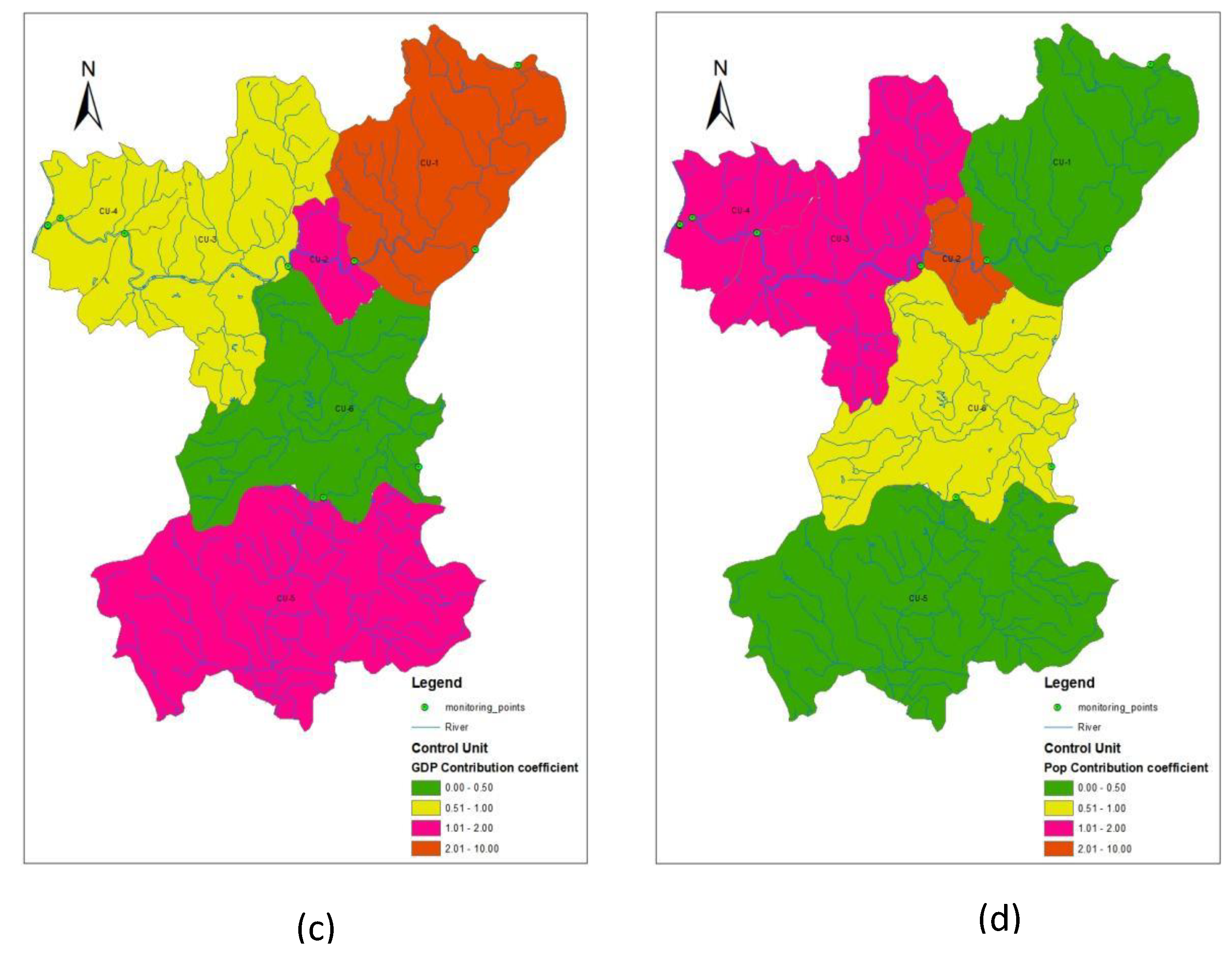
For COD, the contribution coefficients based on the EC values in CU-1, CU-2, CU-3, and CU-6 were less than 1; only CU-3 was greater than 1. The contribution coefficients based on land in CU-1, CU-3, CU-5, and CU-6 were greater than 1, and CU-2 and CU-4 were less than 1. The contribution coefficients based on the GDP in CU-1, CU-3, and CU-6 were greater than 1; CU-2, CU-4, and CU-5 were less than 1. Additionally, the contribution coefficients based on the population in CU-2, CU-3, and CU-5 were greater than 1, and in CU-1, CU-4, and CU-6, they were less than 1.

For AN, the contribution coefficients based on the EC in CU-3 and CU-4 were greater than 1; CU-1, CU-2, CU-5, and CU-6 were less than 1. The contribution coefficients based on land in CU-3, CU-4, CU-5, and CU-6 were greater than 1, and CU-1 and CU-2 were less than 1. The contribution coefficients based on the GDP in CU-1, CU-3, CU-4, and CU-6 were greater than 1; CU-2 and CU-5 were less than 1. Additionally, the contribution coefficients based on the population in CU-2, CU-3, CU-4, and CU-5 were more significant than 1; CU-1 and CU-6 were less than 1.

For TP, the contribution coefficients based on the EC in CU-1. CU-2, CU-3, and CU-6 were greater than 1, and CN-4 and CN-5 were less than 1. The contribution coefficients based on land in CU-1, CU-2, CU-3, and CU-5 were greater than 1, and only CU-4 was less than 1. The contribution coefficients based on the GDP in CU-1, CU-2, CU-3, and CU-6 were greater than 1; CU-2 and CU-5 were less than 1. Additionally, the contribution coefficients based on the population in CU-1, CU-2, CU-3, and CU-6 were greater than 1, and CU-4 and CU-5 were less than 1.

All the areas with the highest contribution coefficients for COD, AN, and TP were mainly concentrated in the pollution control areas and exhibited a green development model. Additionally, some areas presented the lowest contribution coefficients for COD, AN, and TP, the main factor causing inequality. The economic contribution coefficients of some control divisions for each indicator were the lowest, while their land area contribution coefficients were the largest. It can be seen that the unfair factors based on GDP in the area were mainly concentrated in the mountainous and hilly ecological conservation areas. In contrast, the unfair factors based on the land area primarily focused on central urban pollution control areas.

By analyzing the contribution coefficients of different indicators, it was necessary to adjust the region’s industrial structure as soon as possible, improve resource utilization efficiency, reduce pollution emissions, and take the path of sustainable development.

Natural self-purifying capacity is not effectively used in some districts and is overused in others; among other indicators, it is the most inequitable of all factors. The EGC based on the land area would be smaller, and the COD distribution would be more reasonable. Lushui has some old industrial land in the transition period of industrialization and urbanization, which can realize the transformation of industrial structures and reduce industrial pollution to a greater extent. According to the magnitude of the environmental Gini coefficient of each control unit, the inequitable factors of regional development were analyzed from the four indicators presented. This made it possible to complete some measures to increase the environmental capacity, thus increasing the amount of environmental health risk zones in Lushui. In this way, it was possible to interact with overall urban and industrial planning schemes. Additionally, improving the environment and controlling pollution without affecting urban construction and economic development is possible.

Based on the above analysis, for the present situation of pollution sources and water quality in the area where the lower reaches of the Lushui River are located, we focused more on the water quality during the seasons presenting high pollution levels for COD, AN, and TP, and strengthened the pollution reduction and control measures in the urban section of Lushui River. This was performed to improve the prevention, management, and supervision of industrial pollution sources; speed up the construction of sewage pipe networks and improve the quality of sewage pipes and network coverage; strictly investigate enterprise pollution sources; eliminate the occurrence of stealing, mixing, and missing discharge; strengthen the prevention and control of surface pollution; promote ecological and healthy breeding; optimize the industrial structure; conduct the comprehensive management of the water environment; improve the self-purification capacity of water bodies and environmental capacity; strengthen public participation and social supervision; and strictly enforce environmental regulations and strengthen environmental water management. Applying the Gini coefficient allocation method to the allocation of water environmental capacity is still not the optimal method; although, the Gini coefficient calculation results are more equitable. Therefore, subsequent studies should determine a more appropriate allocation method. Additionally, by analyzing the contribution coefficients of different indicators, it was necessary to adjust the industrial structure of the region as soon as possible; therefore, the Gini coefficient method needed to improve the efficiency of resource utilization. This will support the evaluation of pollution emission reductions and promote sustainable development.

This research focused on analyzing water environmental capacity, investigating pollution reduction, and distributing unfair factors for pollution inequity analysis. It provided us with references for water environmental protection and management practices for the Lushui River as well as other areas.

The method used in this study can also be used in the other areas and can use the results as a reference for subsequent research.

5. Conclusions

In order to respond to the national policy of protecting Lushui River, based on the investigation and analysis of the present status of the main rivers and water quality of Lushui River, the water quality and environmental capacity during different periods were simulated using the WASP model. Additionally, the Gini coefficient method was applied to the allocation of discharge permits. Finally, reductions were determined and corresponding pollution control measures were performed to provide a theoretical basis and decision reference for water environmental protection and management schemes for Lushui River. The main conclusions are as follows. Based on the investigation and analysis of the present situation of water pollution and environmental water quality, and in response to the national policy of protecting the Lushui River, we used the environmental Gini coefficient allocation method to allocate the total amount of COD, AN, and TP discharge permits to the Lushui River Basin. Additionally, four indicators were selected: land area, population, GDP, and water environmental capacity. The pollutant emission reduction of each control unit under the current pollution load conditions was analyzed, and the main conclusions are as follows:

(1)

The water environmental capacity was obtained by calibrating the parameters on the WASP model using the trial-and-error method. The COD values were 14,072.94, 17,147.7, and 10,998.18 t/yr for the normal, abundant, and dry seasons, respectively. However, the results for ammonia nitrogen are 469.098, 571.59, and 366.606 t/yr in the normal, wet, and dry seasons, respectively. In addition, total phosphorus was 93.8196, 114.318, and 73.3212 t/yr in the normal, wet, and dry seasons, respectively. The water environmental capacity of AN, TP and COD in most river sections during the dry season was less than that during the normal and abundant seasons. This was mainly due to the abundant precipitation during the rainy season, which resulted in heavier river flow and higher water dilution environmental capacities.

(2)

Based on the environmental Gini coefficient method, four indicators, population, land area, GDP, and water environmental capacity, were selected to represent social, economic, and environmental factors. After optimization, for COD, the EGC based on land area was 0.30, EGC based on population was 0.21, EGC based on water environmental capacity was 0.002, and EGC based on GDP was 0.45. After optimization, the sum of EGC was 0.962. This result shows that each indicator’s Gini coefficient change is insignificant. Therefore, the most significant change in the Gini coefficient is for GDP, which has a higher rate of change than the other indicators.

(3)

The total COD, AND, and TP discharge permit allocation models were constructed to obtain the total allocated discharge permit in the Lushui River Basin. The results show that the total discharge permits allocated for COD, AN, and TP in the Lushui River Basin were 51,483.304, 843.119, and 340.926 tons/year, respectively.

(4)

Based on GIS spatial analysis technology, the distribution of unfair factors that caused pollution inequity were investigated. All the areas with the highest contribution coefficients of COD, AN, and TP were mainly concentrated in the pollution control areas and exhibited a green development model. Additionally, some areas had the lowest contribution coefficients of COD, AN, and TP, the main factor causing inequality.

(5)

Finally, reduction measures were proposed to implement environmental supervision and strengthen environmental water management.

Therefore, the results obtained by applying the EGC method are applicable and reliable and can be effectively used for the water-quality prediction and evaluation of the Lushui River. They can also be used as references for water environmental protection and management decisions for the Lushui River.

Specific results were obtained by applying the Gini coefficient method to account for water environmental capacity and discharge permit allocation. Based on the research, there are still some limitations: the data for point and non-point source pollution values were limited by some difficulties in the data collection; therefore, the subsequent research must be combined with the actual data for an in-depth analysis. Applying the Gini coefficient allocation method to the allocation of water environmental capacity is still not optimal; although, the Gini coefficient calculation results are more equitable. Therefore, subsequent studies should find a more appropriate allocation method.

References

1. Bosi, S.; Seegmuller, T. Optimal cycles and social inequality: What do we learn from the Gini index? Res. Econ. 2006, 60, 35. [Google Scholar] [CrossRef] [Green Version]
2. Lin, W.; Fu, G. Equitable planning and its application in regional water environmental comprehensive improvement planning. Pollut. Control Technol. 1994, 7, 4–8. [Google Scholar]
3. Xiaoya; Zhang, W.; Yan, W.; Yang, C. Hierarchical analysis of the allocation of pollutants in a specific region of Taihu Lake in the distribution of pollutants in the particular region of Taihu Lake. J. China Inst. Water Resour. Hydropower Res. 2011, 9, 155–160. [Google Scholar]
4. Zheng, X.; Xia, T.; Yang, X.; Yuan, T.; Hu, Y. The land Gini coefficient and its application for land use structure analysis in China. PLoS ONE 2013, 8, e76165. [Google Scholar] [CrossRef]
5. Fang, Y. Allocation of Total Water Pollutant Emissions in the Jiulong River Basin Based on Gini Coefficient Method Research. Environ. Sci. Manag. 2012, 37, 30–35. [Google Scholar]
6. Zhang, H.; Xi, B.D.; Gao, R.T.; Jiang, L.; Wang, J.F.; Xu, Q.G. Calculation of Water Environmental Capacity and Upstream Capacity of Baiyangdian Lake Quantity allocation. J. Environ. Eng. Technol. 2012, 2, 313–318. [Google Scholar]
7. Ziting, G.; Tianyi, P.; Wenjin, Z.; Junyao, Y. The optimization model of surface water pollution allocation based on equity and efficiency. Anhui Agric. Sci. 2012, 40, 8255–8257. [Google Scholar]
8. Burn Durn, D.H.; Mcbean, E.A. Optimization modeling of water quality in an uncertain environment. Water Resour. Res. 1985, 21, 934–940. [Google Scholar] [CrossRef]
9. Deng, Y.X.; Zheng, B.H.; Fu, G.; Lei, K.; Li, Z.C. Study the total water pollutant load allocation in the Changjiang (Yangtze River) Estuary and adjacent seawater area. Estuar. Coast. Shelf Sci. 2010, 86, 331–336. [Google Scholar] [CrossRef]
10. Wu, W.J.; Jiang, H.Q.; Duan, Y.; Liu, N.L.; Lu, Y.L.; Zhang, W.; Yu, S. Optimization of water pollution load distribution in control units based on environmental Gini coefficient. China Popul. Resour. Environ. 2017, 27, 8–16. [Google Scholar]
11. Darkwah, K.A.; Nortey, E.N.N.; Lotsi, A. Estimating the Gini coefficient for the log-normal income distribution using the Lorenz curve. Springer Plus 2016, 5, 1196. [Google Scholar] [CrossRef] [Green Version]
12. Aalami, M.T.; Nourani, V.; Fazaeli, H. Developing a surface water resources allocation model under risk conditions with a multi-objective optimization approach. Water Supply 2020, 20, 1167–1177. [Google Scholar] [CrossRef]
13. Jin, J.; Wang, J.X.; Ma, X.Y.; Wang, Y.D.; Li, R.Y. Equality of medical health resource allocation in China based on the Gini coefficient method. Iran. J. Public Health 2015, 44, 445–457. [Google Scholar]
14. Zhang, X.C.; Wang, F.L. Life-cycle carbon emission assessment and permit allocation methods: A multi-region case study of China population construction sector. Ecol. Indic. 2017, 72, 910–920. [Google Scholar] [CrossRef]
15. Tian, G.; Liu, Z.; Liu, H.; Zhang, C. Yongding River Based on Ecological Characteristics of River Environment Domain Integrated Governance and Management. China Water Conserv. 2019, 34, 42–44. [Google Scholar]
16. Shao, Z.; Liu, L.; Wang, T. Main river pollutants in Zhangjiakou’s upper reaches of the Yongding River Source Analysis. Environ. Pollut. Prev. 2020, 42, 204–211. [Google Scholar]
17. Meng, Q.; Wu, B.; Shen, J.; You, Z. Environmental Gini Coefficient in Water Pollution of Suining City Application in Total Quantity Allocation. Sichuan Environ. 2015, 34, 74–77. [Google Scholar]
18. Yang, R. Research on the Allocation of Total Sulfur Dioxide in Shaanxi Province Based on the Environmental Gini Coefficient Method. Ph.D. Thesis, Northwest University, Xi’an, China, 2016. [Google Scholar]
19. Qin, D.; Wei, A.; Lu, S.; Luo, Y.; Liao, Y.; Yi, M.; Song, B. Dongting Lake Area Based on Environmental Gini Coefficient Total Allocation of water pollution. Environ. Sci. Res. 2013, 26, 8–15. [Google Scholar]
20. Meng, X. Applying the Gini Coefficient Method in the Total Allocation of Water Pollutants. Master’s Thesis, Tianjin University, Tianjin, China, 2007. [Google Scholar]
21. Hao, L.; Ling, N. Initial drainage basin emission rights allocation based on environmental Gini coefficient. People’s Yellow River 2014, 36, 56–59. [Google Scholar]
22. Ling, P. Evaluation and Optimization of Equity in Total Water Pollutant Allocation: A Case Study of Chongqing City for Example. Master’s Thesis, Chongqing University, Chongqing, China, 2014. [Google Scholar]
23. Li, Y.; Wei, H. Gini coefficient of resources and environment in Shaanxi Province and degree of ecological realization Analysis. Hunan Agric. Sci. 2010, 32, 51–54. [Google Scholar]
24. Wang, J.; Lu, Y.; Zhou, J.; Li, Y.; Cao, D. China’s Resource and Environmental Gini Based on GDP Coefficient Analysis. Chin. Environ. Sci. 2006, 26, 111–115. [Google Scholar]
25. Zhai, T.; Guo, J.; Ou, M.; Kong, W. Construction Land in Jiangsu Province Based on Gini Coefficient Research on Total Quantity Allocation. China Popul. Resour. Environ. 2015, 25, 84–91. [Google Scholar]
26. Tian, P.; Fang, X.; Wang, F.; Zhu, Y. Based on the minimization model of environmental Gini coefficient Optimization of Total Water Pollutant Allocation: Take the Zhangjiagang Plain Water Network Area as an Example. China Environ. Sci. 2014, 34, 801–809. [Google Scholar]
27. Xie, G.; Peng, Y.; Li, B.; Han, Y.; Cui, Z. TMDL Plan and Comprehensive Treatment of Small Watershed Pollution Research on Theoretical Thinking: Taking the Shandong Section of the East Line of the South to North Water Diversion Project as an Example for Pollution Control. Agric. Mech. Res. 2006, 28, 189–192. [Google Scholar]
28. Ye, C.; Gu, J. Application of the Gini coefficient method in the total allocation of water pollutants. J. Xihua Univ. (Nat. Sci. Ed.) 2010, 29, 87–91. [Google Scholar]
29. Xiao, Z.; Wan, Z.; Meng, L. Resource and Environmental Base of Guangdong Province Based on Ecological Capacity Calculation and Analysis of Ni Coefficient: Discussion with Zhang Yinbo et al. J. Ecol. 2008, 28, 4486–4493. [Google Scholar]
30. Gan, X.; Wang, S.; Zhao, L.; Wang, L.; Tang, X. Analysis of the Gini coefficient of environmental resources in Sichuan Province. Sichuan Environ. 2015, 34, 111–116. [Google Scholar]
31. Hao, S. Optimal Allocation Method and Water Pollution Load Tracing Application in Plain River Network Area. Master’s Thesis, University of the Chinese Academy of Sciences, Beijing, China, 2016. [Google Scholar]
32. He, W.; Liu, D.; Wang, C. Are Chinese provincial carbon emissions allowances misallocated over 2000–2017? Evidence from an extended Gini-coefficient approach. Sustain. Prod. Consum. 2022, 29, 564–573. [Google Scholar] [CrossRef]
33. Hu, Z.; Chen, Y.; Yao, L.; Wei, C.; Li, C. Optimal allocation of regional water resources: From a perspective of equity-efficiency tradeoff. Resour. Conserv. Recycl. 2016, 109, 102–113. [Google Scholar] [CrossRef]
34. Jiang, H.Q.; Shao, X.; Zhang, X.; Bao, J. A study of the allocation of carbon emission permits among the provinces of China based on fairness and efficiency. Sustainability 2017, 9, 2122. [Google Scholar] [CrossRef] [Green Version]
35. Li, A.; Yuan, Q.; Strokal, M.; Kroeze, C.; Ma, L.; Liu, Y. Equality in river pollution control in China. Sci. Total Environ. 2021, 777, 146105. [Google Scholar] [CrossRef]
36. Wu, W.; Jiang, H.Q. The control unit’s total water pollutant load distribution application is based on the environmental Gini coefficient. China Popul. Resour. Environ. 2017, 5, 8–16. (In Chinese) [Google Scholar]
37. Zhou, S.; Du, A.; Bai, M. Applying the environmental Gini coefficient in allocating water governance responsibilities: A Taihu Lake Basin, China case study. Water Sci. Technol. 2015, 71, 1047–1055. [Google Scholar] [CrossRef]
38. Zhang, B.; Liu, H.; Yu, Q.; Bi, J. Equity-based optimization of regional water pollutant discharge amount allocation: A case study in the Tai Lake Basin. J. Environ. Plan. Manag. 2012, 55, 885–900. [Google Scholar] [CrossRef]
Figure 1. Overview of the study area.
Water 15 02156 g001
Figure 2. EGC calculation using the Lorenz curve.
Water 15 02156 g002
Figure 3. Wastewater discharge management structure in China.
Water 15 02156 g003
Figure 4. Environmental Gini method flowchart.
Water 15 02156 g004
Figure 5. (ac) Distribution of COD, AN, and TP discharge permits in each control unit after optimization.
Water 15 02156 g005
Figure 6. (ac) Lorenz curve of COD, AN, and TP discharge permits based on land area after optimization.
Water 15 02156 g006
Figure 7. (ad) Distribution of COD contribution coefficients in Lushui River based on the four indicators.
Water 15 02156 g007aWater 15 02156 g007b
Figure 8. (ad) Distribution of AN contribution coefficients in Lushui River based on the four indicators.
Water 15 02156 g008aWater 15 02156 g008b
Figure 9. (ad) Distribution of TP contribution coefficients in Lushui River based on the four indicators.
Water 15 02156 g009aWater 15 02156 g009b