Modelling and Numerical Simulation Approaches to the Stage–Discharge Relationships of the Lansheng Bridge

Abstract

In recent years, extreme rainfall events with short delays and heavy rainfall have often occurred due to severe climate change. In 2015, Typhoon Soudelor caused a short-delayed heavy rainfall event in Nanshih River, which caused damage to a section of the Lansheng Bridge discharge station. The section was relocated upstream to rebuild the discharge station in 2019. However, the new discharge station cannot measure high flow due to the bridge structure. The flow observation range of Lansheng Bridge is therefore limited to normal flow, making it impossible to accurately estimate the flow during high-water stages. The purpose of this study is to use the past flow data of Nanshih River to estimate the flow rate under different return periods using frequency analysis. We used a Digital Elevation Model (DEM) to map the river’s topography, and used the 3D hydraulic calculations of the FLOW-3D model to estimate the water stage and discharge of the Lansheng Bridge. We then verified the accuracy of the model with the measured flow and water stage, and finally used the water stage and discharge data obtained from numerical simulation to construct the stage–discharge rating curve of the Lansheng Bridge. In addition to preventing flood disasters, this study approach can provide reliable data for use in water conservation. It may also be utilized to overcome the problem of measuring and estimating high flow during typhoon floods.

1. Introduction

Nanshih River is one of the critical water sources in Taipei, and it is the main river of the Greater Taipei Flood Control System. Therefore, in the past, a lot of workforce and material resources were invested in the construction of the stage–discharge rating curve of the Lansheng Bridge at Nanshih River for water resource management, flood control calculations, and hydraulic engineering. Chen [1] proposed an effective flood measurement method for mountainous rivers at the Lansheng bridge, considering personal safety, accuracy, and reliability. The proposed method utilizes a torrent measurement system consisting of an acoustic Doppler profiler and a crane system to measure velocity distribution, cross-sectional area, and water depth, and to establish the relationship between mean and maximum velocity and between cross-sectional area and elevation. Once the method is established, the flood flow of the Nanshih River can be estimated effectively using the maximum velocity and water level. In August 2015, Typhoon Soudelor swept across Taiwan. After Typhoon Soudelor, a section of the Lansheng Bridge discharge station was severely silted up, which made it impossible to accurately estimate the discharge from the past rating curve [2]. Therefore, the discharge station was moved to a new bridge (the river system was not impacted, since the new bridge lacks piers), so the stage–discharge rating curve needed to be re-established. To establish the stage–discharge rating curve for high flow, it was necessary to accurately measure high flow values. However, measuring high flow during typhoon floods is difficult, time-consuming, labor-intensive, and dangerous. Using numerical hydraulic models to simulate different water stages to obtain high discharges and establish a stage–discharge rating curve is one way to solve the dilemma mentioned above.

The stage–discharge rating curve is mainly established based on normal discharge and water stage measurements, and by collecting enough data to develop the relationship between water stage and discharge [3]. Owing to the high flood velocities, flood discharge usually cannot be measured. Therefore, some hydraulic and hydrological models are used to establish the relation of stage and discharge in rivers. In the case of significant uncertainties, the stage–discharge rating curve can also be constructed using dimensional analysis [4]. In addition, numerical simulation can also be applied to establish the stage–discharge relationship. The numerical hydraulic model is a method for calculating water stage, water depth, and flow velocity according to different water flow characteristics. It uses physical theory, numerical methods, and grid calculation in its simulations. Three significant elements make up a numerical hydraulic model: governing equations, numerical discretization, and input conditions. Whether they are one-dimensional [5,6], two-dimensional [7,8], or three-dimensional hydraulic models [9,10], the governing equations are fundamental to determine the flow characteristics of water bodies. The governing equations used in basic hydraulics are those of the conservation of continuity, momentum, and energy. In the face of continuous numerical data of the flow field, it is necessary to discretize it to reduce the complexity of the calculation while ensuring the step size and quality of the analysis [11]; the actual flow field conditions should be used to input the various parameters so that the simulation result is closer to the real situation.

Numerical hydraulic analysis selects the most suitable calculation method according to channel characteristics and local river sections. The calculation of the three-dimensional hydraulic model is quite complicated, but it is also relatively accurate [12]. In addition to the vertical and horizontal flow, the three-dimensional hydraulic model also considers vertical flow. Due to the huge calculation time, the 3D hydraulic model is usually used in small areas. It is also often analyzed in areas with apparent vertical flow, such as density current flow, water conservancy facilities, and bridge pier scour [13]. Hu et al. [14] evaluated the applicability of flow models with different spatial dimensions in hydraulic characterization solutions with parameters such as free liquid surface, water depth variation, and average velocity in dam breaks under wet and dry conditions, among others. He studied two similar 3D hydrodynamic models (FLOW-3D and MIKE 3 FM) in dam failure simulations and compared the results with experimental data and 1D analytical solutions. The study results show that the FLOW-3D model better captures the wavefront free surface profile of both dry and wet beds.

The Lansheng Bridge is located near a confluence of rivers, and the downstream is easily affected by the backwater of the Guishan Dam, which complicates the flow conditions there. Therefore, to understand the influence of the flow field near the Lansheng Bridge on the discharge station, the relationship between discharge and water stage was constructed using a complex 3D hydraulic model. This study uses Nanshih River’s annual maximum flow series data (2005–2015) and the frequency analysis method (Pearson Type III) to estimate the flood peak flow of Nanshih River’s 2-year, 10-year, 100-year, and 200-year return periods. The critical water depth relationship generated when the downstream Guishan Dam is released was used as the boundary condition. The grid Digital Elevation Model data was used to construct the river channel topography. Then, the three-dimensional hydraulic calculation method of the FLOW-3D model calculates the peak flood water level under different return periods. Based on this, the stage–discharge rating curve of high discharge from Lansheng Bridge was drawn using the stage–discharge relationship of different return periods. This solves the problem of insufficient high-discharge data after the Lansheng Bridge was broken. The flowchart of these studies is shown in Figure 1. This research method can also solve the difficulty of measuring high flow during typhoon floods and provide credible application data for water conservation and to prevent flood disasters.

2. Study Area

As shown in Figure 2, the Lansheng Bridge discharge station is located on the Nanshih River in northern Taiwan, about 350 m upstream of the Nanshih River and Tonghou River confluence. Nanshih River is the primary tap water source in the greater Taipei area, with a total length of 45 km and a drainage area of 332 square kilometers. Tonghou River, Nanshih River’s most major tributary, also flows into Nanshih River downstream of Lansheng Bridge. In the study area, the high temperature in summer is 30 °C~33 °C, the low temperature in summer is 24 °C~25 °C, the high temperature in winter is 18 °C~23 °C, and the low temperature in winter is 13 °C~18 °C. Affected by the northeast monsoon in winter, it is humid and rainy; in summer, the southwest monsoon is blocked by mountains and has little impact on the Nanshih River area, but the convection effect caused by solar radiation is strong in summer, and heavy rainfall often occurs in the afternoon. In addition, in summer and autumn, typhoons will bring a lot of rainfall. The annual rainfall is between 3000 and 5000 mm. The scope of 3D hydraulic calculation in this study covers the Nanshih River and Tonghou River near the Lansheng Bridge. The upstream boundary starts at 300 m upstream of the Lansheng Bridge of the Nanshih River and 500 m upstream of the Wulai Bridge of the Tonghou River, and the downstream boundary ends at Guishan Dam, about 1.34 km in length.

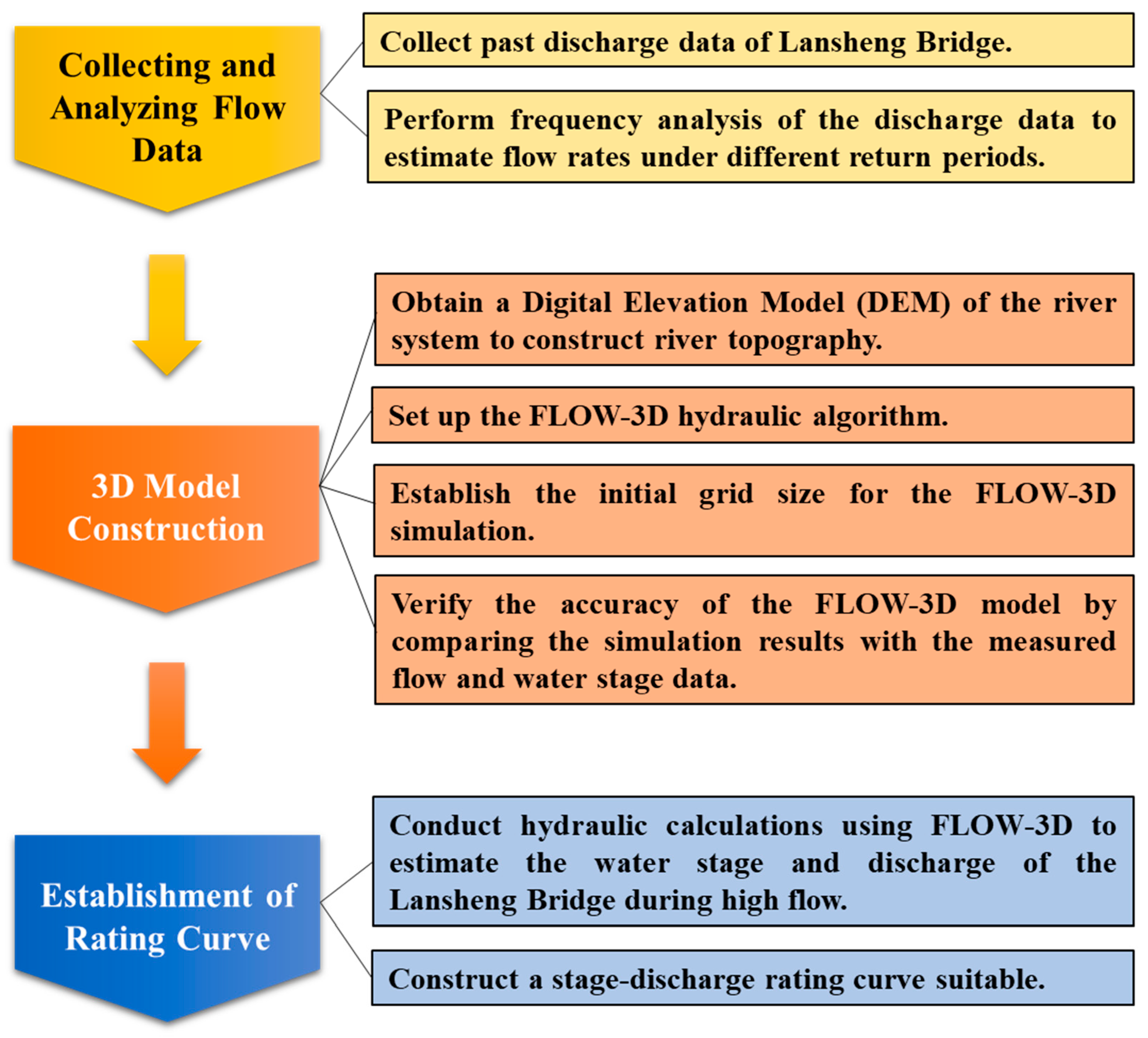
3. Three-Dimensional Hydraulic Calculation

3.1. FLOW-3D

FLOW-3D is a Computational Fluid Dynamics (CFD) software developed by Hirt in 1985. Users can construct various physical models and apply them in different engineering fields according to their needs [15,16]. CFD mainly discretizes and solves through the fluid governing equations (conservation of mass, momentum, and energy). This method comprises the numerical solution of a specific governing equation given initial and boundary conditions. FLOW-3D can also operate in different fluid situations, for example, compressible or incompressible flow calculation. In addition, there may be one or two fluid modes for the user to choose from.

The Volume of Fluid Method (VOFM) [17] is now widely used in computational fluid dynamics to deal with problems with different fluid interfaces. Since the VOFM discriminates the flow situation by processing the momentum equation and calculating the fluid fraction through the control volume, it can be used for flows with free liquid surfaces or fluid stratification. According to the definition of the Volume of Fluid function, F(x, y, z, t) means that the fluid per unit volume satisfies the following formula:

$$\frac{\partial F}{\partial t}+\frac{1}{V_F}\left[\frac{\partial }{\partial x}\left(F{A}_{x}u\right)+R\frac{\partial }{\partial y}\left(F{A}_{y}v\right)+\frac{\partial }{\partial z}\left(F{A}_{z}w\right)+\xi \frac{F{A}_{x}u}{x}\right]=F_{DIF}+F_{SOR}$$

(1)

$F_{DIF}$ is:

$$F_{DIF}=\frac{1}{V_F}\left\{\frac{\partial }{\partial x}\left({\nu }_F{A}_x\frac{\partial F}{\partial x}\right)+R\frac{\partial }{\partial x}\left({\nu }_F{A}_{y}R\frac{\partial F}{\partial y}\right)+\frac{\partial }{\partial z}\left({\nu }_F{A}_z\frac{\partial F}{\partial z}\right)+\xi \frac{{\nu }_F{A}_{x}F}{x}\right\}$$

(2)

where V_F is the fractional volume; u, v, and w are the flow velocities in x, y, and z directions, respectively; A_x, A_y, and A_z are the fractional areas in x, y, and z directions, respectively; R and $\xi$ are the coordinate conversion coefficients. v_F is the diffusion coefficient, v_F = cFμ/ρ, where μ is the dynamic viscosity, ρ is the fluid density, and cF is a constant whose reciprocal is called the Schmidt number. F_DIF is a fluid fraction diffusion term; F_SOR is a fluid volume mass source term.

The function F is used to explain the state of the fluid at different volume fractions, whether it is full of liquid, has a free liquid surface, or is full of air. For a single fluid, function F represents the volume fraction of the fluid [18]. When F = 1, it means that the fluid is full of volume; when 0 < F < 1, it means a free liquid surface is present in the volume; when F = 0, it means that the volume is filled with air.

FLOW-3D uses the Finite Difference Method (FDM) to construct the discretization process of numerical equations [19]. The principle of FDM is to approximate partial differential equations with difference equations, divide the area to be solved into finite grids, and use initial conditions, boundary conditions, and recursive formulas to find the values of all nodes in the grid. FDM converts nonlinear ordinary or partial differential equations into a linear equation that can be solved through matrix algebra. FDM will appear more challenging when faced with complex geometric boundaries. In addition, the value calculated by FDM needs to rely on the nodes between the grids, so this method must use a structured grid.

FLOW-3D has the advantage of faster calculation speed when using structured grids than unstructured grids [20]. However, in the face of complex geometric shapes, structured grids must describe difficult parts of the model by increasing the number of grids. To describe the physical model of the single-block-structured grid traditionally used in building structured grids, it is often necessary to build a large number of grids. If the model is more complex, the areas outside the model often waste calculation and increase the calculation time. The multi-block-structured grid can solve the above problems and refine and calculate the complex flow area for the local grid.

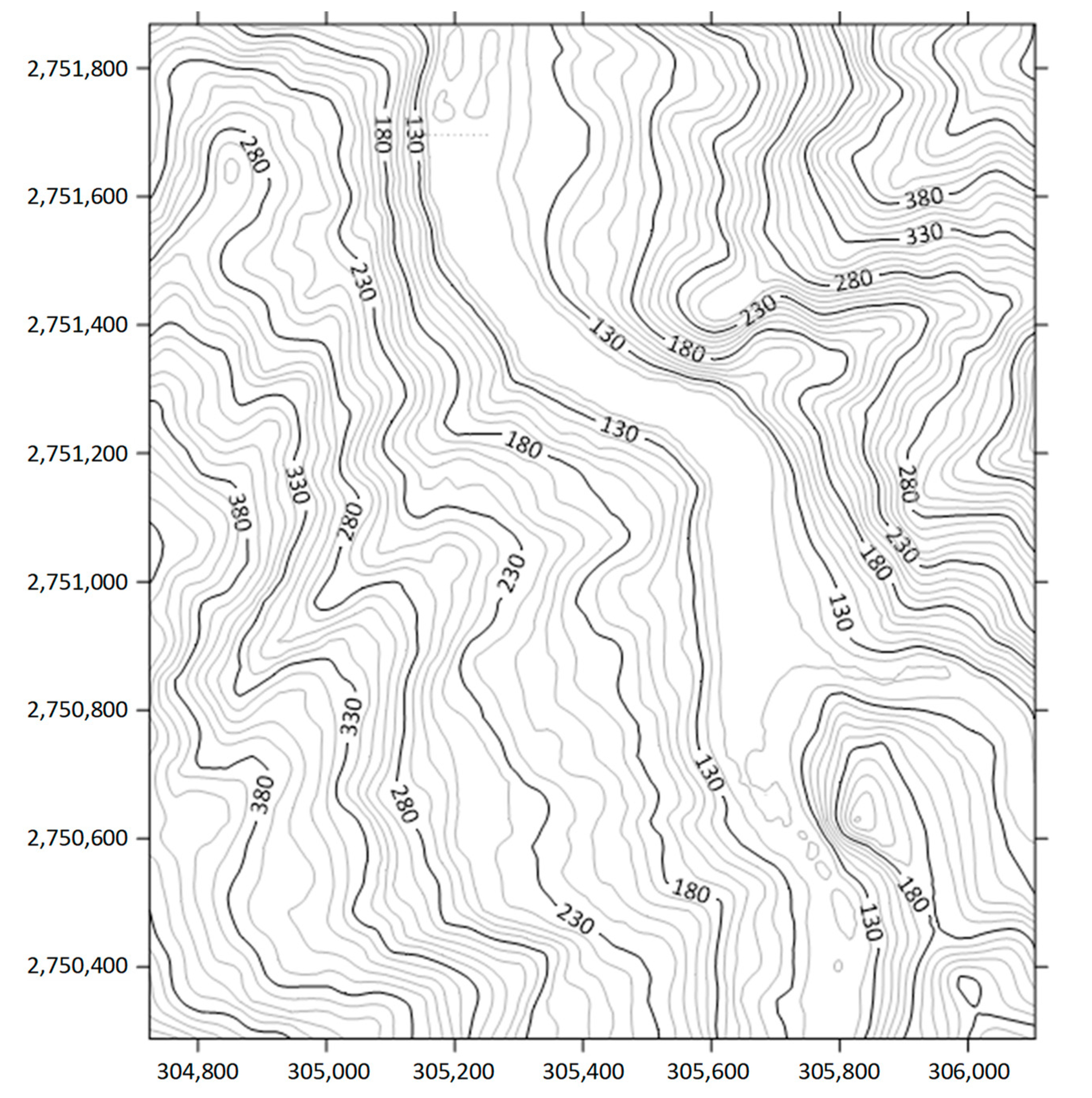
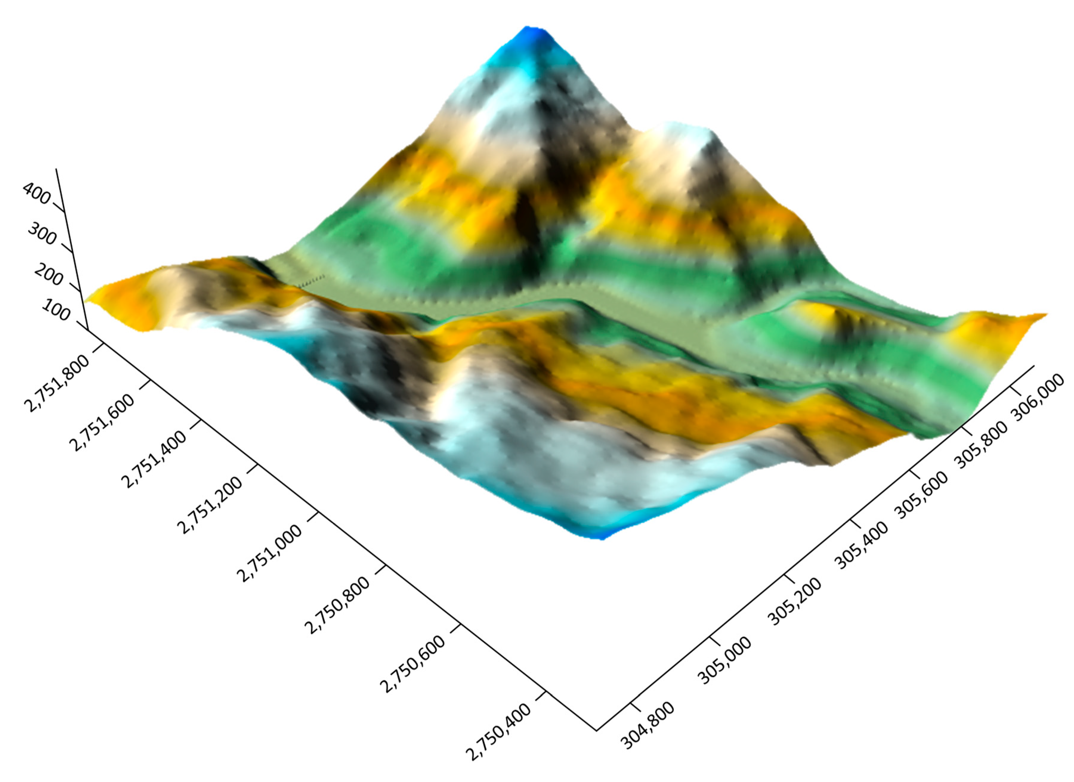
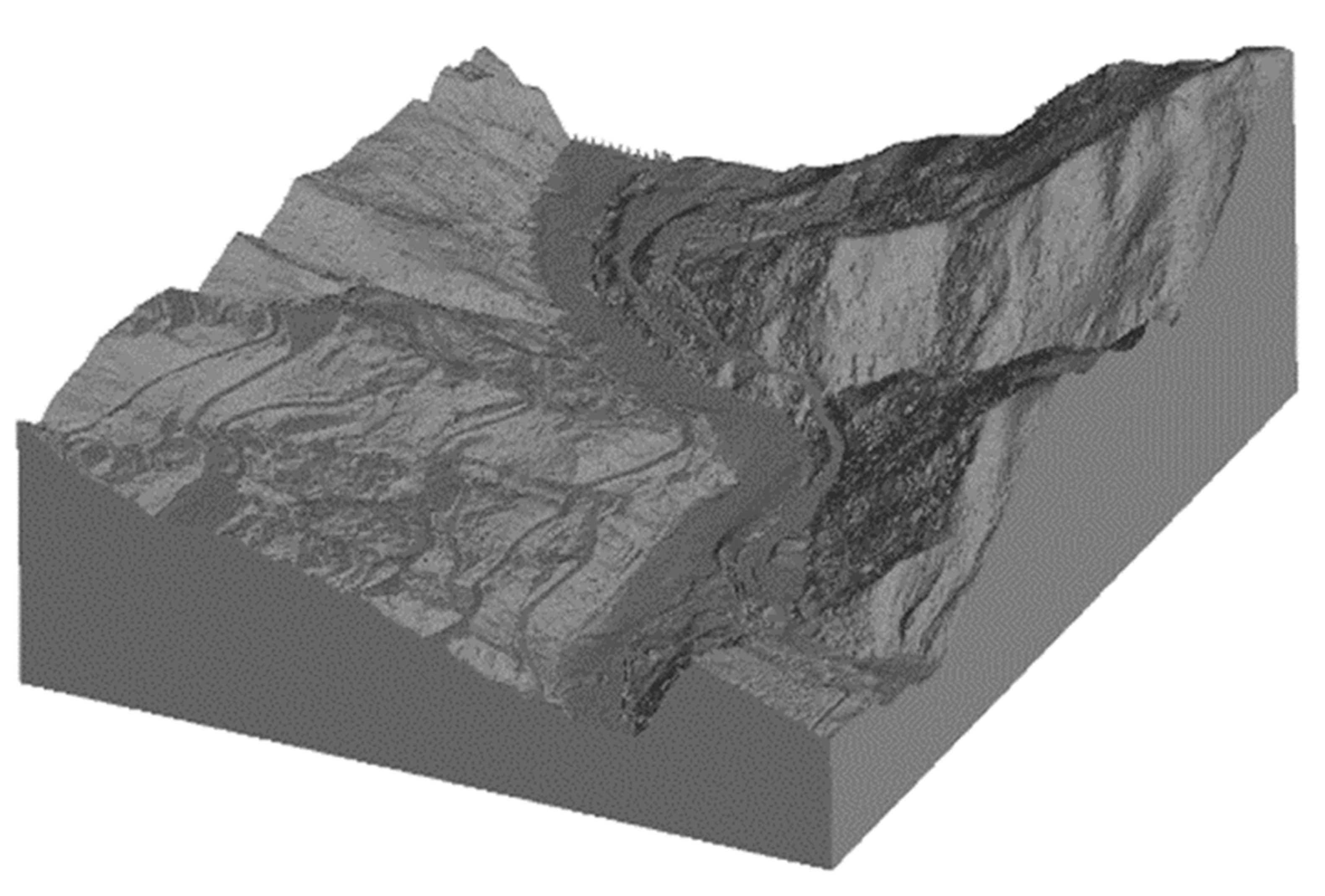
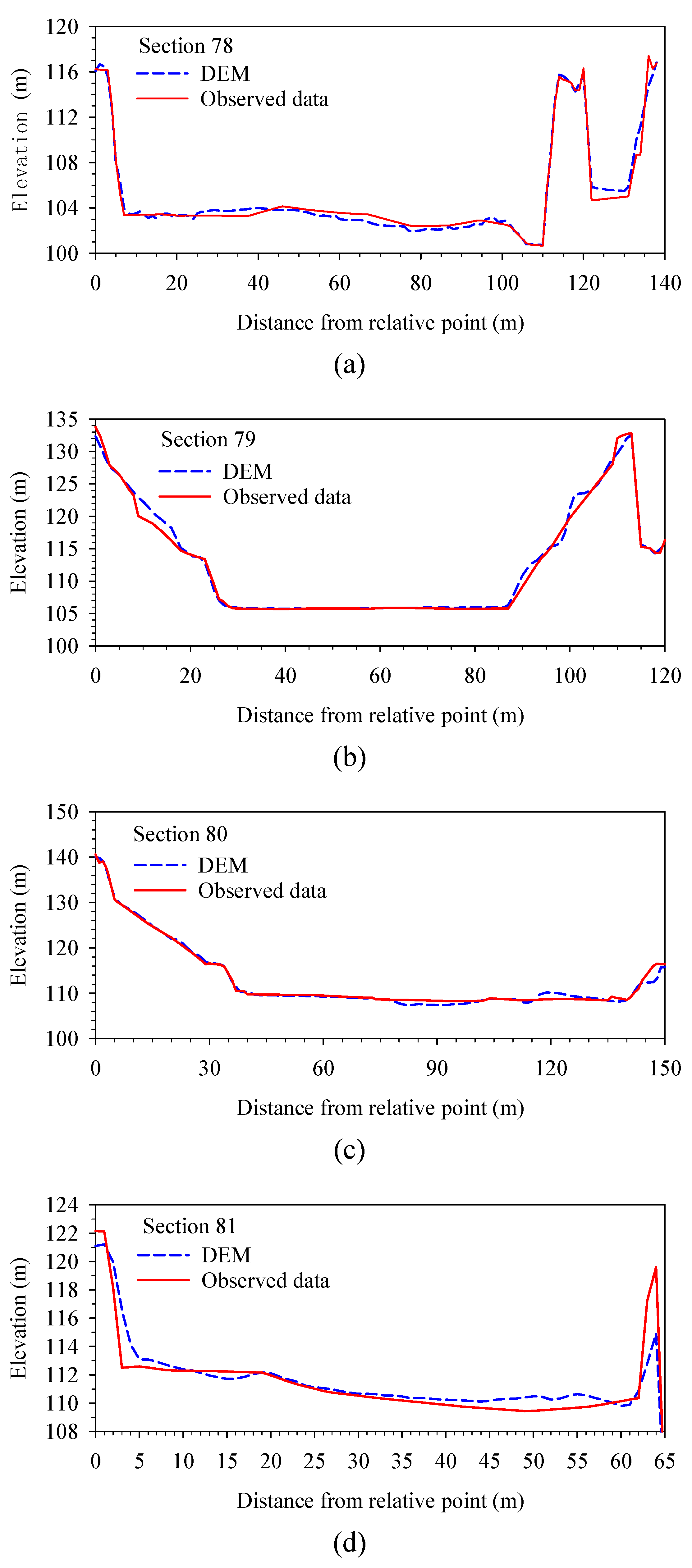
3.2. River Topography Data

Traditionally, the measurement of river channel topography is usually obtained through large-scale cross-section measurement. However, the discharge station of Lansheng Bridge is located upstream of the catchment area, and there is no need for flood control, so large-scale cross-section measurement has yet to be carried out. Therefore, this study uses the 2015 DEM [2] to construct the river topography of the Nanshih River and Tonghou River. Airborne LiDAR can efficiently acquire wide-area, high-density, and high-resolution DEM data [21], and was used to measure the DEM of this study area. Its resolution is 1 m × 1 m. This study uses the 3D analysis function of geographic information system (ArcGIS) to analyze the cross-sectional data of the DEM to obtain the topography of the river.

3.3. Frequency Analysis for Determining the Discharges

This study used the discharge measured by the Lansheng Bridge in the Nanshih River section before the station was relocated to estimate the range of the rating curve discharge. We used the Pearson type III distribution to estimate the frequency factor (K_T), then calculated the peak flood discharge under different return periods according to Formula (3):

$$x_T=\mu +\sigma K_T$$

(3)

where x_T is the hydrological volume of return period T; μ is the average value of hydrological data; σ is the standard deviation of hydrological data; and K_T is frequency factor.

After using frequency analysis to obtain the discharges in different return periods, this study used the chi-square test to determine the fit between the observed results and the expected results and to confirm whether the Pearson Type III distribution could reasonably be used to estimate the discharges in different return periods.

3.4. Establishment of 3D Model

The scope of the 3D simulation in this study was the confluence area of the Nanshih River and Tonghou River. After obtaining the DEM grid file of the terrain data, the Surfer software (the version number is 12) was used to convert the grid into contour lines (including Z values). Then, the terrain uplift function was used to output it into STL format (FLOW-3D default format). After importing the model file to FLOW-3D, the model parameters can be set. This study used the Surfer software modeling tool to obtain the contour map (Figure 3) and then output the contour line into a three-dimensional surface map (Figure 4). Finally, we filled the bottom and four sides of the three-dimensional surface graph into solids, and exported it as an STL file (as shown in Figure 5). The coordinate system used in Figure 3 and Figure 4 is the World Geodetic System 1984 (WGS84), a standard created by the United States National Geospatial Intelligence Agency for cartography, geodesy, and satellite navigation.

Table 1. Block grid construction range (meters).

		X	Y	Z
Block 1	Min	305,122	2,751,400	90
	Max	305,382	2,751,694	130
Block 2	Min	305,482	2,750,620	90
	Max	305,792	2,750,770	130
Block 3	Min	305,782	2,750,760	90
	Max	305,972	2,751,200	130
Block 4	Min	305,482	2,750,760	90
	Max	305,792	2,751,210	130
Block 5	Min	305,122	2,751,200	90
	Max	305,382	2,751,410	130
Block 6	Min	305,372	2,751,200	90
	Max	305,492	2,751,410	130
Block 7	Min	305,482	2,751,200	90
	Max	305,792	2,751,410	130
Block 8	Min	305,482	2,750,590	90
	Max	305,882	2,750,750	130
Block 9	Min	305,962	2,750,430	90
	Max	306,182	2,750,960	130
Block 10	Min	306,172	2,750,430	90
	Max	306,332	2,750,600	130

shows the location of grid blocks that were established in this study, and the construction range is shown in Figure 6. The grid blocks indirectly have overlapping areas for program calculations. Grid construction set the range of x, y, and z according to the coordinate origin. The grids were set in the water flow simulation area to avoid wasteful calculations.

The model’s boundary conditions used the input of different types of boundary conditions for the six sides, so that the program can identify the watershed conditions. In this mode, the Y_min (Nanshih River) of Block 2 was set as the inflow boundary condition; the X_max (Tonghou River) of Block 3 was set as the inflow boundary condition; the Y_max of Block 1 was set as the outflow boundary condition; and the other contour surfaces were selected as the wall boundary conditions. The overlap between blocks was set as the overlapping boundary condition; the Z_max of each block was set as the symmetrical boundary condition; Z_min was set as the wall boundary condition.

The roughness coefficient used in the FLOW-3D program is not Manning’s Roughness Coefficient, as is used in general open channel flow, but rather the roughness height is used as the model surface roughness (k). The model surface roughness can be estimated by using Manning’s Roughness Coefficient and Formula (4) [22].

$$k={\left(\frac{n}{0.0389}\right)}^6$$

(4)

where n is Manning’s Roughness Coefficient.

The 10th River Management Office investigated the river bed sediment in this study area in 2007, and Manning’s Roughness Coefficient of the river section was calculated to be 0.042 [23]. After conversion by Formula (4), k was found to be obtained 1.5842.

4. Simulation Results

4.1. Creation of River Topography

Within the range of the study, four large sections were measured in 2015 [23]. Their locations are shown in Figure 2, and the section numbers are Section 78, Section 79, Section 80, and Section 81. Figure 7 compares the section analyzed by DEM and measured in 2015. After calculating the root mean square error (RMSE), it can be seen that the RMSEs of Section 78, Section 79, Section 80, and Section 81 are 0.14 m, 0.38 m, 0.25 m, and 0.29 m, respectively. This shows that the error of the simulation analysis results is not significant, so the high-resolution DEM can be used to construct the river topography required by the model, and the use of DEM for hydraulic analysis can save a lot of time, labor, and material resources in the measurement of river topography.

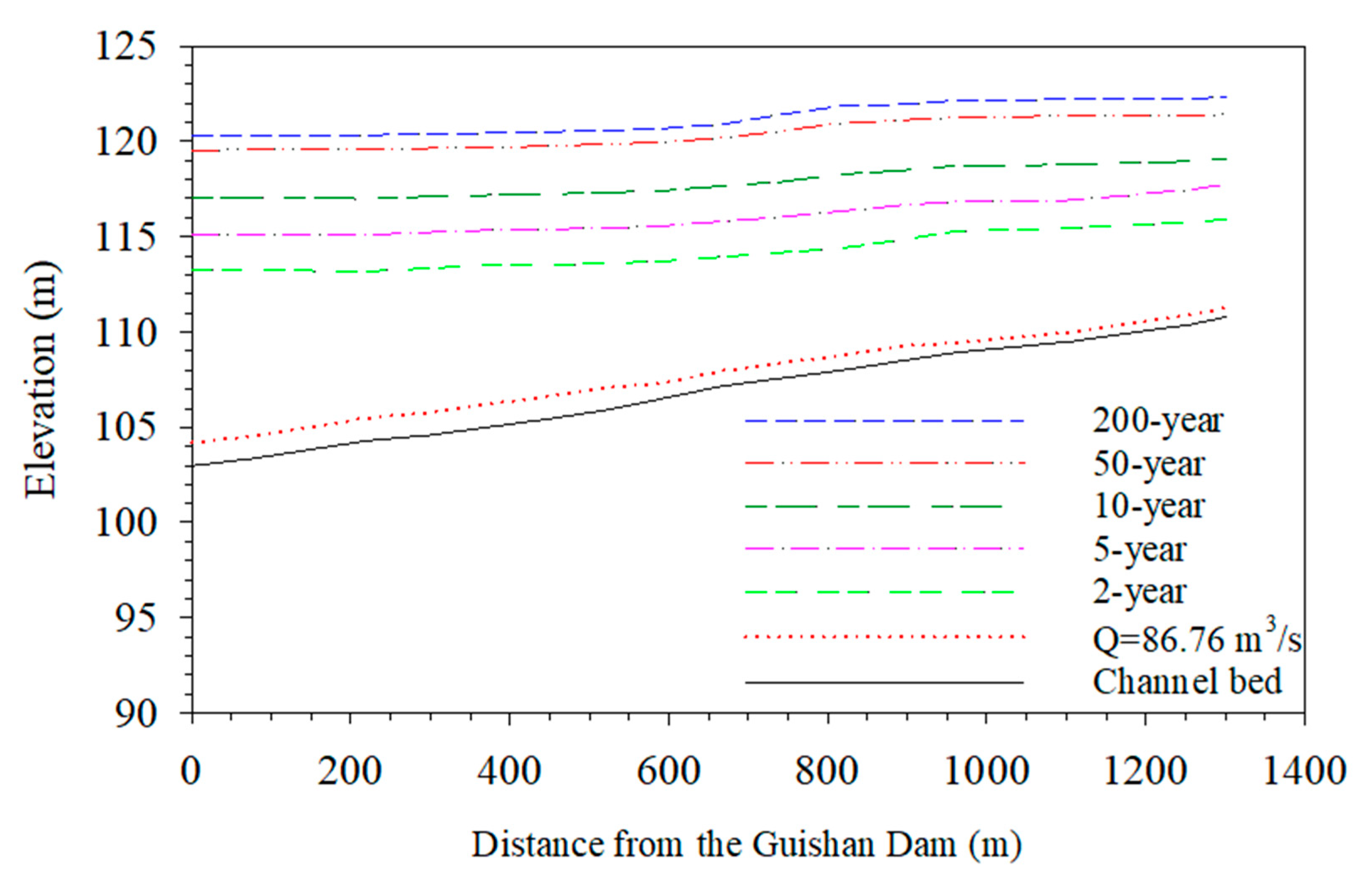
4.2. Estimation of Discharges in Different Return Periods

The Lansheng Bridge discharge was recorded from 2005 to 2015, with 11 years of discharge data.

Table 2. Annual maximum discharge of the Lansheng Bridge.

Year	2005	2006	2007	2008	2009	2010	2011	2012	2013	2014	2015
Discharge (m3/s)	2094	1712	1867	1169	617	624	375	1559	601	503	2255

shows the annual maximum discharge of Lansheng Bridge from 2005 to 2015.

Table 3. Estimated the flood discharges of Nanshih River and Tonghou River with different return periods using Pearson Type III.

Return Period (Year)		2	5	10	15	25	50	100	150	200
Discharge (m3/s)	Nanshih River	1166	1788	2143	2327	2544	2816	3070	3212	3310
	Tonghou River	437	671	804	873	954	1056	1151	1205	1241

shows the frequency analysis results of each return period of the Lansheng Bridge. The χ² test was conducted to determine whether the Pearson Type III distribution adequately fitted the data. The χ² test statistic is ${\chi }_{2,c}^2$ = 0.369, and the value of ${\chi }_{2,0.95}^2$ is 3.841. Because ${\chi }_{2,0.95}^2$ > ${\chi }_{2,c}^2$, these discharges can be said to fit the Pearson Type III distribution. The results indicate that the proposed method can be used to reliably estimate the return period discharges.

There is no required discharge data for the Tonghou River, so the discharge of the Lansheng Bridge was used with the area ratio method to estimate it [24]. The area ratio method formula is Q₁/Q₂ = (A₁/A₂)^m, where m is an undetermined coefficient. Since the catchment area of the Nanshih River is close to the catchment area of the Tonghou River, the geographical location is similar, the hydrology and geology conditions between the two catchment areas are very similar, and the soil type is the same (young yellow soil). Therefore, the undetermined coefficient (m) was assumed to be 1 in this study. The catchment area of Lansheng Bridge is 224.74 square kilometers, and the catchment area of Wulai Bridge is 84.19 square kilometers. So Q₁/Q₂ = (A₁/A₂)^m = (84.19/224.74)¹ = 0.375. Table 3 also shows the estimated return period flows of the Tonghou River based on the area ratio.

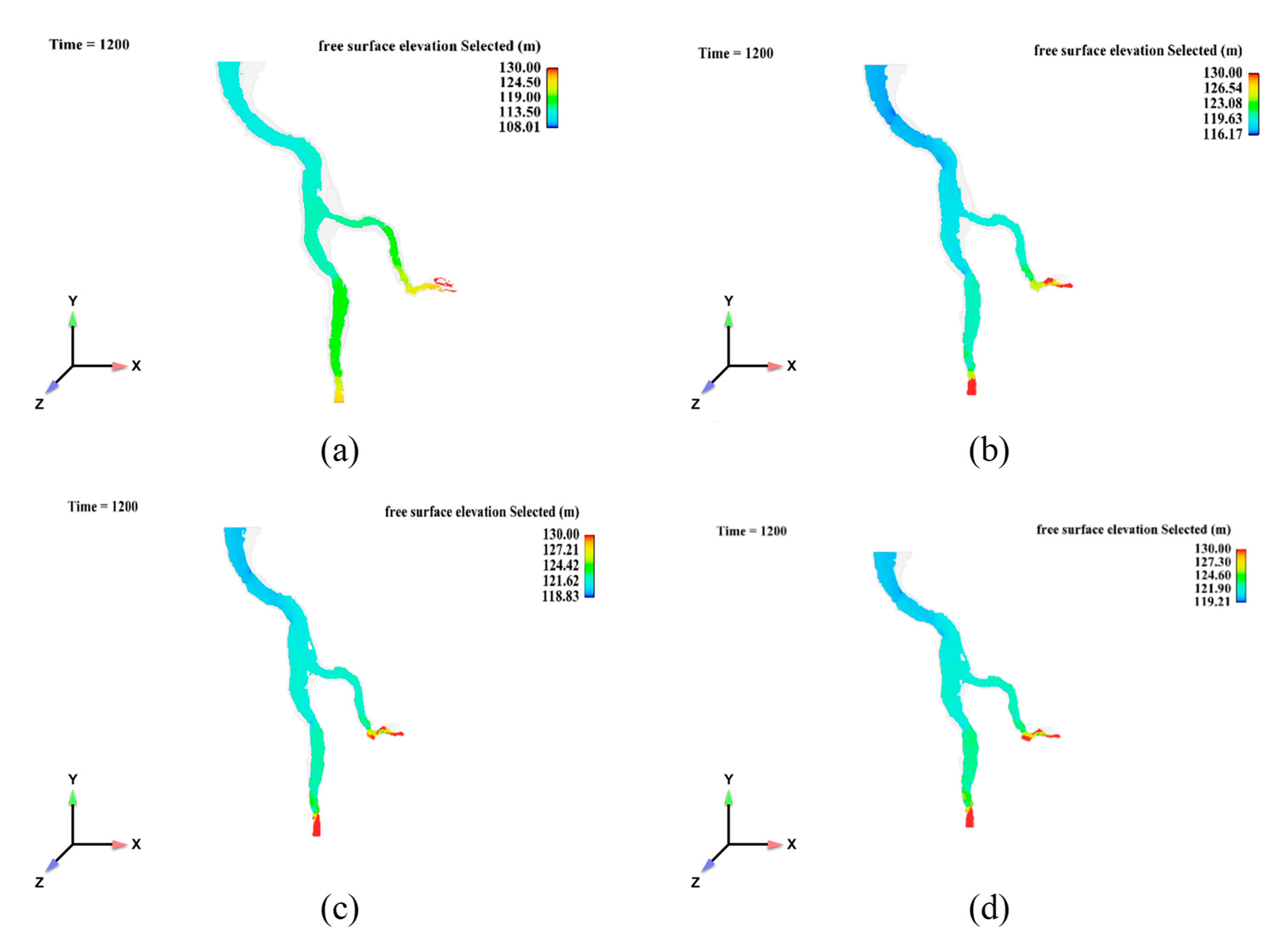
4.3. Estimate Water Level with FLOW-3D

To construct a feasible FLOW-3D model, this study uses the measured discharge of Lansheng Bridge in recent years to verify the reliability and accuracy of the model. If the water stage obtained from the normal discharge analysis qualified, the FLOW-3D hydraulic analysis method was considered to be feasible in this study area. The process of simulating with FLOW-3D includes importing required data for simulation, model setting, defining simulation grid size, boundary condition setting, fluid setting, output item setting, and simulation result analysis. Based on this process, the simulation analysis results of the water level estimated with FLOW-3D are described below.

The interval for normal discharge measurement is once every two weeks, and the opportunity for high flow measurement will be increased according to the discharge situation to maximize the range of water level and discharge curve measurement. In this study, five pieces of discharge data from the flow measured after the Lansheng Bridge moved to the new station, from smaller to larger (as shown in

Table 4. Simulation results of normal discharge.

Date	Observed Discharge (m3/s)	Observed Elevation (m)	Estimated Elevation (m)	Error (m)
6 January 2022	15.11	109.82	109.78	−0.04
10 February 2022	19.22	109.91	109.85	−0.06
9 June 2022	22.65	110.02	110.15	+0.13
5 August 2021	86.76	110.40	110.36	−0.04
18 August 2021	67.49	110.18	110.21	+0.03

), were selected as the input conditions of the upstream boundary of the model to simulate the real flow occurrence. The upstream boundary of the normal discharge simulation range in this study is 300 m upstream of the Lansheng Bridge of the Nanshih River and 300 m upstream of the Wulai Bridge of the Tonghou River, and the downstream boundary ends at Guishan Dam of the Nanshih River. The grid settings were all 0.1 m. Due to the low water depth under normal discharge, if a grid with a larger scale of more than 1 m is used, the simulation may not be carried out smoothly, or the simulation effect may not be good. The results of normal discharge simulation using FLOW-3D in this study are also shown in Table 4. From Table 4, it can be seen that the difference between the water level simulated by the model and the measured water level is between −0.04 m and +0.13 m, and the error is very small. The Nash–Sutcliffe Efficiency (NSE) coefficient in Formula (5) can be used as a criterion to verify whether the hydraulic model is good or bad.

$$NSE=1-\frac{{{\displaystyle \sum }}_{t=1}^T{\left(Q_o^t-Q_m^t\right)}^2}{{{\displaystyle \sum }}_{t=1}^T{\left(Q_o^t-\overline{Q_o}\right)}^2}$$

(5)

In the Formula (5), $Q_o$ is the observed value; $Q_m$ is the simulated value; $Q^t$ is the hydrological value at time t; and $\overline{Q_o}$ is the total average of the observed values.

Generally, when the NSE is more significant than 0.75, it is judged that the model quality is good [25]. The NSE of this study’s normal discharge simulation results is 0.79, which shows that FLOW-3D can accurately simulate the flow and water level during normal times. Figure 8 shows the relationship between the normal discharge and the water stage of Lansheng Bridge. The circle is the measured flow, and the triangle is the relationship between flow and water level simulated by FLOW-3D. All the triangles fall near the circle, which shows the reliability of the model simulation with accuracy. This result also indicates that it is feasible to use FLOW-3D to conduct a three-dimensional hydraulic analysis in the Nanshih River basin.

Finally, the discharges calculated in this study with different return periods were brought into FLOW-3D for simulation. We conducted a hydraulic analysis of the discharge with return periods of 2 years, 10 years, 100 years, and 200 years to estimate the stage of Lansheng Bridge. Then, we utilized the discharge and stage of different return periods to establish a high discharge rating curve suitable for Lansheng Bridge. This simulation adopted quantitative flow and ran for 1200 s. To ensure that the steady state may be obtained under different discharges, the computation finished when the steady state is reached. Figure 9 illustrates the estimated water stages in the modeled area under different return periods. Figure 10 details the water stage profile of Nanshih River under the normal discharge and the discharge of different return periods. It can be seen from Figure 10 that the water stage difference between upstream and downstream is significant at a normal discharge, whereas the water stage drop difference is small at a high discharge.

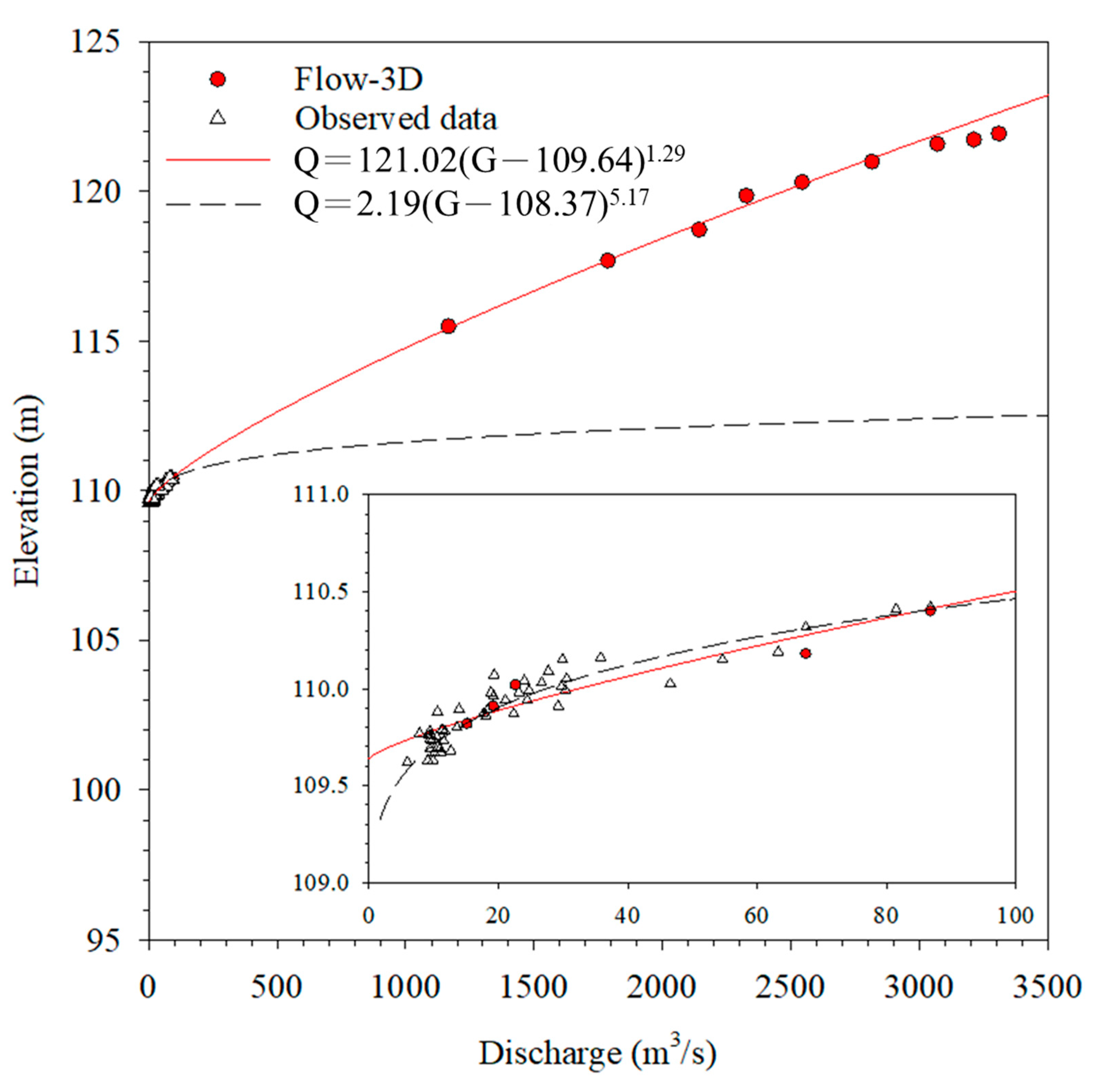
4.4. Rating Curve Establishment

Applying the stage–discharge rating curve is the simplest and most feasible way to continuously estimate real-time discharge [26]. A rating curve that plots as a straight line on logarithmic paper can usually be used for irrigation canals, water resource planning, etc. The rating curve can be expressed as Formula (6).

$$Q=p{\left(G-e\right)}^N$$

(6)

In the formula, Q is the discharge; G is the water stage; e is the water stage at zero discharge (canal bottom elevation); and p and N are undetermined coefficients. This study uses this relationship to calculate the coefficients through the nonlinear regression method.

Figure 11 shows the stage–discharge relationship of the Lansheng bridge calculated using the nonlinear regression method. The dots represent the water levels estimated by the FLOW-3D model, and the triangles represent the measured discharges. The solid red line is the stage–discharge rating curve constructed from the water stage and discharge data obtained by the FLOW-3D model. The black dotted line represents the rating curve established using the measured discharge and water stage during the low-water-level period. There is no apparent distinction between the rating curve constructed by the FLOW-3D model and the rating curve obtained using the measured discharge during the low-water-level-period. After the water level rose to 110.5 m, the discharge estimated by the rating curve established by the measured discharge rose slowly, which is unlikely when compared to the current situation. This is due to the inaccuracy of the rating curve due to the inability to measure the high flow at the Lansheng Bridge during high-water-level-periods. However, the rating curve constructed by the FLOW-3D model is more reasonable at the high water level and applies to the normal discharge situation. Therefore, the stage–discharge rating curve constructed by the numerical hydraulic model can replace the discharge that the measured rating curve cannot estimate due to the lack of high-flow data.

Establishing the stage–discharge relationship at the gaging station is an essentially empirical task. The traditional and most simple way to obtain the stage–discharge relationship is to directly measure the stages and corresponding discharges. The stage–discharge rating curve can be obtained by fitting these collected data with a power or polynomial curve. However, it is labor-intensive, costly, and time-consuming. It is impractical during floods to directly measure discharge if special methods and implements are applied [1]. The slope area method based on the Manning equation is frequently used to obtain the relationship between stage and discharge [27]. However, the energy slope parameter used for the slope area method is difficult to obtain. Recently, neural networks [28] and genetic programming [29] have also been used to establish stage–discharge relationships in rivers. However, these methods need a lot of data to calibrate and verify the models. In this study, FLOW-3D was used to model the relationship between stage and discharge. The FLOW-3D model only needs the DEM to model the stage–discharge relationship. It is simple and reliable.

5. Conclusions

High-discharge data is not easy to obtain through measurement during typhoon flood periods, which can easily affect the applicability of the stage–discharge rating curve during high-discharge periods. This study used the FLOW-3D hydraulic algorithm to establish the high-flow stage–discharge rating curve. After research and analysis, it can be seen that the FLOW-3D only needs the DEM and normal discharge data to develop the stage–discharge relationship for high flow. Comparing the results of this study with other studies [1,27,28,29] shows that it is simple and reliable, and efficiently overcomes the problem of being unable to measure high flows during typhoon floods.

This research involves some assumptions and simplifications in its approach. For example, using a DEM to construct river topography assumes a constant river channel bed configuration, neglecting potential changes due to erosion or sedimentation. These constraints should be recognized when applying these limits to real water conservation projects.

References

1. Chen, Y.C. Flood discharge measurement of a mountain river–Nanshih River in Taiwan. Hydrol. Earth Syst. Sci. 2013, 17, 1951–1962. [Google Scholar] [CrossRef] [Green Version]
2. Taipei Water Management Office. Hydrological System Measurement of the Area Protected by the Taipei Water Management Office (2022–2023); Taipei Water Management Office: New Taipei City, Taiwan, 2022. [Google Scholar]
3. Herschy, R.W. Streamflow Measurement; Routledge: New York, NY, USA, 2009. [CrossRef]
4. Bijankhan, M.; Ferro, V. Dimensional analysis and stage-discharge relationship for weirs: A review. J. Agric. Eng. 2017, 48, 1–11. [Google Scholar] [CrossRef]
5. Huţanu, E.; Mihu-Pintilie, A.; Urzica, A.; Paveluc, L.E.; Stoleriu, C.C.; Grozavu, A. Using 1D HEC-RAS modeling and LiDAR data to improve flood hazard maps accuracy: A case study from Jijia Floodplain (NE Romania). Water 2020, 12, 1624. [Google Scholar] [CrossRef]
6. Patel, D.P.; Ramirez, J.A.; Srivastava, P.K.; Bray, M.; Han, D. Assessment of flood inundation mapping of Surat city by coupled 1D/2D hydrodynamic modeling: A case application of the new HEC-RAS 5. Nat. Hazards 2017, 89, 93–130. [Google Scholar] [CrossRef] [Green Version]
7. Quirogaa, V.M.; Kurea, S.; Udoa, K.; Manoa, A. Application of 2D numerical simulation for the analysis of the February 2014 Bolivian Amazonia flood: Application of the new HEC-RAS version 5. Ribagua 2016, 3, 25–33. [Google Scholar] [CrossRef] [Green Version]
8. Erena, S.H.; Worku, H.; De Paola, F. Flood hazard mapping using FLO-2D and local management strategies of Dire Dawa city, Ethiopia. J. Hydrol. Reg. Stud. 2018, 19, 224–239. [Google Scholar] [CrossRef]
9. Bayon, A.; Valero, D.; García-Bartual, R.; López-Jiménez, P.A. Performance assessment of OpenFOAM and FLOW-3D in the numerical modeling of a low Reynolds number hydraulic jump. Environ. Model. Softw. 2016, 80, 322–335. [Google Scholar] [CrossRef]
10. Soudi, M.; Ahmadi, H.; Yasi, M.; Sibilla, S.; Fenocchi, A.; Hamidi, S.A. Investigation over the capability of MIKE 3 flow model FM to simulate the hydrodynamics and salinity distribution of hypersaline lakes: Lake Urmia (Iran) as case study. Coast. Eng. J. 2019, 61, 486–501. [Google Scholar] [CrossRef]
11. Cheng, Y.; Chen, K.; Sun, H.; Zhang, Y.; Tao, F. Data and knowledge mining with big data towards smart production. J. Ind. Inf. Integr. 2018, 9, 1–13. [Google Scholar] [CrossRef]
12. Chen, Y.; Ma, G.; Wang, H.; Li, T. Evaluation of geothermal development in fractured hot dry rock based on three dimensional unified pipe-network method. Appl. Therm. Eng. 2018, 136, 219–228. [Google Scholar] [CrossRef]
13. Grivalszki, P.; Fleit, G.; Baranya, S.; Józsa, J. Assessment of cfd model performance for flows around a hydraulic structure of complex geometry. Period. Polytech. Civ. Eng. 2021, 65, 109–119. [Google Scholar] [CrossRef]
14. Hu, H.; Zhang, J.; Li, T. Dam-break flows: Comparison between flow-3D, MIKE 3 FM, and analytical solutions with experimental data. Appl. Sci. 2018, 8, 2456. [Google Scholar] [CrossRef] [Green Version]
15. Duguay, J.M.; Lacey, R.W.J.; Gaucher, J. A case study of a pool and weir fishway modeled with OpenFOAM and FLOW-3D. Ecol. Eng. 2017, 103, 31–42. [Google Scholar] [CrossRef]
16. Mostafazadeh-Fard, S.; Samani, Z. Dissipating Culvert End Design for Erosion Control Using CFD Platform FLOW-3D Numerical Simulation Modeling. J. Pipeline Syst. Eng. Pract. 2023, 14, 04022064. [Google Scholar] [CrossRef]
17. Hirt, C.W.; Nichols, B.D. Volume of fluid (VOF) method for the dynamics of free boundaries. J. Comput. Phys. 1981, 39, 201–225. [Google Scholar] [CrossRef]
18. Shipkowski, S.P.; Perez-Raya, I. Precise and analytical calculation of interface surface area in sharp interfaces and multiphase modeling. Int. J. Heat Mass Transf. 2023, 202, 123683. [Google Scholar] [CrossRef]
19. Lee, J.R.; Aziz MS, A.; Ishak, M.H.H.; Khor, C.Y. A review on numerical approach of reflow soldering process for copper pillar technology. Int. J. Adv. Manuf. Technol. 2022, 121, 4325–4353. [Google Scholar] [CrossRef]
20. Liu, P. Computational Fluid Dynamics. In A General Theory of Fluid Mechanics; Springer: Singapore, 2021. [Google Scholar] [CrossRef]
21. Sharma, M.; Garg, R.D.; Badenko, V.; Fedotov, A.; Min, L.; Yao, A. Potential of airborne LiDAR data for terrain parameters extraction. Quat. Int. 2021, 575, 317–327. [Google Scholar] [CrossRef]
22. Yen, B.C. Hydraulic resistance in open channels. In Channel Flow Resistance-Centennial of Manning’s Formula; Water Resources Publications: Littleton, CO, USA, 1992; pp. 1–135. [Google Scholar]
23. The 10th River Management Office. Review on the Regulation Planning of Xindian River (Lan-Sheng Bridge to Bi-Tan Weir); The 10th River Management Office: New Taipei City, Taiwan, 2017.
24. Li, Q.; Peng, Y.; Wang, G.; Wang, H.; Xue, B.; Hu, X. A combined method for estimating continuous runoff by parameter transfer and drainage area ratio method in ungauged catchments. Water 2019, 11, 1104. [Google Scholar] [CrossRef] [Green Version]
25. Musyoka, F.K.; Strauss, P.; Zhao, G.; Srinivasan, R.; Klik, A. Multi-step calibration approach for SWAT model using soil moisture and crop yields in a small agricultural catchment. Water 2021, 13, 2238. [Google Scholar] [CrossRef]
26. Mosley, M.P.; McKerchar, A.I. Streamflow. In Handbook of Hydrology; McGraw Hill: New York, NY, USA, 1993; Volume 8, pp. 1–8. [Google Scholar]
27. Braca, G. Stage-Discharge Relationships in Open Channels: Practices and Problems; Università degli Studi di Trento: Trento, Italy, 2008. [Google Scholar]
28. Kisi, Ö.; Çobaner, M. Modeling River Stage-Discharge Relationships Using Different Neural Network Computing Techniques. CLEAN–Soil Air Water 2009, 37, 160–169. [Google Scholar] [CrossRef]
29. Guven, A.; Aytek, A. New approach for stage–discharge relationship: Gene-expression programming. J. Hydrol. Eng.-ASCE 2009, 14, 773–893. [Google Scholar] [CrossRef]
Figure 1. The flowchart of this study.
Water 15 02179 g001
Figure 2. Study area and the gaging station at the Lansheng Bridge.
Water 15 02179 g002
Figure 3. Contour lines of the study area.
Water 15 02179 g003
Figure 4. Three-dimensional map of the study area.
Water 15 02179 g004
Figure 5. Model of the study area.
Water 15 02179 g005
Figure 6. The location and range of block grid construction.
Water 15 02179 g006
Figure 7. Comparison of DEM and measured sections; (a) Section 78; (b) Section 79; (c) Section 80; (d) Section 81.
Water 15 02179 g007
Figure 8. The relationship between the discharge and stage of the Lansheng Bridge during normal times.
Water 15 02179 g008
Figure 9. Estimated water stages for different return periods; (a) 2-year return period; (b) 10-year return period; (c) 100-year return period; (d) 200-year return period.
Water 15 02179 g009
Figure 10. Longitudinal section line of Nanshih River stages during each return period.
Water 15 02179 g010
Figure 11. Stage–discharge relationship of the Lansheng Bridge at the Nanshih River.
Water 15 02179 g011