
An Improved Model for Water Quality Management Accounting for the Spatiotemporal Benthic Flux Rate

Abstract
:1. Introduction
2. Materials and Methods
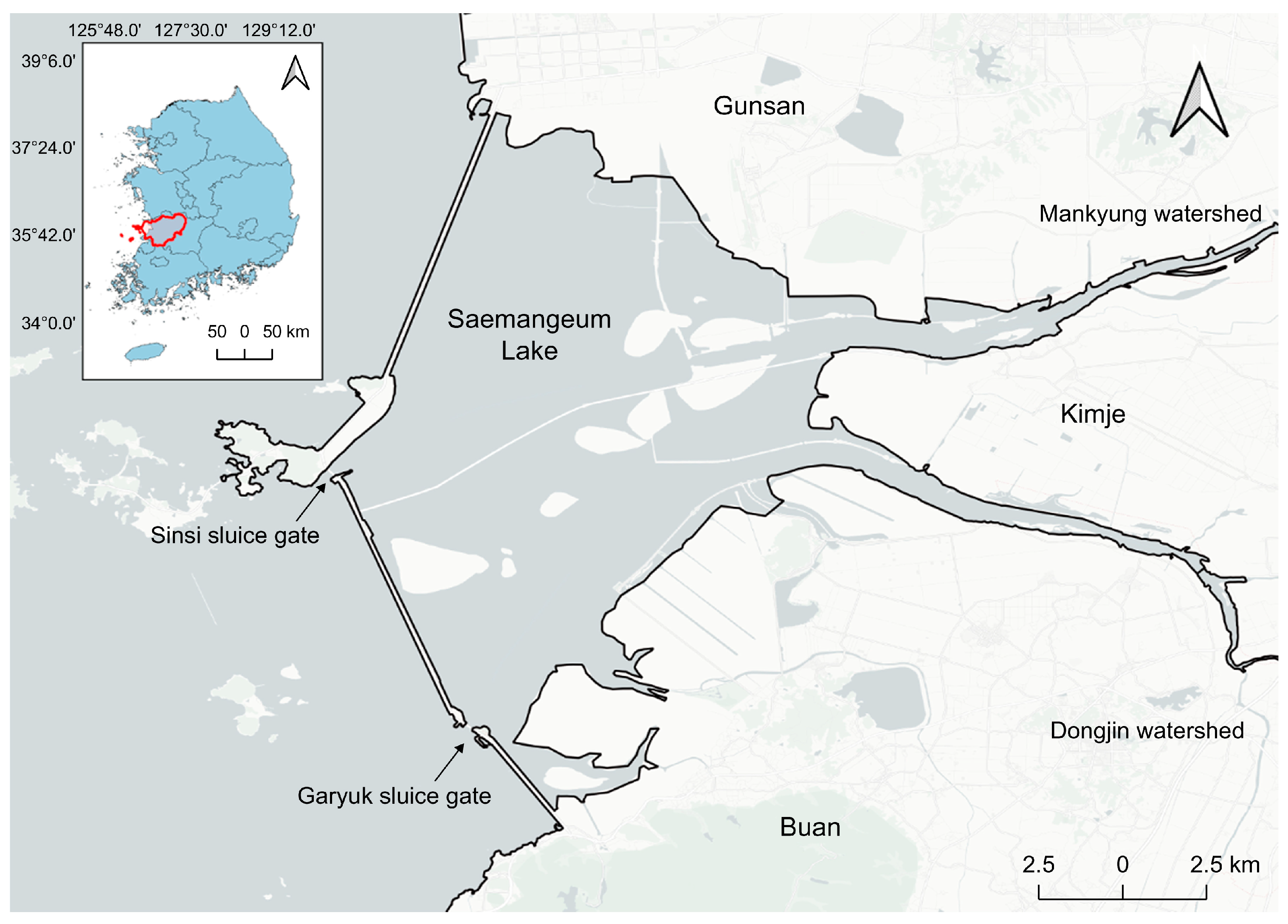
2.1. Study Area
2.2. Model Description
2.3. Model Construction
2.4. Water Body-Benthic Sediment Reaction Simulation Method
2.5. Model Assessment
2.6. Model Validation
2.7. Validation of Water Body-Benthic Sediment Reaction Simulation Method
3. Results and Discussion
Application of the Model
4. Conclusions
Author Contributions
Funding
Data Availability Statement
Conflicts of Interest
References
- Sahavacharin, A.; Sompongchaiyakul, P.; Thaitakoo, D.J.L. The Effects of Land-Based Change on Coastal Ecosystems. Landsc. Ecol. Eng. 2022, 18, 351–366. [Google Scholar] [CrossRef]
- Korea Environment Institute (KEI). A Study on the Development of Environmental Standards for Waterbed Sediments; Korea Environment Institute (KEI): Sejong, Republic of Korea, 2001. [Google Scholar]
- Lim, J.W.; Kwun, S.K. Development and Application of Multiple Box Water Quality Model for Estuary Reservoirs. J. Korean Soc. Agric. Eng. 1989, 31, 111–122. [Google Scholar]
- Portnoy, J.W. Summer Oxygen Depletion in a Diked New England Estuary. Estuaries 1991, 14, 122–129. [Google Scholar] [CrossRef]
- Lee, Y.S.; Lee, K.S. A Study on Release Characteristics of Sediment and Its Impacts on Water Quality in Daecheong Dam Reservoir. J. Environ. Impact Assess. 2000, 9, 99–107. [Google Scholar]
- Hsieh, C.D.; Yang, W.F. Optimal Nonpoint Source Pollution Control Strategies for a Reservoir Watershed in Taiwan. J. Environ. Manag. 2007, 85, 908–917. [Google Scholar] [CrossRef]
- Oh, K.; Chung, S.; Cho, Y. Analysis of Physicochemical Characteristics of Suspended Sediments Flowing into the Saemangeum Reservoir in the Summer. J. Korean Soc. Environ. Eng. 2015, 37, 99–106. [Google Scholar] [CrossRef]
- Yoo, S.C.; Suh, W.S.; Lee, H.Y. Impacts on Residence Time and Water Quality of the Saemangeum Reservoir Caused by Inner Development. J. Korean Soc. Mar. Environ. Energy 2012, 15, 186–197. [Google Scholar] [CrossRef]
- Korea Rural Community Corporation (KRC). Prediction Study on Water Quality Associated with the Changing of Saemangeum Project Condition; Korea Rural Community Corporation (KRC): Najusi, Republic of Korea, 2015. [Google Scholar]
- Wei, H.; Zhao, L.; Zhang, H.; Lu, Y.; Yang, W.; Song, G. Summer Hypoxia in Bohai Sea Caused by Changes in Phytoplankton Community. Anthr. Coasts 2021, 4, 77–86. [Google Scholar] [CrossRef]
- Hao, A.; Kobayashi, S.; Yan, N.; Xia, D.; Zhao, M.; Iseri, Y. Improvement of Water Quality Using a Circulation Device Equipped with Oxidation Carriers and Light Emitting Diodes in Eutrophic Pond Mesocosms. J. Environ. Chem. Eng. 2021, 9, 105075. [Google Scholar] [CrossRef]
- Malecki, L.M.; White, J.R.; Reddy, K.R. Nitrogen and Phosphorus Flux Rates from Sediment in the Lower St. Johns River Estuary. J. Environ. Qual. 2004, 33, 1545–1555. [Google Scholar] [CrossRef]
- Tufford, D.L.; McKellar, H.N. Spatial and Temporal Hydrodynamic and Water Quality Modeling Analysis of a Large Reservoir on the South Carolina (USA) Coastal Plain. Ecol. Modell. 1999, 114, 137–173. [Google Scholar] [CrossRef]
- Kung, H.T.; Ying, L.G. A Study of Lake Eutrophication in Shanghai, China. Geogr. J. 1991, 157, 45–50. [Google Scholar] [CrossRef]
- National Institute of Environmental Research (NIER). A Model Construction for Quantification on Water Quality Improvement Effect of Saeamangeum Area (II), Incheon, Korea. 2014; Environmental Digital Library (MOE). Available online: https://library.me.go.kr (accessed on 2 June 2023).
- Shin, S.; Her, Y.; Muñoz-Carpena, R.; Yu, X. Quantifying the Contribution of External Loadings and Internal Hydrodynamic Processes to the Water Quality of Lake Okeechobee. Sci. Total Environ. 2023, 883, 163713. [Google Scholar] [CrossRef] [PubMed]
- North Carolina Department of Environment and Natural Resources, Falls Lake Nutrient Response Model Final Report, North Carolina. 2009; North Carolina Environmental Quality. Available online: https://www.deq.nc.gov (accessed on 2 June 2023).
- Wang, Y.; Peng, Z.; Liu, G.; Zhang, H.; Zhou, X.; Hu, W. A Mathematical Model for Phosphorus Interactions and Transport at the Sediment-Water Interface in a Large Shallow Lake. Ecol. Model. 2023, 476, 110254. [Google Scholar] [CrossRef]
- Wang, Y.; Gao, X.; Sun, B.; Liu, Y. Developing a 3D Hydrodynamic and Water Quality Model for Floating Treatment Wetlands to Study the Flow Structure and Nutrient Removal Performance of Different Configurations. Sustainability 2022, 14, 7495. [Google Scholar] [CrossRef]
- Qin, Z.; He, Z.; Wu, G.; Tang, G.; Wang, Q. Developing Water-Quality Model for Jingpo Lake Based on EFDC. Water 2022, 14, 2596. [Google Scholar] [CrossRef]
- Rosario-Llantín, J.A.; Zarillo, G.A. Flushing Rates and Hydrodynamical Characteristics of Mosquito Lagoon (Florida, USA). Environ. Sci. Pollut. Res. Int. 2021, 28, 30019–30034. [Google Scholar] [CrossRef]
- Yildiz, K.; Karakaya, N.; Kilic, S.; Evrendilek, F. Interaction Effects of the Main Drivers of Global Climate Change on Spatiotemporal Dynamics of High Altitude Ecosystem Behaviors: Process-Based Modeling. Environ. Monit. Assess. 2020, 192, 457. [Google Scholar] [CrossRef]
- Khadka, P.; Sharma, S.; Mathis, T. Monitoring an Ungagged Coastal Marsh to Analyze the Salinity Interaction of the Marsh with Lake Erie. Environ. Monit. Assess. 2021, 193, 645. [Google Scholar] [CrossRef]
- Luo, X.; Li, X. Using the EFDC Model to Evaluate the Risks of Eutrophication in an Urban Constructed Pond from Different Water Supply Strategies. Ecol. Modell. 2018, 372, 1–11. [Google Scholar] [CrossRef]
- Choi, J.; Oh, C.; Kweon, Y.; Ahn, C. Consideration on the Operation of water level management and Environmental Change Associated with Inner Dike Constructions in Saemangeum Reservoir. J. Korean Soc. Mar. Environ. Energy 2013, 16, 290–298. [Google Scholar] [CrossRef] [Green Version]
- Korea Rural Community Corporation (KRC). Ecological Changes in the Saemangeum Water and Reclaimed Land Areas (IV); Korea Rural Community Corporation (KRC): Najusi, Republic of Korea, 2009. [Google Scholar]
- Hamrick, J.M. A Three-Dimensional Environmental Fluid Dynamics Computer Code: Theoretical and Computational Aspects. 63 Williamsburg; Special Report 317; College of William and Mary, Virginia Institute of Marine Science: Williamsburg, VA, USA, 1992. [Google Scholar]
- Tetra Tech, Inc. The Environmental Fluid Dynamics Code Theory and Computation Volume 1: Hydrodynamics and Mass Transport; Tetra Tech Inc.: Fairfax, VA, USA, 2007. [Google Scholar]
- Tetra Tech, Inc. The Environmental Fluid Dynamics Code Theory and Computation Volume 3: Water Quality Module; Tetra Tech Inc.: Fairfax, VA, USA, 2007. [Google Scholar]
- Ministry of Land, Infrastructure and Transport (MLIT). Preliminary Investigation on Securing and Procurement of Saemangeum Landfill; Ministry of Land, Infrastructure and Transport (MLIT): Sejong, Republic of Korea, 2011.
- Matsumoto, K.; Takanezawa, T.; Ooe, M. Ocean Tide Models Developed by Assimilating TOPEX/POSEIDON Altimeter Data into Hydrodynamical Model: A Global Model and a Regional Model Around Japan. J. Oceanogr. 2000, 56, 567–581. [Google Scholar] [CrossRef]
- Makinde, O.O.; Edun, O.M.; Akinrotimi, O.A. Comparative Assessment of Physical and Chemical Characteristics of Water in Ekerekana and Buguma Creeks, Niger Delta, Nigeria. J. Environ. Prot. Sustain. Dev. 2015, 1, 126–133. [Google Scholar]
- Ejigu, M.T. Overview of Water Quality Modeling. Cogent Eng. 2021, 8, 1891711. [Google Scholar] [CrossRef]
- Chapra, S.C. Surface Water Quality Modeling; Tufts University: Medford, MA, USA, 1996. [Google Scholar]
- Wang, C.; Liu, S.; Shi, X.; Cui, G.; Wang, H.; Jin, X.; Fan, K.; Hu, S. Numerical Modeling of Contaminant Advection Impact on Hydrodynamic Diffusion in a Deformable Medium. J. Rock Mech. Geotech. Eng. 2022, 14, 994–1004. [Google Scholar] [CrossRef]
- Ministry of the Environment (MOE). Study on Master Plan for Water Quality Improvement in Saemangeum Basin; Ministry of the Environment (MOE): Sejong, Republic of Korea, 2011.
- Haas, A.F.; Smith, J.E.; Thompson, M.; Deheyn, D.D. Effects of Reduced Dissolved Oxygen Concentrations on Physiology and Fluorescence of Hermatypic Corals and Benthic Algae. PeerJ 2014, 2, e235. [Google Scholar] [CrossRef]
- Jiang, X.; Jin, X.; Yao, Y.; Li, L.; Wu, F. Effects of Biological Activity, Light, Temperature and Oxygen on Phosphorus Release Processes at the Sediment and Water Interface of Taihu Lake, China. Water Res. 2008, 42, 2251–2259. [Google Scholar] [CrossRef] [PubMed]
- Zhang, M.; Li, Y.; Wang, H.; Yu, Y.; Liu, J.; Qiao, R.; Liu, M.; Ma, S.; Wang, H. Decreased Internal Phosphorus Loading from Eutrophic Sediment After Artificial Light Supplement: Preliminary Evidence from a Microcosm Experiment. Front. Environ. Sci. 2022, 10, 148. [Google Scholar] [CrossRef]
- Jiang, H.Z.; Shen, Y.M.; Wang, S.D. Numerical Study on Salinity Stratification in the Oujiang River Estuary. J. Hydrodyn. 2009, 21, 835–842. [Google Scholar] [CrossRef]
- Huang, F.; Lin, X.; Yin, K.J.E.I. Effects of Algal-Derived Organic Matter on Sediment Nitrogen Mineralization and Immobilization in a Eutrophic Estuary. Ecol. Indic. 2022, 138, 108813. [Google Scholar] [CrossRef]
- Sun, Q.; Wang, S.; Zhou, J.; Chen, Z.; Shen, J.; Xie, X.; Wu, F.; Chen, P. Sediment Geochemistry of Lake Daihai, North-Central China: Implications for Catchment Weathering and Climate Change During the Holocene. J. Paleolimnol. 2010, 43, 75–87. [Google Scholar] [CrossRef]
- Miranda, L.S.; Ayoko, G.A.; Egodawatta, P.; Goonetilleke, A. Adsorption-Desorption Behavior of Heavy Metals in Aquatic Environments: Influence of Sediment, Water and Metal Ionic Properties. J. Hazard. Mater. 2022, 421, 126743. [Google Scholar] [CrossRef]
- Bai, J.; Ye, X.; Jia, J.; Zhang, G.; Zhao, Q.; Cui, B.; Liu, X. Phosphorus Sorption-Desorption and Effects of Temperature, pH and Salinity on Phosphorus Sorption in Marsh Soils from Coastal Wetlands with Different Flooding Conditions. Chemosphere 2017, 188, 677–688. [Google Scholar] [CrossRef]
- Zhang, H.; Elskens, M.; Chen, G.; Chou, L. Phosphate Adsorption on Hydrous Ferric Oxide (HFO) at Different Salinities and pHs. Chemosphere 2019, 225, 352–359. [Google Scholar] [CrossRef] [PubMed]
- Lehtoranta, J.; Ekholm, P.; Pitkänen, H. Coastal eutrophication thresholds: A matter of sediment microbial processes. AMBIO A J. Hum. Environ. 2009, 38, 303–308. [Google Scholar] [CrossRef] [PubMed]
- Hansel, C.M.; Lentini, C.J.; Tang, Y.; Johnston, D.T.; Wankel, S.D.; Jardine, P.M. Dominance of Sulfur-Fueled Iron Oxide Reduction in Low-Sulfate Freshwater Sediments. ISME J. 2015, 9, 2400–2412. [Google Scholar] [CrossRef]
- Reed, D.C.; Slomp, C.P.; Gustafsson, B.G.J.L. Sedimentary Phosphorus Dynamics and the Evolution of Bottom--Water Hypoxia: A Coupled Benthic–Pelagic Model of a Coastal System. Limnol. Oceanogr. 2011, 56, 1075–1092. [Google Scholar] [CrossRef]
- Boström, B.; Andersen, J.M.; Fleischer, S.; Jansson, M. Exchange of Phosphorus across the Sediment-Water Interface. Hydrobiologia 1988, 170, 229–244. [Google Scholar] [CrossRef]
- Coelho, J.P.; Flindt, M.R.; Jensen, H.S.; Lillebø, A.I.; Pardal, M.A. Phosphorus Speciation and Availability in Intertidal Sediments of a Temperate Estuary: Relation to Eutrophication and Annual P-Fluxes. Estuar. Coast. Shelf Sci. 2004, 61, 583–590. [Google Scholar] [CrossRef] [Green Version]
- Ministry of the Environment (MOE). Sediment Monitoring of the Saemangeum Lake; Ministry of the Environment (MOE): Sejong, Republic of Korea, 2018.
- Moriasi, D.N.; Arnold, J.G.; Van Liew, M.W.; Bingner, R.L.; Harmel, R.D.; Veith, T.L. Model Evaluation Guidelines for Systematic Quantification of Accuracy in Watershed Simulations. Trans. ASABE 2007, 50, 885–900. [Google Scholar] [CrossRef]
- Tasnim, B.; Fang, X.; Hayworth, J.S.; Tian, D. Simulating Nutrients and Phytoplankton Dynamics in Lakes: Model Development and Applications. Water 2021, 13, 2088. [Google Scholar] [CrossRef]
- Chapra, S.C.; Dobson, H.F.H. Quantification of the Lake Trophic Typologies of Naumann (Surface Quality) and Thienemann (Oxygen) with Special Reference to the Great Lakes. J. Gr. Lakes Res. 1981, 7, 182–193. [Google Scholar] [CrossRef]
- Masson-Delmotte, V.; Zhai, P.; Pirani, A.; Connors, S.L.; Péan, C.; Berger, S.; Caud, N.; Chen, Y.; Goldfarb, L.; Gomis, M.I.; et al. IPCC, 2021: Climate Change 2021: The Physical Science Basis. Contribution of Working Group I to the Sixth Assessment Report of the Intergovernmental Panel on Climate Change; Cambridge University Press: Cambridge, UK; New York, NY, USA, 2021; in press. [Google Scholar]
- Lee, H.; Romero, J. IPCC, 2023: Climate Change 2023: Synthesis Report. A Report of the Intergovernmental Panel on Climate Change. Contribution of Working Groups I, II and III to the Sixth Assessment Report of the Intergovernmental Panel on Climate Change; Core Writing Team, Ed.; IPCC: Geneva, Switzerland, 2023; in press. [Google Scholar]


| Parameters | Unit | Definition | Calibration |
|---|---|---|---|
| PMc, PMd, PMs | /day | maximum growth rate under optimal conditions for algal group x | 2.8 |
| KHNx | /gNm3 | half-saturation constant for nitrogen uptake for algal group x | 0.01 |
| KHPx | /gPm3 | half-saturation constant for phosphorus uptake for algal group x | 0.001 |
| KHS | /gSim3 | half-saturation constant for silica uptake for diatoms | 0.05 |
| CCHlx | gC/mgChl | carbon-to-chlorophyll ratio in algal group x | 0.03 |
| TMc1, TMd1, TMg1 | °C | optimal temperature for algal growth for algal group x | 20.0 |
| TMc2 | °C | optimal temperature for algal growth for algal group x | 27.5 |
| TMd2, TMg2 | 25.0 | ||
| BFPO4d | - | sediment-water exchange flux of phosphate (g P/m2/day) | 0.009 |
| WSS | m/day | settling velocity of particulate metal | 1.0 |
| KRP | /day | minimum hydrolysis rate of refractory particulate organic phosphorus | 0.15 |
| KLP | /day | minimum hydrolysis rate of labile particulate organic phosphorus | 0.0175 |
| KDP | /day | minimum mineralization rate of dissolved organic phosphorus | 0.001 |
| Kcd | /day | oxidation rate of chemical oxygen demand at TRCOD | 20 |
| BFCOD | - | benthic flux rate of chemical oxygen demand | 0.12 |
| KRN | /day | minimum hydrolysis rate of refractory particulate organic nitrogen | 0.075 |
| KLN | /day | minimum hydrolysis rate of labile particulate organic nitrogen | 0.175 |
| KDN | /day | minimum mineralization rate of dissolved organic nitrogen | 0.001 |
| BFNH4 | - | benthic flux rate of ammonia nitrogen | 0.009 |
| WSRP | m/day | settling velocity of refractory particulate organic matter | 0.55 |
| WSLP | m/day | settling velocity of labile particulate organic matter | 0.55 |
| KRC | /day | minimum dissolution rate of refractory particulate organic carbon | 0.075 |
| KLC | /day | minimum dissolution rate of labile particulate organic carbon | 0.175 |
| KDC | /day | minimum respiration rate of dissolved organic carbon | 0.01 |
| ASCd | gSi/gC | silica-to-carbon ratio of diatoms | 0.05 |
| KSU | /day | dissolution rate of particulate biogenic silica | 0.05 |
| Classification | Station | Water Temperature (°C) | Salinity (psu) | ||
|---|---|---|---|---|---|
| Aerobic | Anaerobic | ||||
| 1st | ME2 | 0.1317 | 0.1528 | 26.5 | 2.80 |
| ML3 | 0.0191 | 0.0216 | 23.8 | 23.8 | |
| MK7 | 0.1311 | 0.1884 | 21.2 | 21.2 | |
| DE2 | 0.0561 | 0.0504 | 26.9 | 1.20 | |
| DL2 | 0.0178 | 0.0302 | 19.5 | 19.5 | |
| 2nd | ME2 | 0.0280 | 0.0382 | 15.3 | 9.40 |
| ML3 | 0.0176 | 0.0270 | 15.2 | 25.5 | |
| MK7 | 0.0048 | 0.0230 | 14.0 | 24.0 | |
| DE2 | 0.0115 | 0.0053 | 16.7 | 6.6 | |
| DL2 | 0.0433 | 0.0744 | 14.7 | 22.8 | |
| 3rd | ME2 | 0.047 | 0.0332 | 15.5 | 12.1 |
| ML3 | 0.1273 | 0.0248 | 12.6 | 30.5 | |
| MK7 | 0.0069 | 0.0346 | 12.1 | 30.7 | |
| DE2 | 0.0145 | 0.0247 | 15.6 | 17.0 | |
| DL2 | 0.0112 | 0.0491 | 12.9 | 22.6 | |
| 4th | ME2 | 0.0458 | 0.0710 | 28.1 | 3.4 |
| ML3 | 0.0223 | 0.0223 | 28.1 | 17.3 | |
| MK7 | 0.0119 | 0.0159 | 29.6 | 12.1 | |
| DE2 | 0.0178 | 0.0601 | 27.7 | 0.8 | |
| DL2 | 0.0046 | 0.0178 | 28.0 | 19.4 | |
| 5th | ME2 | 0.1589 | 0.330 | 9.6 | 7.4 |
| ML3 | 0.0244 | 0.06898 | 4.8 | 30.7 | |
| MK7 | 0.0344 | 0.0447 | 4.8 | 30.7 | |
| DE2 | 0.0009 | 0.0285 | 5.8 | 18.3 | |
| DL2 | 0.1635 | 0.1184 | 4.8 | 29.2 | |
| Criteria | Equation | Optimal Value |
|---|---|---|
| RSR | 0 | |
| % Difference | 0 | |
| AME | 0 |
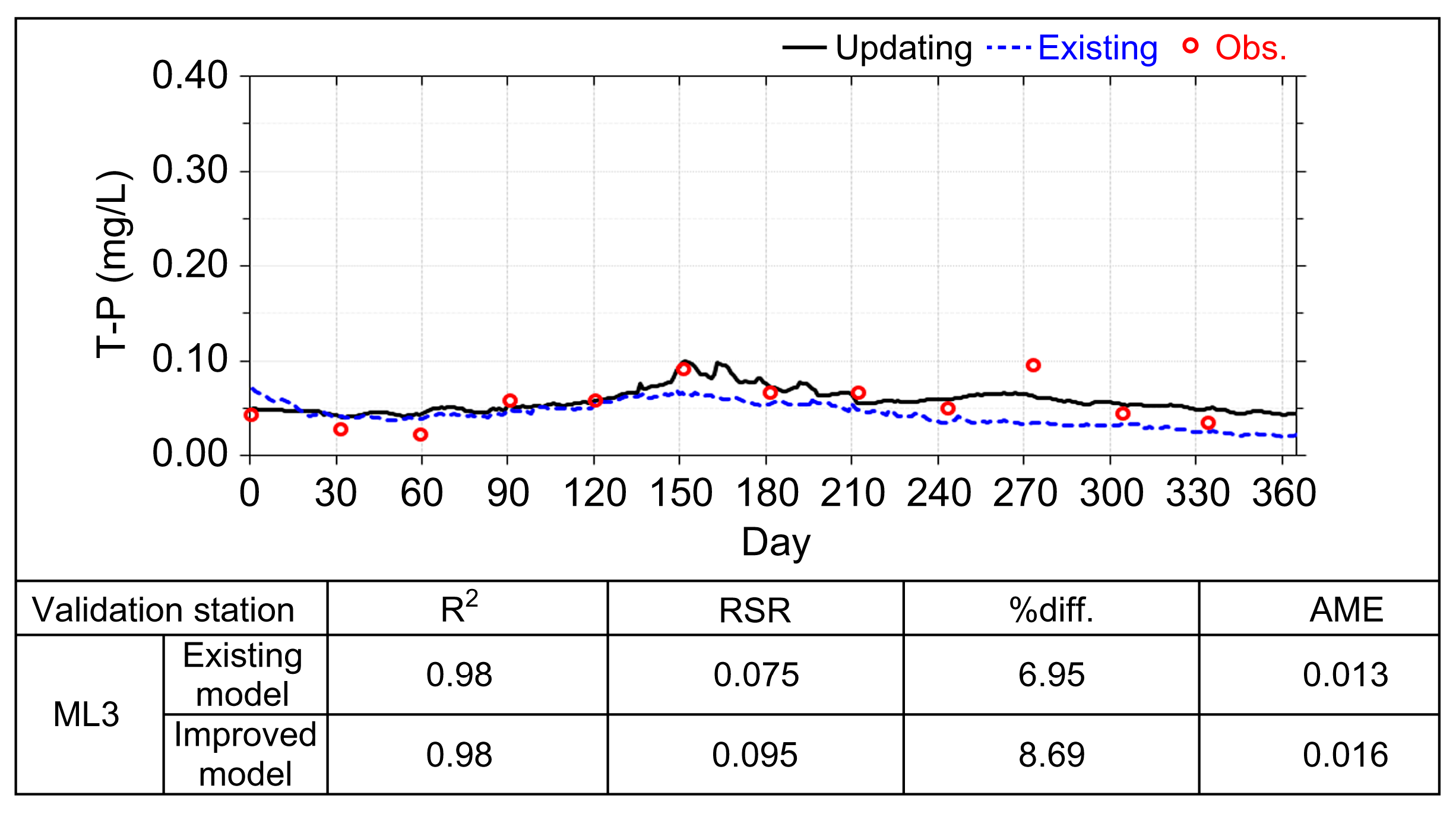
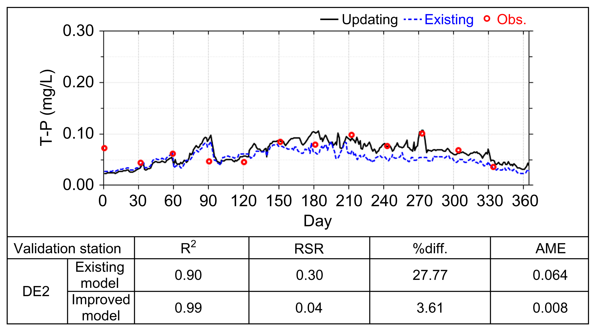
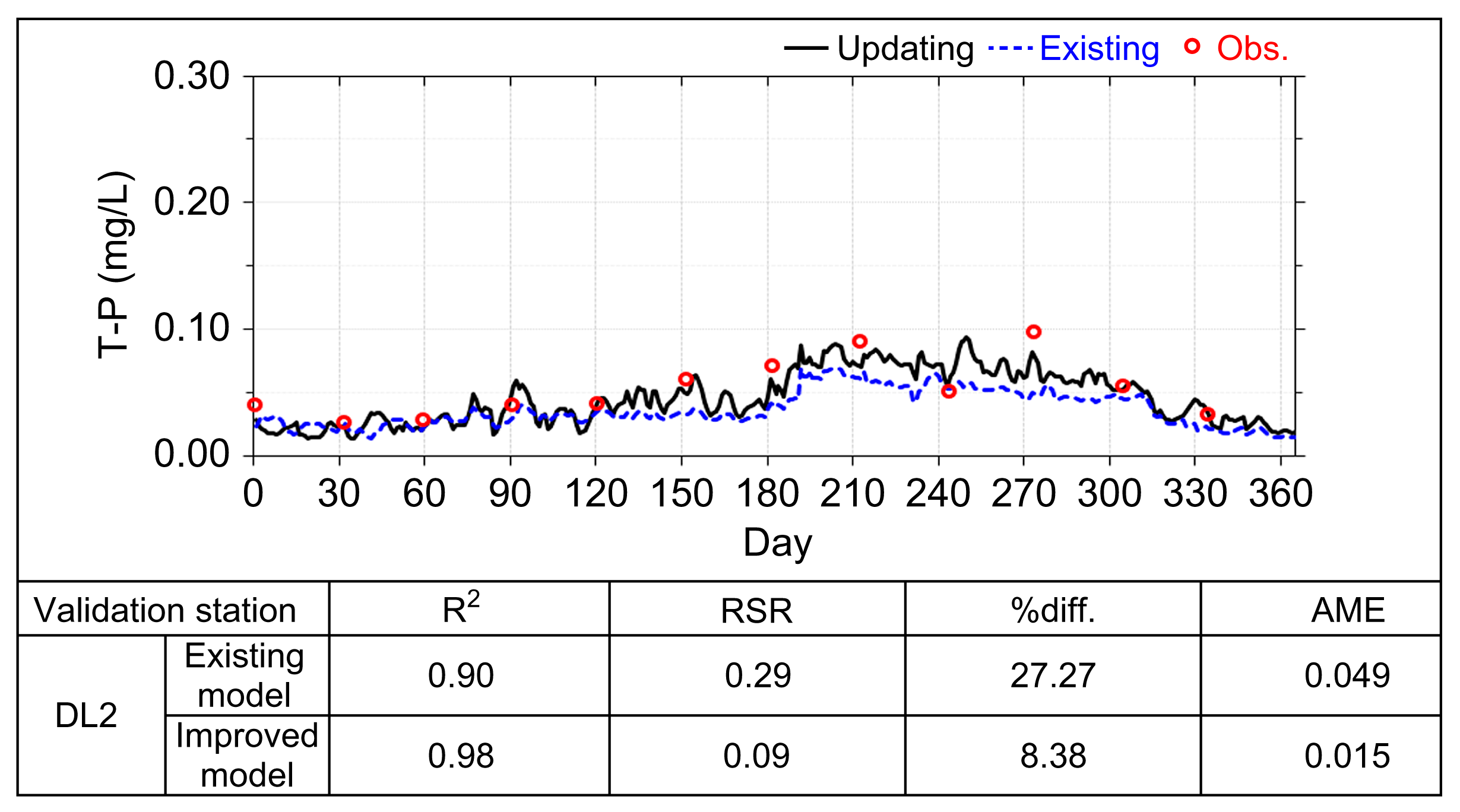
| Validation Stations | RSR | %diff. | AME | |
|---|---|---|---|---|
| DO | ME2 | 0.029 | 2.7 | 0.241 |
| ML3 | 0.066 | 6.0 | 0.501 | |
| DE2 | 0.204 | 18.7 | 1.491 | |
| DL2 | 0.003 | 0.3 | 0.022 | |
| Chl-a | ME2 | 0.123 | 11.2 | 3.955 |
| ML3 | 0.480 | 44.0 | 5.909 | |
| DE2 | 0.361 | 33.1 | 9.697 | |
| DL2 | 1.596 | 146.3 | 22.549 | |
| T-N | ME2 | 0.134 | 12.3 | 0.353 |
| ML3 | 0.295 | 27.0 | 0.214 | |
| DE2 | 0.139 | 12.7 | 0.209 | |
| DL2 | 0.115 | 10.6 | 0.101 | |
| T-P | ME2 | 0.027 | 2.5 | 0.003 |
| ML3 | 0.471 | 43.2 | 0.020 | |
| DE2 | 0.157 | 14.4 | 0.013 | |
| DL2 | 0.083 | 7.6 | 0.004 | |
| COD | ME2 | 0.118 | 10.9 | 0.773 |
| ML3 | 0.110 | 10.1 | 0.394 | |
| DE2 | 0.146 | 13.4 | 0.833 | |
| DL2 | 0.009 | 0.8 | 0.035 | |
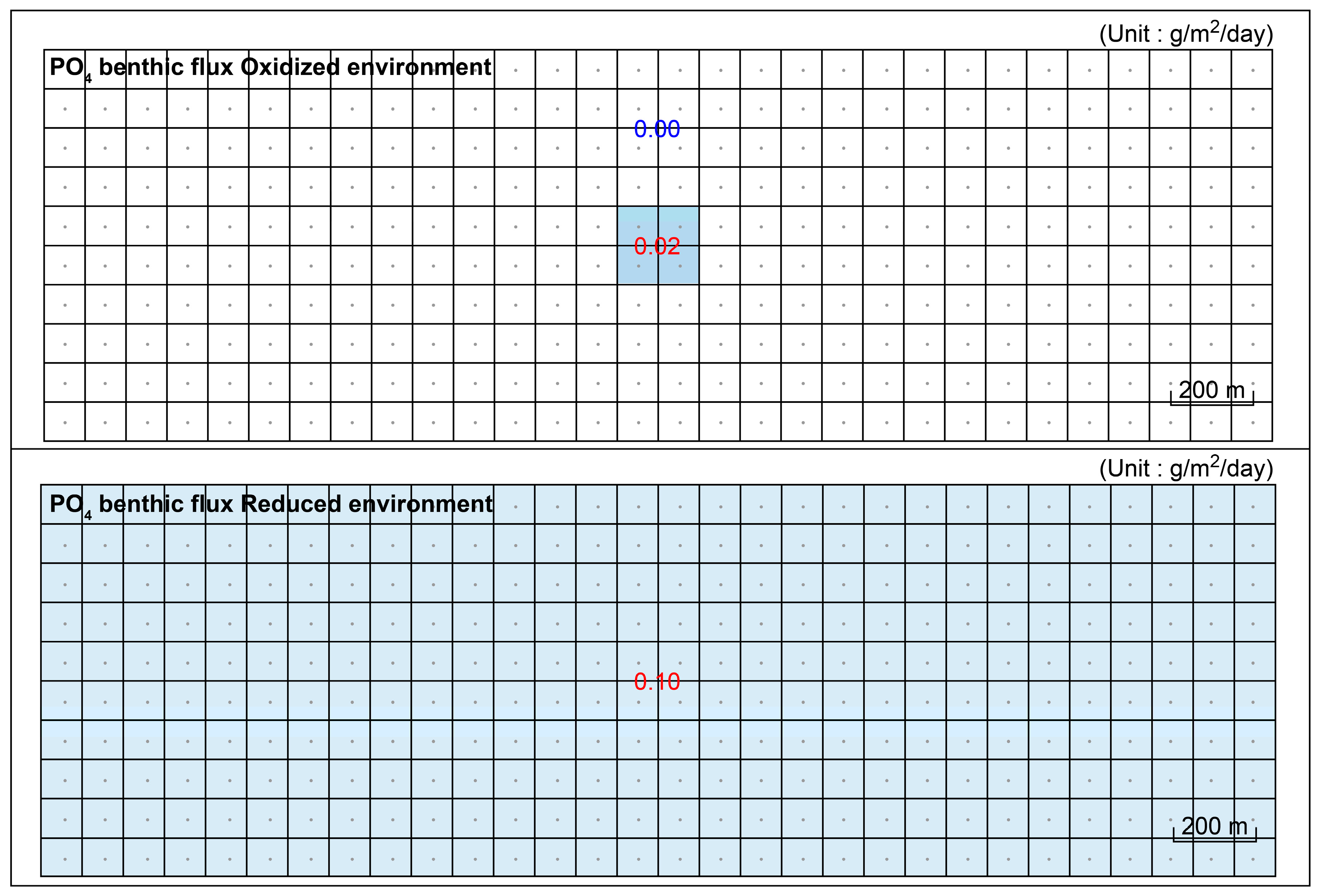
| Experiment Cases | Applied Model | Vertical Mixing | Release Zone | Flux Rate (g/m2/day) | ||
|---|---|---|---|---|---|---|
| SOD | PO4 | |||||
| Aerobic (Oxidized) | Anaerobic (Reduced) | |||||
| Case 1 | Existing | × | × | −2.0 | 0.02 | |
| Case 2 | Improved | × | × | −2.0 | 0.02 | 0.10 |
| Case 3 | Improved | ○ | × | −2.0 | 0.02 | 0.10 |
| Case 4-1 Case 4-2 | Improved | ○ | ○ | −2.0 | (Zone 1) 0.02 (Zone 2) 0.00 | (Zone 1) 0.10 (Zone 2) 0.10 |
| Item | Description | |
|---|---|---|
| Purpose of experiment | Simulation of total phosphorus changes according to improved method of applying the flux rate | |
| Scope of the model | 64 km in the east-west direction, and 54 km in the south-north direction | |
| Model configuration | Grid configuration | Orthogonal Curvilinear Coordinate |
| Number of grids | 5897 | |
| Experimental conditions | Open boundary | Composite tides of the four main sub-tidal currents (M2, S2, K1, O1) |
| Calculation interval | △t = 6 s | |
| Experiment period | 1 January 2016–31 December 2016 | |
| Experimental condition | (Existing model) flux rate: 0.003 g/m2/day(Improved model) flux rate: spatiotemporal flux rate according to water temperature-salinity changes | |
Disclaimer/Publisher’s Note: The statements, opinions and data contained in all publications are solely those of the individual author(s) and contributor(s) and not of MDPI and/or the editor(s). MDPI and/or the editor(s) disclaim responsibility for any injury to people or property resulting from any ideas, methods, instructions or products referred to in the content. |
© 2023 by the authors. Licensee MDPI, Basel, Switzerland. This article is an open access article distributed under the terms and conditions of the Creative Commons Attribution (CC BY) license (https://creativecommons.org/licenses/by/4.0/).
Share and Cite
Kim, S.; Park, Y. An Improved Model for Water Quality Management Accounting for the Spatiotemporal Benthic Flux Rate. Water 2023, 15, 2219. https://doi.org/10.3390/w15122219
Kim S, Park Y. An Improved Model for Water Quality Management Accounting for the Spatiotemporal Benthic Flux Rate. Water. 2023; 15(12):2219. https://doi.org/10.3390/w15122219
Chicago/Turabian StyleKim, Semin, and Youngki Park. 2023. "An Improved Model for Water Quality Management Accounting for the Spatiotemporal Benthic Flux Rate" Water 15, no. 12: 2219. https://doi.org/10.3390/w15122219