A Random Forest Machine Learning Approach for the Identification and Quantification of Erosive Events

Abstract

Predicting the occurrence of erosive rain events and quantifying the corresponding soil loss is extremely useful in all applications where assessing phenomenon impacts is required. These problems, addressed in the literature at different spatial and temporal scales and according to the most diverse approaches, are here addressed by implementing random forest (RF) machine learning models. For this purpose, we used the datasets built through many years of soil loss observations at the plot-scale experimental site SERLAB (central Italy). Based on 32 features describing rainfall characteristics, the RF classifier has achieved a global accuracy of 84.8% in recognizing erosive and non-erosive events, thus demonstrating slightly higher performances than previously used (non-machine learning) methodologies. A critical performance is the percentage of erosive events correctly recognized to the observed total (72.3%). However, since the most relevant erosive events are correctly identified, we found only a slight underestimation of the total rainfall erosivity (91%). The RF regression model for estimating the event soil loss, based on three event features (runoff coefficient, erosivity, and period of occurrence), demonstrates better performances (RMSE = 2.30 Mg ha⁻¹) than traditional regression models (RMSE = 3.34 Mg ha⁻¹).

1. Introduction

In its accelerated forms, soil water erosion leads to several adverse on-site (loss of nutrients and organic matter, permeability) and off-site (pollution of water bodies, destruction of habitats, siltation of water bodies and flood risk increase) effects [1,2]. The effectiveness of environmental programs and policies or specific soil erosion control strategies strictly depends on the knowledge of the complex mechanism and factors conditioning the occurrence and the extent of erosive processes. This knowledge necessarily derives from the availability of adequate datasets (with the fundamental contribution of experimental and monitoring activities) and appropriate modelling approaches. Among the numerous model types (empirical, conceptual, physically based, or process-oriented) proposed in the literature to estimate soil loss at different spatial and temporal scales, empirical models are still the most used due to their capacity to combine simplicity and reliability [3,4]. In particular, the Universal Soil Loss Equation (USLE, [5]) or its revised version (Revised USLE, RUSLE, [6]) are the most widely applied models to predict long-term average soil loss values. They are also considered the standard applications of soil conservation workers [7,8]. However, since a large proportion of soil loss is due to a few particularly erosive events [9,10,11], mitigation and management strategies should rely on models capable of predicting event-scale erosion rather than the long-term average. Various studies have moved in this direction [12,13,14,15], proposing changes to the USLE approach (or subsequent revisions) to make it reliable on the single-event scale. These changes usually consist of the use of an erosivity index given by the combination of the event runoff coefficient, Q_R (dimensionless), and the single-storm erosion index, E·I30 = R (MJ mm ha⁻¹ h⁻¹) by Wischmeier and Smith [5]. For example, the studies conducted to date at various Italian plot scale experimental sites [4,10,16] have proposed and tested a model (named USLE-MM) of the following type:

$$A_e={\left(Q_R·R\right)}^{b1}{K}_{UMM}LS{C}_{UMM}{P}_{UMM}$$

(1)

where A_e (Mg ha⁻¹) is the event soil loss per unit area, L and S (dimensionless) are, respectively, the USLE slope length and steepness factors, K_UMM (Mg ha h ha⁻¹ MJ⁻¹ mm⁻¹) is the soil erodibility factor, C_UMM (dimensionless) is the cover and management factor, P_UMM (dimensionless) is the support practice factor, and b1 is an exponent to be parametrized based on collected data. Although the model of Equation (1) demonstrates decidedly superior performance at the event scale to the original USLE (which suffers from a systematic bias, [12]), there is still a large portion of unexplained variance, which stimulates both the continuation of the monitoring activities and the search for new modelling approaches.

In addition to modelling soil loss, the literature has long investigated the possibility of identifying erosive events based only on rainfall characteristics. This information may be helpful in various research and practical applications. For example, it allows us to determine the triggering of erosion processes of different entities and consequently to understand their dynamics better; reduces the work necessary to manage and process erosive events; allows us to study the spatio-temporal frequency of erosive events [17]. The first reference in this context is that in [5], which indicated as erosive the rainfalls capable of exceeding the depth thresholds of 12.7 mm or 6.35 mm in 15 min. More recent studies [17,18,19] have searched for such a type of thresholds in large datasets of variables characterizing, not only considering the overall characteristics of rainfall (e.g., depth, duration), but also their internal structure (e.g., presence and duration of high-intensity showers). For example, Todisco et al. [17], based on the data observed at the Masse (central Italy) and Sparacia (south Italy) experimental sites, demonstrated that some of these variables could effectively classify non-erosive and erosive events and even separate erosive events that produce sheet or rill erosion.

Both the classification and the quantification of erosion processes, which are physically very complex and depend on many concomitant and interacting factors, can certainly be tackled with good prospects using artificial intelligence and machine learning technologies. These approaches have been increasingly applied in all scientific areas [20] as a result of their ability to process large amounts of data in a relatively simple way and identify complex patterns and relationships from the data itself to make reliable predictions on data not seen before. This strength is, at the same time, also a weakness, as without large enough datasets to train on, such models provide inaccurate estimates. Applications in the field of soil erosion processes mainly refer to the use of artificial neural network (ANN) models, usually applied to predict runoff and soil loss [21,22,23,24,25] or other erosion-related factors [26]. Among the various machine learning techniques, the random forest (RF) is increasingly applied as a result of its several advantageous characteristics, such as the relative ease of managing large datasets, the possibility of using nominal and numerical data, the high accuracy of the predictions, and the possibility of being used for both classification and regression problems [27]. Overfitting, which happens when a model is too focused on the training data and fails to generalize well to new data, is less likely to occur in RF than in ANN [28]. This is due to the bootstrap and randomized feature sampling used in RF algorithm. Moreover, although both RF and ANN appear as “black boxes”, RF allows a more straightforward interpretation of the factors affecting the prediction. RF algorithms have been used with promising results in several research fields related to hydraulics and hydrology [29], such as pipe breaks in water supply networks [30], water flow in porous media [31], flooding [32] and drought [33] events. RF applications in soil water erosion studies are limited in the literature and, therefore, can be considered quite innovative. One of the few examples is the recent work by Tarek et al. [34], demonstrating the higher accuracy of the RF approach compared to other machine learning methods in the classification of erosive events.

This work aims to develop and evaluate RF algorithms for classifying erosive and non-erosive rain events and quantifying the soil loss at the single event time scale and plot spatial scale. The study is based on the large datasets obtained over many years of soil erosion monitoring at the Soil Erosion LABoratory (SERLAB) experimental site. By comparison with the results obtained from more traditional empirical methods, the good potential of RF algorithms in this type of application is demonstrated.

2. Materials and Methods

2.1. Experimental Site

In the study, we used the data collected at the Masse experimental site (42°59′34″ N 12°17′27″ E) of the Department of Agricultural, Food and Environmental Sciences of the University of Perugia. This site (Figure 1), also known as Soil Erosion LABoratory (SERLAB), was established in 2007 to monitor and characterize erosive processes at plot scale in central Italy’s typical agricultural context dominated by hills. The average annual rainfall is about 900 mm, and the soil is silt–clay–loam (clay = 34%, silt = 59%, and sand = 7%). Organic matter content is about 1%, and the gravel content is negligible. There are currently 10 Wischmeier-type plots of various sizes (four plots 22 × 8 m², two plots 22 × 4 m², two plots 11 × 4 m² and two plots 11 × 2 m²) with a 16% slope. The plots are kept in cultivated fallow through frequent tillage operations to remove vegetation and restore soil surface structure after erosive events. Each plot is equipped in its terminal part with a channel conveying solid and liquid runoff into 1-m³ storage tanks, the number of which varies with the plot size. After each erosive event (or occasionally, after a series of events if they are close to one another), the runoff and soil loss are measured with a specially calibrated sampling technique [35], and the tanks are emptied and cleaned to be ready to receive the runoff of a new event. The SERLAB meteorological station has several weather instrumentations, including a tipping bucket rain gauge set to record rainfall depths with a 5 min time step.

2.2. Datasets

The study relies on two datasets (DB1 and DB2), built with rainfall and soil loss data collected over several years of monitoring at the SERLAB site. The characteristics of the two datasets are detailed in the following sections.

2.2.1. Dataset (DB1) Used for the RF Classifier

For the development of an RF algorithm capable of classifying erosive and non-erosive events, we used the same dataset (DB1) considered in previous studies aimed at identifying the best rainfall variables (and the corresponding thresholds), able to separate erosive and non-erosive events [17,19,36]. The DB1 dataset includes 528 events (158 erosive and 370 non-erosive). The decision to consider the same dataset allows for a more straightforward comparison of the RF algorithm with other classification techniques applied recently. The dataset DB1 was built according to the steps detailed below.

The 5 min rainfall records from 1 January 2008 to 31 December 2017 were analysed to identify the individual storms, i.e., the rain events preceded and followed by 6 h or more of no rain (according to Wischmeier and Smith [5]).

Each individual storm was therefore categorized as erosive (E) if a measurable soil loss was found in the storage tanks, while it was considered non-erosive (NE) if it did not produce runoff or if the soil loss was so irrelevant that it could not be measured. Sometimes, when individual events are very close, soil loss refers to a sequence of individual storms. In this case, the individual storms included in the sequence were classified as non-erosive (erosive) if their rainfall depth was lower (higher) than the minimum depth observed for the individual erosive rainfalls [17].

For each individual storm, 31 variables (

Table A1. List of the features used in the training of the random forest classifier for the separation of erosive and non-erosive storms.

Variable	Symbol	Unit
Total rainfall	P	mm
Total duration	D	h
Wet duration	D_wet	h
Dry duration	D_dry	h
Mean intensity	I	mm h−1
Mean wet intensity	I_wet	mm h−1
Rainfall erosivity	R	MJ mm ha−1 h−1
Rainfall kinetic energy	E	MJ ha−1
Maximum intensity over 30 min	I30	mm h−1
Maximum intensity over 5 min	I5	mm h−1
Maximum intensity over 10 min	I10	mm h−1
Maximum intensity over 15 min	I15	mm h−1
Maximum intensity over 20 min	I20	mm h−1
Maximum intensity over 25 min	I25	mm h−1
Maximum intensity over 40 min	I40	mm h−1
Maximum intensity over 50 min	I50	mm h−1
Maximum intensity over 60 min	I60	mm h−1
Rainfall amount above truncation level p0	P_run	mm
Rainfall duration above truncation level p0	D_run	h
Number of runs	N_run	-
Maximum duration of an individual run	Max_D_run	h
Maximum rainfall amount of an individual run	Max_P_run	mm
Maximum peak of the run (p-p0)	Max_peak_run	mm
Maximum rainfall depth from the start of the storm to a run	Max_P_pre_run	mm
Maximum slope of the rising limb of a burst	Max_slope_burst	%
Maximum mean run intensity	Max_I_run	mm h−1
Number of bursts in a storm	N_burst	-
Maximum rainfall amount in a burst	Max_P_burst	mm
Maximum burst duration	Max_D_burst	h
Maximum rainfall depth from the start of the event to a burst	Max_P_pre_burst	mm
Maximum mean burst intensity	Max_I_burst	mm h−1
Period of occurrence	Period	-

) describing the hyetograph’s overall and pattern characteristics were quantified. In particular, the internal storm structure is represented by the characteristics (number, duration, severity, etc.) of bursts (i.e., intervals of continuous rain) and runs (i.e., intervals of continuous rain exceeding a predetermined truncation value p0). The identification of the truncation level, p0, was based on the frequency analysis of rainfall records by excluding zero values. The selected p0 value corresponds to a cumulative frequency of 95% [17], giving p0 = 0.8 mm in 5 min (9.6 mm/h). More calculation details about the rainfall variables can be found in Todisco et al. [17].

2.2.2. Dataset (DB2) Used for the RF Regression Model

The dataset DB2 used to develop an RF regression model for predicting the event soil loss is new and derives from an update of previous datasets used for the same purpose, based on more traditional methods. The DB2 consists of 667 records of soil loss at the plot scale measured at the SERLAB site between February 2008 and June 2022.

The rainfall depth, P (mm), and the single-storm erosion index, R (MJ mm ha⁻¹ hr⁻¹ [5]), were determined for each erosive event. The event total runoff, Q (mm), the runoff coefficient, Q_R = Q/P, and soil loss A_e (Mg ha⁻¹) were quantified for each plot. A normalized value of the soil loss was then obtained as follows:

$$A_{e,N}=\frac{A_e}{LS}$$

(2)

where L and S are the plot length and steepness factors by Renard et al. [6] and Nearing [37], respectively. The summary statistics related to these variables are given in

Table 1. Summary statistics of runoff coefficient, Q_R, single-storm erosion index, R, and normalized soil loss, A_e,N, related to the 667 records of the DB2 dataset.

Statistic	QR (-)	R (MJ mm ha−1 h−1)	QR·R (MJ mm ha−1 h−1)	Ae,N (Mg ha−1)
Mean	0.121	115.538	20.262	2.799
Median	0.059	70.841	3.461	0.289
CV	1.182	1.018	1.881	1.966
Min	0.001	3.894	0.076	0.002
Max	0.955	629.903	269.549	42.476

.

Using A_e,N as the dependent variable and considering C_UMM and P_UMM equal to 1 (bare soil without conservation practices), the USLE_MM (Equation (1)) assumes the following form:

$$A_{e,N}=K_{UMM}{\left(Q_{R}R\right)}^{b1}$$

(3)

More details about the measurement methods used at the SERLAB can be found in Bagarello et al. [4], Vinci et al. [38], and Todisco et al. [35].

2.3. Random Forest

RF is a supervised machine learning technique that can be used for both classification and regression problems. It relies on a large number of decision trees that work as an ensemble. The final decision is based on the majority of votes for classification, while the average prediction is considered the solution to regression problems [27].

Usually, the original dataset, consisting of a response variable and one or more predictor variables (features), is subsetted to form training and validation datasets. Each decision tree of the forest is then obtained from a bootstrap sample of the training dataset and uses only some randomly chosen features during tree growth. The out of bag (OOB) set is the data not selected in the sampling process of a specific tree. The subsequent steps differ depending on whether the objective is to obtain a classification or a regression model. The following sections provide details of the procedures and evaluations applied in the two cases. All the RF analyses were implemented in the R environment using the library randomForest [39].

2.3.1. Random Forest Algorithm for Classification of Erosive and Non-Erosive Events

The initial DB1 dataset consisted of 528 storm events described by a dichotomous response variable (i.e., NE or E) and by the 31 rainfall variables used as features. The total number of features has been brought to 32 (Table A1) with the addition of a dichotomous nominal variable roughly describing the hydrological conditions of the period in which the storm event occurs (“dry” between Aprile and September, “wet” in the other months). The DB1 was randomly split into 50% for training and 50% for validation. A random split (unlike a chronological split) minimizes the chances that the two datasets (training and validation) have differences in the records due to long-term or seasonal trends. The number of features considered at each node split, M, was set as M = 6 by applying an iterative tuning method which minimizes the OOB error [39]. The number of trees was set to 5000 after a preliminary evaluation based on the classification accuracy convergence [40].

The relative importance of each feature was evaluated by quantifying the corresponding mean decrease in accuracy (MDA). The MDA of a specific feature is the average (over all trees) decrease in the accuracy obtained in the prediction of the OOB datasets before and after the permutation of that feature. The features with higher MDA are relatively more important than the others for the overall accuracy of the RF classifier.

The performance of the RF classifier was evaluated by applying the trained classifier to the corresponding validation dataset and computing the overall accuracy OA (%), the producer’s accuracy PA (%), and the user’s accuracy UA (%), [41].

The OA is obtained as:

$$OA=\frac{TC}{N}$$

(4)

where TC is the number of events truly classified, and N is the total number of events considered in the validation dataset. The PA, also known as recall, is given by:

$${PA}_k=\frac{{TC}_k}{O_k}$$

(5)

where TC_k is the number of events of category k truly classified and O_k is the number of events observed in category k. The UA, also indicated as precision, is given by:

$${UA}_k=\frac{{TC}_k}{C_k}$$

(6)

where C_k is the number of events classified in the category k.

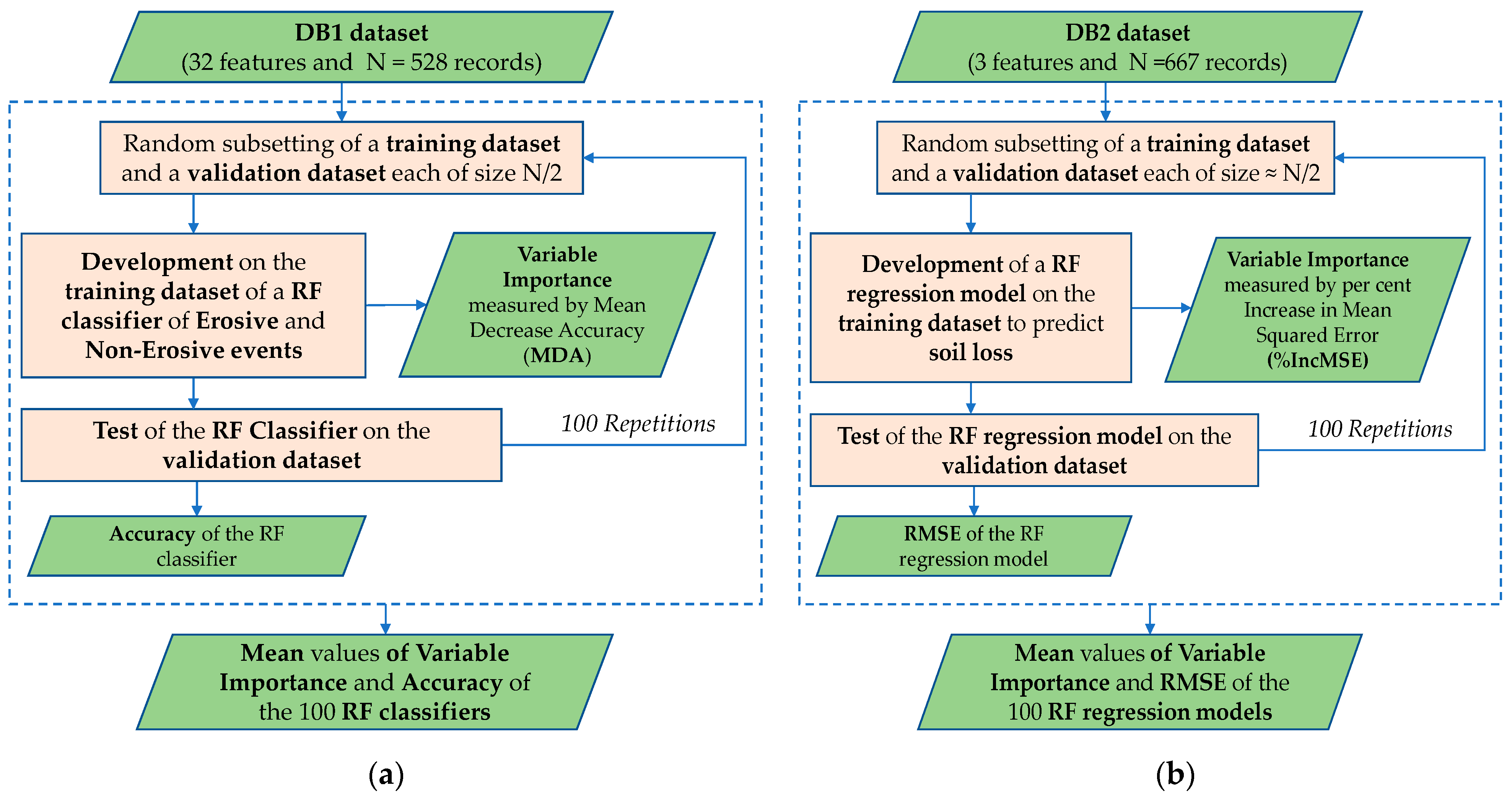
Both UA and PA can be quantified for each category (in this study, for both E and NE rainfall events). A classifier is considered highly accurate when obtaining a combination of high recall and precision values. In particular, high recall (PA) corresponds to a low representation of omission errors and high precision (UA) to a low value of commission errors [42]. In previous works based on different classification techniques [17] other indicators had been used among the performance measures, including the Correct Selection Index (CSI), which is mathematically identical to the PA_E and the Wrong Selection Index (WSI), which is mathematically equal to 1-UA_E. Figure 2a shows the steps carried out to develop and assess the RF classifier.

2.3.2. Random Forest Regression to Predict Event Soil Loss

The initial dataset (DB2) included 667 records. The A_e,N variable is the response variable, and the features considered were Q_R, R, and the period of occurrence of the erosive event, defined as illustrated in Section 2.3.1. The initial dataset was randomly split into 50% for training and 50% for validation. The number of features at each split and the number of trees were set to 2 and 5000, respectively, based on the same preliminary tunings described in Section 2.3.1. The relative importance of a generic feature j was evaluated by quantifying the corresponding average per cent increase in mean squared error (%IncMSE). The %IncMSE of a specific feature in a particular tree is computed as:

$${\%IncMSE}_j=\frac{\left({MSE}_j-MSE0\right)}{MSE0}$$

(7)

where MSE0 is the MSE of that tree in the OOB dataset, and MSE_j is the MSE in the same OOB dataset after the permutation of the feature j. The features with higher %IncMSE are relatively more important than the others for the accuracy of the model prediction. Figure 2b shows the steps carried out to develop and assess the RF regression model.

3. Results

3.1. RF Classifier of Erosive and Non-Erosive Events

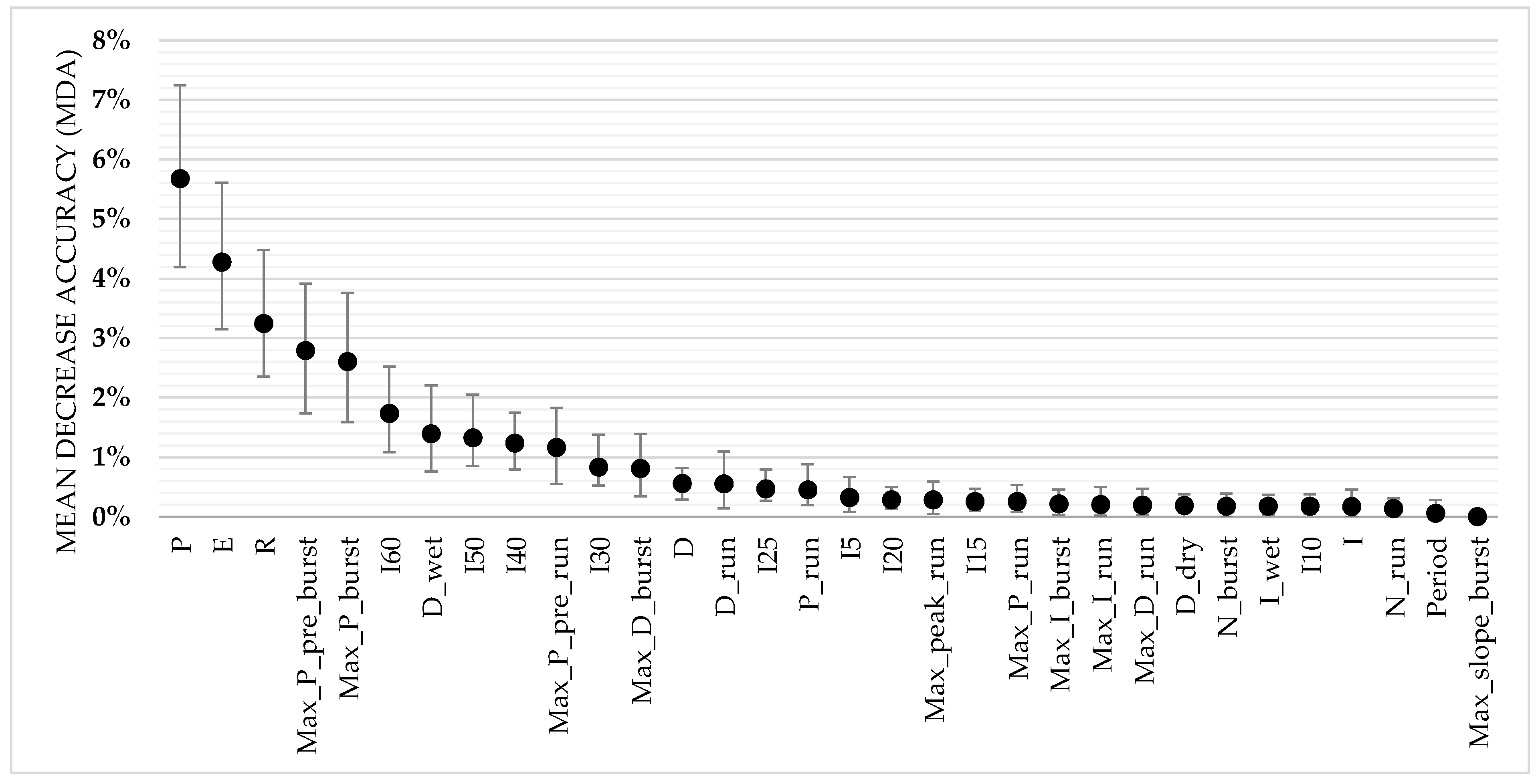
As explained, the RF classifier was trained on a random 50% of the DB1 dataset and then applied to the remaining validation dataset. Since the results depend on the specific observations included in the random training and validation datasets, this procedure was repeated 100 times (Figure 2) to enable a more general and objective assessment. The average feature importance, based on the MDA criterion, is presented in Figure 3.

From Figure 3, six features are found with decidedly higher relative importance than the other variables: the total precipitation P, the kinetic energy E, the erosivity R, the maximum rainfall depth from the start of the event to a burst Max_P_pre_burst, the maximum rainfall amount in a burst Max_P_burst, the maximum intensity over 60 min I60. The “period” feature does not seem helpful for the RF classifier.

The results shown in Figure 4 (dark blue bars) indicate the following accuracy measures: OA 84.8%, PA_E 72.3%, PA_NE 91.0% UA_E 79.2% and UA_NE 87.2%. For comparison purposes, Figure 4 also shows the accuracy values (light blue bars) obtained with a dataset reduced to the 6 top features based on the ranking given Figure 3. It is evident that there is only a slight reduction in the accuracy performances.

3.2. RF Regression Model for Prediction of Event Soil Loss

The RF regression model has been trained on a random 50% of the DB2 (training dataset) and then applied to predict the soil loss A_e,N on the remaining data (validation dataset). For comparison purposes, the same datasets were used to parameterize and validate the USLE_MM model of Equation (3). Since the model performances vary according to the random datasets, this procedure has been repeated 100 times (Figure 2) in order to have a more global and objective evaluation. As for the RF regression model, the variable importance indicates the predominant role of Q_R (mean %IncMSE = 30.2%, CV = 19%) followed by R (%IncMSE = 6.8%, CV = 25%) and the “Period” (%IncMSE = 5.5%, CV = 24%). The average root mean square error (RMSE) of the RF regression model is 2.30 Mg ha⁻¹ (CV = 11%).

The fitting of the USLE_MM model of Equation (3) on the 100 random validation datasets did not lead to a relevant variability in the model parameters (b1 and K_UMM): the average values of b1 and K_UMM are 1.067 and 0.081 with CV of 1.9% and 5.0%, respectively, and they are nearly equal to those obtained on the whole 667-record dataset. Moreover, these values are aligned with those determined in the previous SERLAB 532-record dataset (b1 = 1.0479, K_UMM = 0.0896, [4]) and even with those recently estimated from a small SERLAB 47-record dataset (b1 = 1.10, K_UMM = 0.032, [16]). This indicates that the SERLAB dataset has now reached a size that makes it relatively stable to new data and subsetting. The performance of the USLE_MM model is decidedly lower than the RF regression model, with an average RMSE of 3.34 Mg ha⁻¹ (CV = 9%).

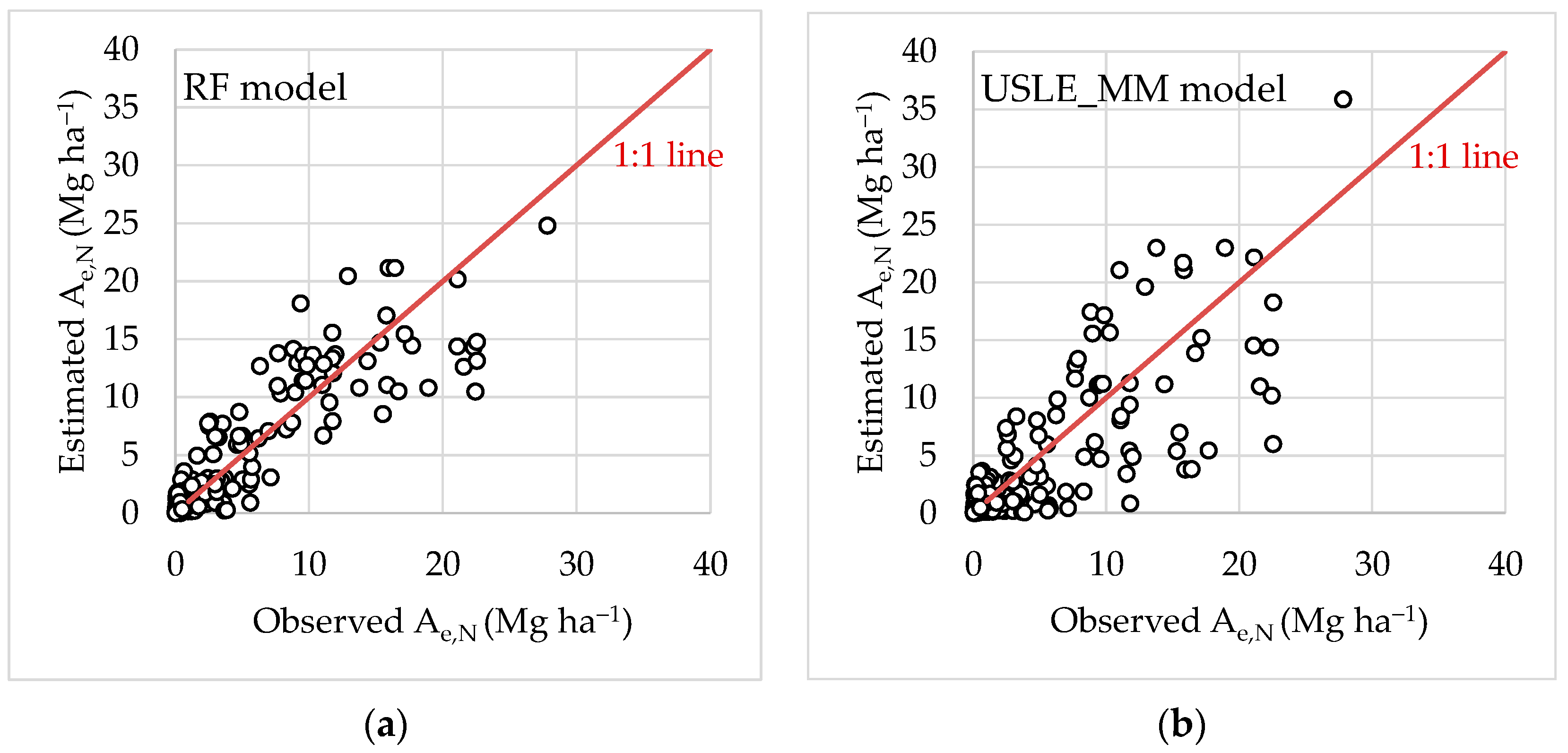
A graphical comparison of the performance of the two models is presented in Figure 5, which shows the scatter plots of observed (x-axis) and predicted (y-axis) A_e,N against the 1:1 line for 1 of the 100 random training/validation datasets.

4. Discussion

The analysis demonstrates that an RF algorithm can be remarkably effective for classifying NE and E storm events based on rainfall characteristics alone. Regarding the variable importance, the results (Figure 3) are consistent with those of previous studies, particularly with those of Todisco et al. [17], which indicated P, R, E, P_max_burst and I60 among the best variables. The importance of the rainfall depth P is also confirmed, as initially proposed by Wischmeier and Smith [5]. The accuracy measures of the classifier (Figure 4) are satisfactory, especially considering that the evaluation refers to a part of the dataset not used for the model training. The most critical accuracy value is the PA_E (72.3%), i.e., the percentage of erosive events correctly recognized to the observed total. Conversely, when the model assigns the “erosive” category to an event, it has a higher success rate (UA_E = 79.2%). These percentages decrease slightly when the model works with the six most significant features (PA_E = 70.0% and UA_E = 76.1%).

The RF classifier appears to be a valid alternative compared to other techniques previously used for the same purpose and on the same dataset. In Todisco et al.’s work [17], the best results (obtained by applying compound rainfall thresholds) indicate higher PA_E (about 82–85%) but lower UA_E (about 72–74%). Furthermore, in that case, the methodology for identifying the thresholds to separate NE and E events had not been made considering the separation between training and validation datasets.

The underestimation of the number of erosive events by the RF classifier does not significantly affect the estimation of the long-term erosivity of rainfall. In fact, the events correctly classified as erosive represent about 91% of the erosivity of all erosive events. This happens because, as known [10,11], the total erosivity is largely due to a few particularly intense or long-lasting storm events that are correctly identified by the RF classifier. The model could therefore be applied in real-time or on past time series to obtain an almost correct identification of the occurrence of the most significant erosion events. Indeed, although it is possible to analyse the variable importance, it is not straightforward to understand how the RF classifier uses the variables (and the corresponding thresholds) to arrive at the final classification.

The RF regression model, developed on only three features (Q_R, R, and “Period”), demonstrates decidedly superior performances (average RMSE = 2.30 Mg ha⁻¹) compared to the traditional USLE_MM power relationship (average RMSE = 3.34 Mg ha⁻¹) tested on the same datasets. This difference can depend on several factors. The first is undoubtedly attributable to the fact that, unlike the USLE_MM, the RF model uses the supplementary explanatory nominal variable “Period”. This feature, useless in the classification algorithms (Figure 3), here proves to be relevant, with importance only slightly lower than the erosivity factor R. As further proof of its importance, an RF regression model, trained only on the Q_R and R features, led to a significant increase in the average RMSE (2.67 Mg ha⁻¹), which is, however, still lower than that of the USLE_MM. The interpretation of the reason of why a simple variable such as the “period” (with only two modes “wet” and “dry”) can improve the soil loss prediction is not accessible, especially in such a type of “black box” model. An influence of the season on the reliability of soil loss prediction models has already been observed by Todisco et al. [43], which attributed this to the different conditions of the soil surface. The climatic conditions (particularly precipitation and air temperature) roughly described by the variable “period” can affect the dynamics of various soil properties such as roughness [44], infiltration and bulk density [45,46], and hydraulic conductivity [47]. Therefore, even if the RF model already explicitly considers essential features such as Q_R and R, the “period” becomes important to allow the model to evaluate the seasonal variability of their effect on soil loss. Finally, the “period” can directly contribute to describing the soil erodibility dynamics not explicitly considered in the model. Indeed, soil erodibility could vary with the “period” due to different environmental and climatic conditions (e.g., different soil moisture and soil temperature), capable of influencing the soil aggregate stability. This type of effect has been widely demonstrated in the literature, such as in [48,49,50]. Therefore, it would seem that the model’s behaviour is consistent with the physical interpretation of the process.

Even without the “period” variable, the RF model is still superior to the USLE_MM one. This is undoubtedly due to the greater flexibility of RF in the use of input variables. In traditional regression, the independent variables are constrained in a precise functional form. In the case of the USLE_MM, using the product variable Q_RR further reduces the possibility of differentiating the effect of Q_R and R.

5. Conclusions

The random forest approach has proven to be more effective than traditional (i.e., non-machine learning) methods in classifying erosive and non-erosive events and in quantifying soil loss at the event temporal scale and plot spatial scale. In this second application, it is conceivable that further performance improvements could be obtained by developing models with feature sets not constrained in the mathematical form of Equation (1). An interesting perspective of this study will be to compare different machine-learning techniques. In general, the possibility of applying such models still strongly depends on the availability of relatively large datasets. This indicates the need to continue investing in experimental and monitoring activities to increase the databases available in the most diverse environmental conditions and make machine learning approaches even more efficient.

References

1. Pimentel, D. Soil erosion: A food and environmental threat. Environ. Dev. Sustain. 2006, 8, 119–137. [Google Scholar] [CrossRef]
2. Borrelli, P.; Van Oost, K.; Meusburger, K.; Alewell, C.; Lugato, E.; Panagos, P. A step towards a holistic assessment of soil degradation in Europe: Coupling on-site erosion with sediment transfer and carbon fluxes. Environ. Res. 2018, 161, 291–298. [Google Scholar] [CrossRef] [PubMed]
3. Risse, L.M.; Nearing, M.A.; Nicks, A.D.; Laflen, J.M. Error assessment in the universal soil loss equation. Soil Sci. Soc. Am. J. 1993, 57, 825–833. [Google Scholar] [CrossRef]
4. Bagarello, V.; Ferro, V.; Pampalone, V.; Porto, P.; Todisco, F.; Vergni, L. Statistical check of USLE-M and USLE-MM to predict bare plot soil loss in two Italian environments. Land Degrad. Dev. 2018, 29, 2614–2628. [Google Scholar] [CrossRef]
5. Wischmeier, W.H.; Smith, D.D. Predicting Rainfall-Erosion Losses: A Guide to Conservation Farming; U.S. Department of Agriculture, Science and Education Administration: Washington, DC, USA, 1978; p. 537.
6. Renard, K.G.; Foster, G.R.; Weesies, G.A.; McCool, D.K.; Yoder, D.C. Predicting soil erosion by water: A guide to conservation planning with the revised universal soil loss equation (RUSLE). In U.S. Department of Agriculture Agricultural Handbook. No. 703; US Department of Agriculture: Washington, DC, USA, 1997. [Google Scholar]
7. Zhou, P.; Luukkanen, O.; Tokola, T.; Nieminen, J. Effect of vegetation cover on soil erosion in a mountainous watershed. Catena 2008, 75, 319–325. [Google Scholar] [CrossRef]
8. Morgan, R.P.C. Soil Erosion and Conservation, 3rd ed.; Blackwell: Malden, MA, USA, 2005; p. 320. [Google Scholar]
9. Larson, W.E.; Lindstrom, M.J.; Schumacher, T.E. The role of severe storms in soil erosion: A problem needing consideration. J. Soil Water Conserv. 1997, 52, 90–95. [Google Scholar]
10. Bagarello, V.; Ferro, V.; Pampalone, V.; Porto, P.; Todisco, F.; Vergni, L. Predicting soil loss in central and south Italy with a single USLE-MM model. J. Soils Sediments 2018, 18, 3365–3377. [Google Scholar] [CrossRef]
11. Di Stefano, C.; Pampalone, V.; Todisco, F.; Vergni, L.; Ferro, V. Testing the Universal Soil Loss Equation-MB equation in plots in Central and South Italy. Hydrol. Process. 2019, 33, 2422–2433. [Google Scholar] [CrossRef]
12. Kinnell, P.I.A.; Risse, L.M. USLE-M: Soil Empirical modeling rainfall erosion through runoff and sediment concentration. Sci. Soc. Am. J. 1998, 62, 1667–1672. [Google Scholar] [CrossRef]
13. Kinnell, P.I.A. Event soil loss, runoff and the Universal Soil Loss Equation family of models: A review. J. Hydrol. 2010, 385, 384–397. [Google Scholar] [CrossRef]
14. Bagarello, V.; Di Piazza, G.V.; Ferro, V.; Giordano, G. Predicting unit plot soil loss in Sicily, south Italy. Hydrol. Process. 2008, 22, 586–595. [Google Scholar] [CrossRef]
15. Bagarello, V.; Ferro, V.; Pampalone, V. A new version of the USLEMM for predicting bare plot soil loss at the Sparacia (South Italy) experimental site. Hydrol. Process. 2015, 29, 4210–4219. [Google Scholar] [CrossRef]
16. Todisco, F.; Vergni, L.; Ortenzi, S.; Di Matteo, L. Soil Loss Estimation Coupling a Modified USLE Model with a Runoff Correction Factor Based on Rainfall and Satellite Soil Moisture Data. Water 2022, 14, 2081. [Google Scholar] [CrossRef]
17. Todisco, F.; Vergni, L.; Vinci, A.; Pampalone, V. Practical thresholds to distinguish erosive and rill rainfall events. J. Hydrol. 2019, 579, 124173. [Google Scholar] [CrossRef]
18. Xie, Y.; Liu, B.; Nearing, M.A. Practical thresholds for separating erosive and non-erosive storms. Trans. Am. Soc. Agric. Eng. 2002, 45, 1843–1847. [Google Scholar]
19. Todisco, F. The internal structure of erosive and non-erosive storm events for interpretation of erosive processes and rainfall simulation. J. Hydrol. 2014, 519, 3651–3663. [Google Scholar] [CrossRef]
20. Mukhamediev, R.I.; Popova, Y.; Kuchin, Y.; Zaitseva, E.; Kalimoldayev, A.; Symagulov, A.; Levashenko, V.; Abdoldina, F.; Gopejenko, V.; Yakunin, K.; et al. Review of Artificial Intelligence and Machine Learning Technologies: Classification, Restrictions, Opportunities and Challenges. Mathematics 2022, 10, 2552. [Google Scholar] [CrossRef]
21. Licznar, P.; Nearing, M.A. Artificial Neural Networks of Soil Erosion and Runoff Prediction at the Plot Scale. Catena 2003, 51, 89–114. [Google Scholar] [CrossRef]
22. Kim, M.; Gilley, J.E. Artificial Neural Network Estimation of Soil Erosion and Nutrient Concentrations in Runoff from Land Application Areas. Comput. Electron. Agric. 2008, 64, 268–275. [Google Scholar] [CrossRef] [Green Version]
23. Albaradeyia, I.; Hani, A.; Shahrour, I. WEPP and ANN Models for Simulating Soil Loss and Runoff in a Semi-Arid Mediterranean Region. Environ. Monit. Assess. 2011, 180, 537–556. [Google Scholar] [CrossRef]
24. de Farias, C.A.S.; Santos, C.A.G. The Use of Kohonen Neural Networks for Runoff–Erosion Modeling. J. Soils Sediments 2014, 14, 1242–1250. [Google Scholar] [CrossRef]
25. Arif, N.; Danoedoro, P. Hartono Analysis of Artificial Neural Network in Erosion Modeling: A Case Study of Serang Watershed. IOP Conf. Ser. Earth Environ. Sci. 2017, 98, 012027. [Google Scholar] [CrossRef] [Green Version]
26. Yusof, M.F.; Azamathulla, H.M.; Abdullah, R. Prediction of Soil Erodibility Factor for Peninsular Malaysia Soil Series Using ANN. Neural Comput. Appl. 2014, 24, 383–389. [Google Scholar] [CrossRef]
27. Breiman, L. Random forests. Mach. Learn. 2001, 45, 5–32. [Google Scholar] [CrossRef] [Green Version]
28. Wang, S.; Aggarwal, C.; Liu, H. Random-Forest-Inspired Neural Networks. ACM Trans. Intell. Syst. Technol. 2018, 9, 69. [Google Scholar] [CrossRef] [Green Version]
29. Tyralis, H.; Papacharalampous, G.; Langousis, A. A Brief Review of Random Forests for Water Scientists and Practitioners and Their Recent History in Water Resources. Water 2019, 11, 910. [Google Scholar] [CrossRef] [Green Version]
30. Konstantinou, C.; Stoianov, I. A comparative study of statistical and machine learning methods to infer causes of pipe breaks in water supply networks. Urban Water J. 2020, 17, 534–548. [Google Scholar] [CrossRef]
31. Konstantinou, C.; Biscontin, G. Experimental Investigation of the Effects of Porosity, Hydraulic Conductivity, Strength, and Flow Rate on Fluid Flow in Weakly Cemented Bio-Treated Sands. Hydrology 2022, 9, 190. [Google Scholar] [CrossRef]
32. Schoppa, L.; Disse, M.; Bachmair, S. Evaluating the performance of random forest for large-scale flood discharge simulation. J. Hydrol. 2020, 590, 125531. [Google Scholar] [CrossRef]
33. Park, H.; Kim, K.; Lee, D.K. Prediction of Severe Drought Area Based on Random Forest: Using Satellite Image and Topography Data. Water 2019, 11, 705. [Google Scholar] [CrossRef] [Green Version]
34. Tarek, Z.; Elshewey, A.M.; Shohieb, S.M.; Elhady, A.M.; El-Attar, N.E.; Elseuofi, S.; Shams, M.Y. Soil Erosion Status Prediction Using a Novel Random Forest Model Optimized by Random Search Method. Sustainability 2023, 15, 7114. [Google Scholar] [CrossRef]
35. Todisco, F.; Vergni, L.; Mannocchi, F.; Bomba, C. Calibration of the soil loss measurement method at the Masse experimental station. Catena 2012, 91, 4–9. [Google Scholar] [CrossRef]
36. Vergni, L.; Vinci, A.; Todisco, F. Influence of the rainfall Time Step on the Thresholds for Separating Erosive and Non-Erosive Events. In AIIA 2022: Biosystems Engineering towards the Green Deal; Lecture Notes in Civil Engineering; Ferro, V., Giordano, G., Orlando, S., Vallone, M., Cascone, G., Porto, S.M.C., Eds.; Springer Nature: Berlin, Germany, 2023; Volume 337, in press. [Google Scholar]
37. Nearing, M.A. A single continuous function for slope steepness influence on soil loss. Soil Sci. Soc. Am. J. 1997, 61, 917–919. [Google Scholar] [CrossRef]
38. Vinci, A.; Todisco, F.; Mannocchi, F. Calibration of manual measurements of rills using terrestrial laser scanning. Catena 2016, 140, 164–168. [Google Scholar] [CrossRef]
39. Liaw, A.; Wiener, M. Classification and Regression by random Forest. R News 2002, 2–3, 18–22. [Google Scholar]
40. Breiman, L. Manual on Setting up, Using, and Understanding Random Forests v3.1; Statistics Department University of California: Berkeley, CA, USA, 2002; pp. 1–58. [Google Scholar]
41. Congalton, R.G. A review of assessing the accuracy of classifications of remotely sensed data. Remote Sens. Environ. 1991, 37, 35–46. [Google Scholar] [CrossRef]
42. Weaver, J.; Moore, B.; Reith, A.; McKee, J.; Lunga, D. A comparison of machine learning techniques to extract human settlements from high resolution imagery. In Proceedings of the International Geoscience and Remote Sensing Symposium (IGARSS), Valencia, Spain, 22–27 July 2018. [Google Scholar]
43. Todisco, F.; Brocca, L.; Termite, L.F.; Wagner, W. Use of satellite and modeled soil moisture data for predicting event soil loss at plot scale. Hydrol. Earth Syst. Sci. 2015, 19, 3845–3856. [Google Scholar] [CrossRef] [Green Version]
44. Vinci, A.; Todisco, F.; Vergni, L.; Torri, D. A comparative evaluation of random roughness indices by rainfall simulator and photogrammetry. Catena 2020, 188, 104468. [Google Scholar] [CrossRef]
45. Todisco, F.; Vergni, L.; Vinci, A.; Torri, D. Infiltration and bulk density dynamics with simulated rainfall sequences. Catena 2022, 218, 106542. [Google Scholar] [CrossRef]
46. Todisco, F.; Vergni, L.; Ceppitelli, R. Modelling the dynamics of seal formation and pore clogging in the soil and its effect on infiltration using membrane fouling models. J. Hydrol. 2023, 618, 129208. [Google Scholar] [CrossRef]
47. Todisco, F.; Vergni, L.; Iovino, M.; Bagarello, V. Changes in soil hydrodynamic parameters during intermittent rainfall following tillage. Catena 2023, 226, 107066. [Google Scholar] [CrossRef]
48. Torri, D.; Ciampalini, R.; Gil, P.A. The Role of Soil Aggregates in Soil Erosion Processes. In Modelling Soil Erosion by Water; Boardman, J., Favis-Mortlock, D., Eds.; NATO ASI Series; Springer: Berlin/Heidelberg, Germany, 1998; Volume 55, pp. 247–257. [Google Scholar]
49. Lavee, H.; Sarah, P.; Imeson, A.C. Aggregate Stability Dynamics as Affected by Soil Temperature and Moisture Regimes. Geogr. Ann. A 1996, 78, 73–82. [Google Scholar]
50. Imeson, A.C.; Lavee, H.; Calvo, A.; Cerda, A. The erosional response of calcareous soils along a climatological gradient in Southeast Spain. Geomorphology 1998, 24, 3–16. [Google Scholar] [CrossRef]
Figure 1. The SERLAB experimental site for soil loss monitoring at plot scale: (a) pan view; (b) meteorological station; (c) detail of the storage tanks.
Water 15 02225 g001
Figure 2. Workflow of the analyses carried out for the development and assessment of (a) an RF classifier of erosive and non-erosive rainfall events; (b) an RF regression model to predict the event soil loss at the plot spatial scale.
Water 15 02225 g002
Figure 3. Importance of the features considered in the RF classifier, based on the mean decrease accuracy (MDA) criterion. Black dots and grey bars represent the mean and 90% confidence interval of the MDA values obtained in 100 random repetitions. The definition of the variables is given in Table A1.
Water 15 02225 g003
Figure 4. Mean accuracy measures of RF classifiers trained on the original dataset (32 features) and on the top 6 variables (based on the Mean Decrease Accuracy criterion, Figure 3). OA = Overall Accuracy; UA = User Accuracy; PA = Producer Accuracy; E = Erosive events; NE: Non-erosive events. Mean values obtained from 100 training and validation datasets.
Water 15 02225 g004
Figure 5. Comparison between observed and estimated normalized soil loss Ae,N obtained using (a) the RF regression model; (b) the USLE mm regression model. Both models are trained on the same random 50% dataset and then applied to the remaining data.
Water 15 02225 g005