Article

Driving Factors of the Hydrological Response of a Tropical Watershed: The Ankavia River Basin in Madagascar

by
Zonirina Ramahaimandimby
1,*,
Alain Randriamaherisoa
2,
Marnik Vanclooster
1 and
Charles L. Bielders
1
1
Earth and Life Institute, Université Catholique de Louvain, 1348 Ottignies-Louvain-la-Neuve, Belgium
2
Civil Engineering Department, Université d’Antananarivo, Antananarivo 101, Madagascar
*
Author to whom correspondence should be addressed.
Water 2023, 15(12), 2237; https://doi.org/10.3390/w15122237
Submission received: 28 April 2023 / Revised: 30 May 2023 / Accepted: 5 June 2023 / Published: 14 June 2023
(This article belongs to the Topic Hydrology and Water Resources Management)

Abstract

:
Understanding the hydrological behavior of watersheds (WS) and their driving factors is crucial for sustainable water resources management. However, at large scales, this task remains challenging due to the spatial heterogeneity in landscapes, topography and morphology (T), land cover (LC), geology (G), and soil properties (S). In this context, the aim of this study was to identify the key factors that influence the hydrological signatures of four watersheds: Ankavia (WS1: 55% forest cover), Ankaviabe (WS2: 77% forest cover), Sahafihitry (WS3: 41% forest cover), and Antsahovy (WS4: 48% forest cover), over a 10-month study period. These catchments are located within the SAVA region of northeastern Madagascar and have a humid tropical climate. We investigated the relationship between selected catchment descriptors and hydrological signatures by using a Pearson coefficient-based correlation matrix. More specifically, catchment descriptors (extracted from T, LC, G, and S) were correlated with the following hydrological signatures: base flow index (BFI), mean runoff coefficient (rc), mean peak flow (Qp), mean runoff event time scales (ts), high flows (Q5), low flows (Q95), and mean discharge (q_mean). The analysis revealed that land cover, soil properties, and geology seem to be the best predictors for BFI and Q95, while soil properties mainly govern rc, Qp, Q5, ts, and q_mean. These findings provide valuable insights into the key drivers of hydrological behavior that can inform water resource management strategies. In particular, WS2 exhibits better flood buffering capacity but also experiences lower base flows in the dry season, potentially due to higher evapotranspiration. Conversely, WS3 and WS4 (and to a lesser extent WS1) have lower flood buffering capacity, but these watersheds encounter less pronounced low flows in the dry season due to higher BFIs, possibly attributable to lower evapotranspiration rates. The results underscore the importance of responsible land use practices and conservation efforts, which are essential for the sustainable development of the region. By incorporating these practices into water management strategies, we can help ensure a more stable and reliable water supply for communities and ecosystems within the region.

1. Introduction

Global changes, such as population growth, industrial development, agricultural expansion, and climate change, are exerting strong pressures on natural resources in general, and on water resources in particular [1,2,3]. In turn, the resulting stresses on water resources are having a significant impact on production, economic growth, health, livelihoods, and national security [4]. As a result, achieving sustainable management of water resources is a pressing issue, and it will be even more so in the future.
In order to support the sustainable use of water in the face of socio-economic and environmental constraints, understanding the impact of global changes on hydrology is essential [5,6]. This includes an in-depth understanding of the physical drivers of the hydrological response over time and space within the regions to be managed [7]. As water management is often operated across large areas, this represents a significant challenge considering the complex interactions of natural and human processes that may operate concurrently and affect the spatial and temporal variability of the water system [8,9]. This is particularly true in large tropical watersheds because of the rapid pace at which these processes change in response to the growing population pressure, economic development, and climate change. Furthermore, local economies and livelihoods across much of the tropics heavily rely on water availability [10], while the limited economic and development capabilities enhance water-related risks (limitations in water supply, floods, and droughts), making countries from the Global South among the most vulnerable to climate change impacts [11].
Most of our current understandings of hydrological responses are derived from small-scale catchment studies [12,13]. However, in tropical areas, the study of watershed behavior at a small- and meso-scale remains problematic due to a lack of monitoring infrastructure [14,15,16]. As a result, in recent decades, most efforts in tropical areas have been invested in studies of large watersheds rather than small-scale or meso-scale catchments [17,18]. However, large tropical watersheds may be composed of a wide variety of soil types, geological formations, and land covers, making the scaling of hydrological behavior problematic and resulting sometimes in conflicting results [19]. Indeed, whereas some studies conducted in tropical areas have reported considerable hydrological alterations in response to land cover changes in large watersheds [20,21,22], others have shown that the influence of changing forest cover on river hydrology was insignificant [23,24,25]. These inconsistencies may be related to the specificities of the study sites, but also to the large scale of the study of the watersheds and the resulting complexity [22]. More studies at the small- and meso-scale are thus needed to help better understand the hydrological behavior of tropical watersheds. Besides, the challenge to understand catchment response at smaller scales to changing environmental conditions in tropical regions is still very much a topical issue since many climate mitigation strategies are implemented at these smaller scales [7,26].
Madagascar—a tropical island state in southern Africa—is faced with various water-related management issues [27,28,29]. About 80% of the active population’s livelihoods, including agriculture, livestock farming, fishing, and fluvial transportation, are water dependent [27]. The impacts of global changes on hydrology have already been observed, particularly due to the location of the country in the Indian Ocean and its 5000 km coastline, which makes the island extremely vulnerable to climate change and extreme events [30,31]. Floods often occur in northern and central areas, while droughts are recurrent in certain southern regions [28,31]. Over the past decades, to cater to the growing population needs, a significant amount of rainforest cover has been converted into a mosaic of land uses representing various stages of the swidden farming cycle, including severely degraded grasslands [17,32]. Such changes can potentially affect the soil infiltration capacity, leading to increased surface runoff and peak discharge of rivers [33,34]. Unfortunately, the country has very few monitored watersheds, which is a prerequisite to better understanding the hydrological functioning at different scales and designing sustainable water and land use management strategies. Also, creating a credible database for hydrological studies is jeopardized by the highly incomplete and dispersed data from the national weather service stations [31,35].
As a contribution to filling this current knowledge gap, this study aimed to identify the key factors governing hydrological response at the meso-scale using the humid tropical Ankavia catchment in Madagascar as a case study. The data collected will be used in a recently installed rainfall and discharge monitoring network. To reach this overall objective, we address the following specific objectives: (i) to document the Ankavia catchment characteristics; (ii) to analyze the hydrological responses in the catchment; and (iii) to identify the groups of factors (topographic, morphometric, pedo-geological, and land cover properties) that are the most informative to understand these hydrological responses. The study should serve as a basis for the future implementation of an Integrated Water Resources Management (IWRM) system in the SAVA region (northeastern Madagascar).

2. Materials and Methods
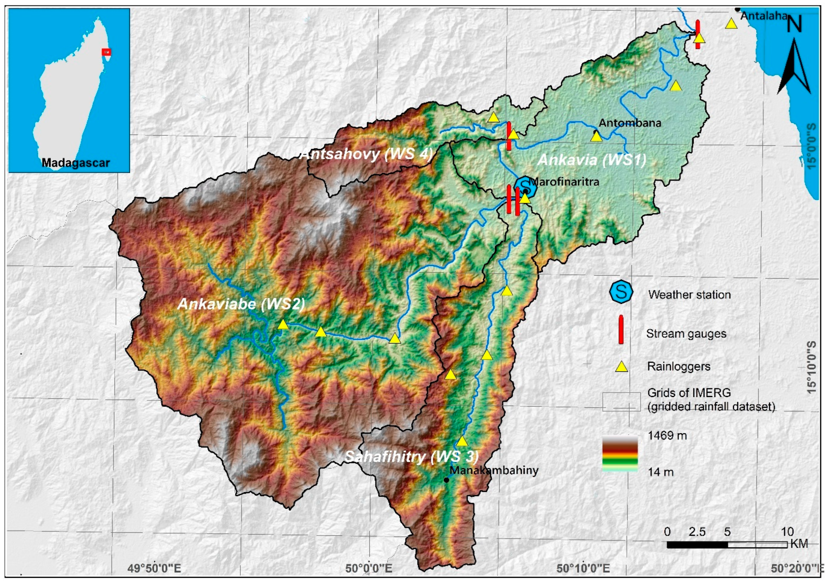
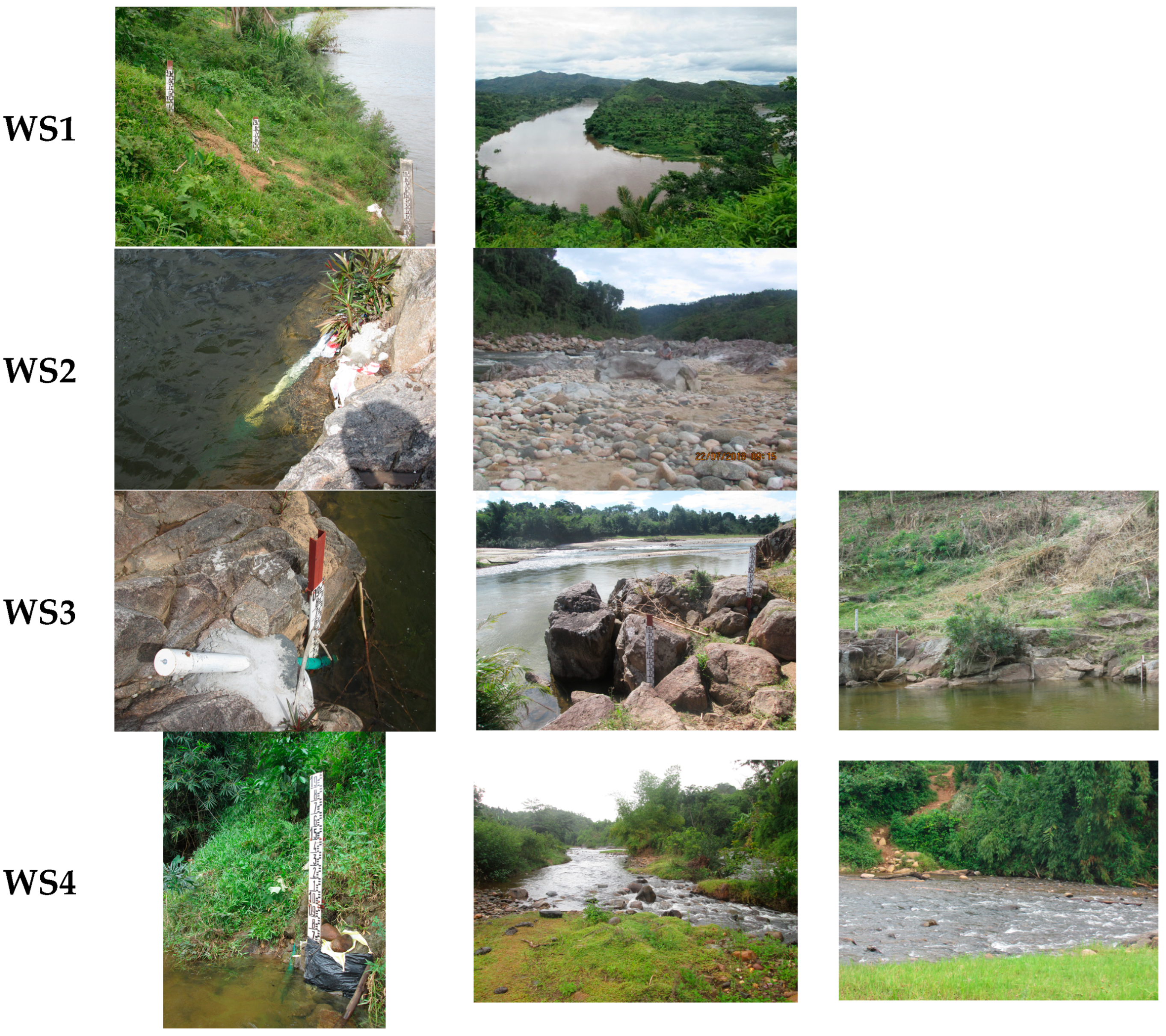
2.1. Study Area

The Ankavia watershed (WS1) is situated in the district of Antalaha, a city in the SAVA (Sambava–Andapa–Vohémar–Antalaha) region of northeastern Madagascar (Figure 1). It covers an area of 1116 km2 and 55% of the basin is occupied by forest. The watershed lies between 14°90′ and 15°20′ South Latitude and between 49°45′ and 50°15′ East Longitude. The Ankavia river is formed by three tributaries before flowing into the Ankavanana river, which reaches the Indian Ocean. The three upstream sub-catchments are Ankaviabe (WS2; 624 km2; 77% forest cover), Sahafihitry (WS3; 197 km2; 41% forest cover), and Antsahovy (WS4; 70 km2; 48% forest cover). The basin has a total length of 54.6 km, and its elevation varies from 14 m a.m.s.l. at the outlet to 1469 m a.m.s.l. at the highest point on the escarpment (Figure 1). For the purpose of this study, the outlet of the Ankavia was located at the Antsahamanenona Drinking Water Supply Station of Antalaha, which provides drinking water for the city’s 280,000 inhabitants [36]. Additionally, the water-related stresses experienced in the Ankavia basin are similar to those experienced in other basins in the region [37].
According to the meteorological station in Antalaha, the average annual rainfall in the area is 2241 mm (1960–2017). There is a wet rainy season between December and April, while a dry (but still rainy) season occurs from May to November. The daily maximum temperature of 31.4 °C is observed in January, while the minimum temperature of 18.9 °C is observed in August [38]. The western part of the Ankavia watershed is dominated by primary forests, while the eastern part is occupied by a mosaic of natural vegetation composed of shrubs and herbaceous cover [38].
The geology of Madagascar consists of a patchwork of Precambrian rocks, mainly high-grade metamorphic basement domains overlain by unmetamorphosed sedimentary rocks and poorly weathered low-grade metasediments [39]. In the Antalaha area, two different cover sequences lay on high-grade metamorphic and igneous foundation rocks of the Archaean ‘Antongil’ craton and the Neoproterozoic ‘Bemarivo’ belt. The elder of these two cover sequences, the ‘Andrarona’ Group, is composed of low-grade metasedimentary rocks, while the younger sequence, the ‘Ampohafana’ formation, is made up of unmetamorphosed sedimentary rocks [39]. The pedology of the basin is dominated by Ferrasols upstream and Acrisols downstream [40].

2.2. Watershed Attributes

Several satellite products and thematic maps (Table 1) were used to determine the characteristics of the Ankavia catchment and sub-catchments in terms of topography/morphometry, land cover, soil, and geology (Figure 2). The 30 m digital elevation model (DEM) of the Shuttle Radar Topography Mission (SRTM; [41]) was used to derive the topographic and morphometric attributes (Figure 1). The 2019 land cover of the Ankavia catchment was extracted from GlobCover v2 [42], which has a spatial resolution of 300 m (Figure 2a). The 250 m SoilGRIDs (global gridded soil information) was used to retrieve the soil attributes (Figure 2b), including the organic carbon data at three depths (0–5, 5–15, 15–30 cm), and the dominant soil order based on the World Reference Base (WRB) (Figure 2c) [43]. Hydrologic soil groups were extracted using HYSOGs250m (Figure 2d) [44], which were created to assist with USDA-based (United States Department of Agriculture) curve number runoff modeling at regional and continental scales. The four standard hydrological soil groups (HSG-A, HSG-B, HSG-C, and HSG-D) correspond to soils with increasing levels of runoff potential (low, moderately low, moderately high, and high, respectively). Lastly, the modified geological map (1/100,000 scale) was provided by the Ministry of Energy and Mines through the Mineral Resources Governance Program (PGRM) (Figure 2e).

2.3. Hydrometeorological Datasets

Even though rain gauges were installed as part of the project [45], their spatial coverage was uneven across the watershed, with no gauges in the western part and at the higher altitudes due to accessibility issues (Figure 1). Consequently, the gridded precipitation product IMERG V06 Final was used in the present study [46] (Figure 1). Ref. [45] demonstrated that the IMERG v06 Final data is a reliable alternative to ground-based measurements for event and daily time scales or greater. We used the IMERG product at the event time scale for the time period covered by the discharge measurements, as described below.
To measure the discharge, we installed four gauging stations at the outlet of each catchment (Figure 1). These locations were chosen for their accessibility and the stability of the riverbed sections (predominantly composed of rocks) (Appendix A). Starting on September 2018, all four stations were operational. Water levels were monitored using Solinst® LTC Levelogger Edge M5 C80 pressure sensors (Level measurement device, Solinst Canada Ltd., Georgetown, ON, Canada) with an accuracy of ±0.3 cm. The atmospheric pressure was recorded using a Solinst® sensor 3001 LT Barologger Edge, M1.5/F5, with a precision of ±0.05 kPa located at the climatic station of Marofinaritra (Figure 1).
The data were collected with a 1 h timestep (GMT+ 0). The equipment was checked monthly, and data were regularly checked for consistency and completeness. In this study, we used the hydrometric data collected from September 2018 to June 2019, which is the period during which all 4 gauging stations were operational concurrently. After this period, one or more stations were not operational due to damage by extreme floods or technical issues with the probes.

2.4. Catchment Descriptors (CD) Analysis

A wide range (37 in total) of catchment descriptors representing topography/morphometry (T), land cover (LC), soil properties (S), and geology (G) of the Ankavia catchment were acquired and calculated. Table 2 lists the metadata of catchment descriptors.

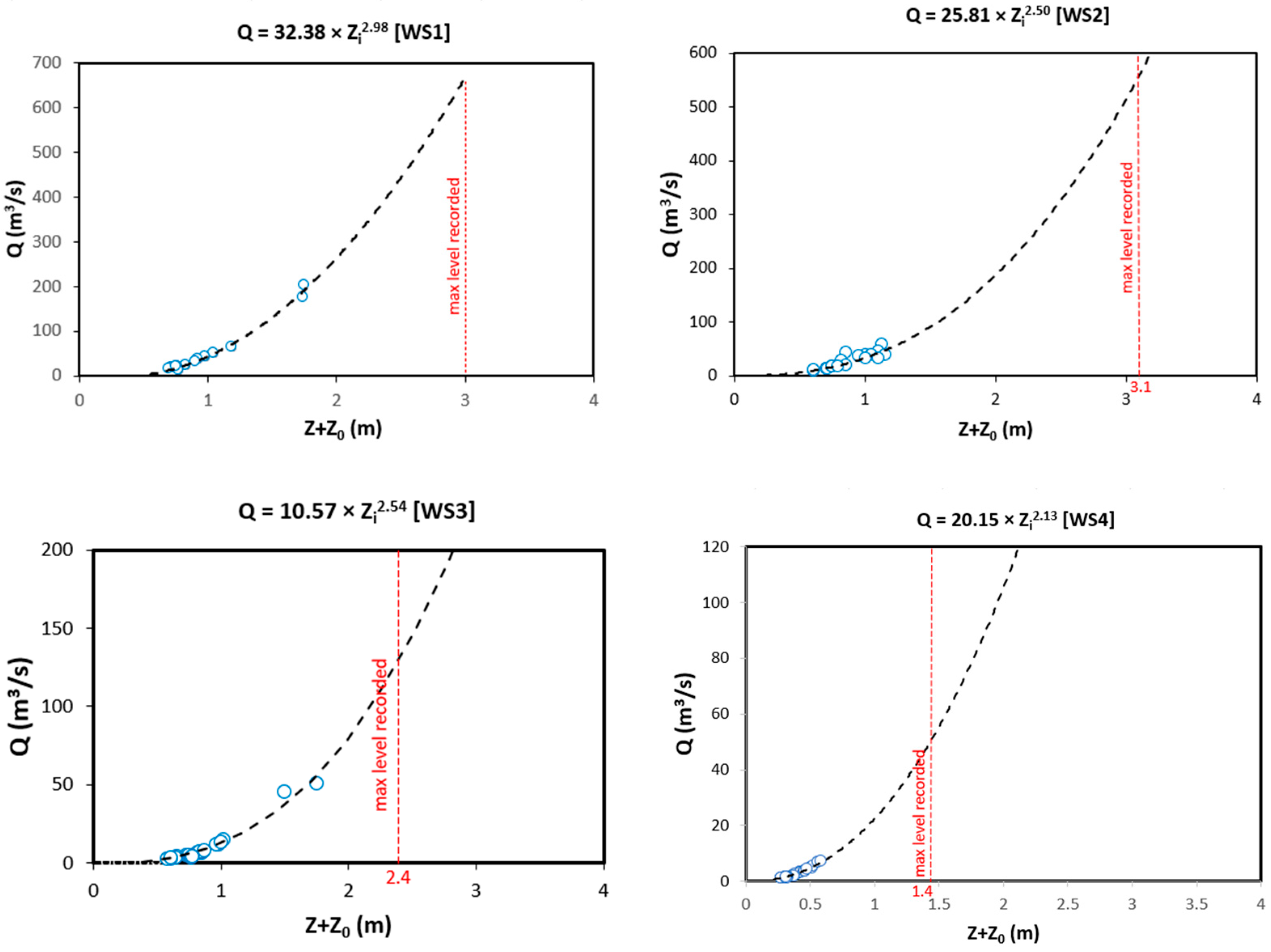
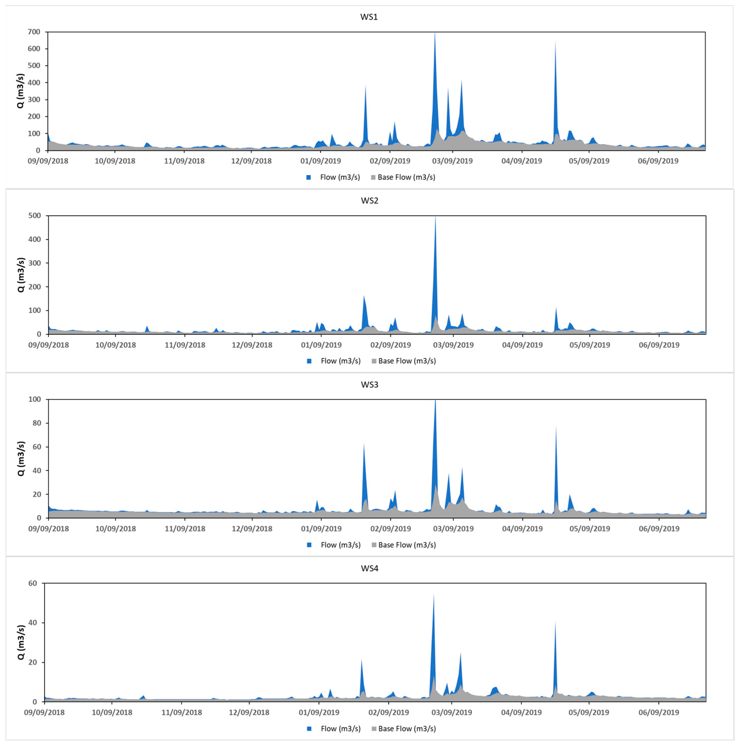
2.5. Streamflow Analysis

At first, since the atmospheric pressure varies with elevation [52], the atmospheric pressure recorded at the Marofinaritra weather station was corrected using Equation (1) for an isothermal atmosphere to provide atmospheric pressure at the outlet of each catchment.
P(hi) = P(h0) × e−Δh/hs,
with hs = R × T/M × g
where: P(hi) is the effective atmospheric pressure at elevation hi [Pa],
P(h0) is the atmospheric pressure measured at the Marofinaritra station at elevation h0 [Pa],
Δh is the difference in elevation between hi and h0,
R is the molar gas constant [8.314 J K−1 mol−1],
T is the absolute temperature of the air, taken at the Marofinaritra station [°K],
M is the average molar mass of gas in the atmosphere [0.02896 kg mol−1],
g is the gravitational acceleration [9.81 m·s−2].
Then, the water level from the Levelogger data was obtained using Equation (2).
Z = (PiP(hi))/ρ × g
where Z represents the water level [m],
Pi is the measured water pressure [Pa] at a given outlet,
P(hi) is the atmospheric pressure [Pa] at each sub-catchment outlet,
and ρ is the density of water (1000 kg/m3).
The discharge was determined by converting water level data time series to discharge through the rating curve equation for each outlet (Appendix B). During flow gauging, water velocity for low and medium flows (Q) was measured using an OTT MF PRO magnetic induction current meter (OTT hydromet GmbH, Kempten, Germany), which has a measuring range of 0 to 6 m·s−1 and an accuracy of ±2% of the measured value ±0.015 m·s−1 (between 0 and 3 m·s−1) and ±4% of the measured value ±0.015 m·s−1 (between 3 and 5 m·s−1). At least 20 gauging operations were carried out at each outlet to establish the rating curve, using the measured pairs of water level and discharge (Qi, Zi) for low and medium flow conditions. Then, a power function (Equation (3)) was fitted to the water level discharge data:
Q = a × (Zi)b
where a and b are fitting coefficients,
Zi = Z + Z0, Z is the water level [m] measured by the Levelogger,
and Z0 is the stage at zero discharge [m].
Due to safety concerns during high flow conditions and practical limitations, the rating curves for high flows were extrapolated by using an empirical method based on Manning’s equation (Equation (4)).
Q = (1/n) × Cs × Hr2/3 × Sl1/2
where n is the roughness coefficient of the channel [s·m−1/3], derived from stream gauging for lower and medium flow conditions by combining Equations (3) and (4), Cs is the cross-sectional area of flow [m2], Hr is the hydraulics radius [m], the ratio of the cross-sectional area of fluid flow to the wetted perimeter, and Sl is the slope of the river (%) at the gauging station, estimated from 30 m resolution DEM.

2.6. Hydrological Signatures (HS) Analysis

Hydrological signatures (HS) are quantitative metrics or indices that define statistical or dynamical properties of hydrologic data series [53]. These signatures can be computed using various data sources but, in practice, they are most often calculated using rainfall-runoff time series. In this study, the HS indicators were derived from rainfall-runoff datasets for the 10-month study period.

2.6.1. Event Identification

Rainfall events were defined as periods of non-zero basin-average rainfall interspersed with periods of zero rainfall, considering a minimum cumulative rainfall amount of 2.5 mm and a minimum inter-event time of 6 h [45].
A runoff event is characterized by a runoff start, peak(s), and end. The start of a direct runoff event was defined as the moment in time closest to the (first) peak when total streamflow equals baseflow (Figure 3). The end is reached as soon as total streamflow falls back to the baseflow level (see further). Rainfall and runoff events were then matched, resulting in three cases: (i) rainfall event without runoff event, (ii) rainfall with runoff event, and (iii) runoff without (measured) rain event. In the study, we took into account only the two first cases.

2.6.2. Hydrograph Separation

The Eckhardt method (Equation (5); [54]) was used to separate the discharge data into quickflow (Qf; the direct flow in response to a rainfall event) and baseflow (Qbf: the delayed flow from storage) (Appendix C). This method relies on two parameters: the filter parameter (k) and the maximum baseflow index (BFImax). The filter parameter, which describes the rate at which the streamflow decreases with time following a recharge event, is estimated through recession analysis, while the BFImax is the maximum value of the baseflow index that can be modeled through the recursive digital filter algorithm [54].
Q b , t = 1 B F I m a x × k × Q b , t 1 + 1 k × B F I m a x × Q s , t 1 k × B F I m a x
where Qb,t and Qb,t−1 are the baseflow at time steps t and t − 1, respectively; Qs,t is the total streamflow at time step t; BFImax refers to maximum baseflow index (ratio of baseflow to the total flow), and k is the filter parameter.
In the present study, we employed the Web-based Hydrograph Analysis Tool (WHAT) [55] to separate baseflow from total streamflow. In Equation (5), baseflow for the first time step, Qb,t−1, was assumed to be 50% of the total streamflow. Ref. [56] proposed different BFImax values for various aquifer types. Based on the hydrological and geological characteristics of the studied watersheds, we considered the catchments to have porous aquifers and perennial streams. Therefore, the default BFImax was set to 0.80 while the filter parameter ‘k’ was optimized through recession analysis of selected events [57].

2.7. Hydrological Signatures Analysis

A large number of hydrological signatures (HS) have been proposed in the literature but there are some general selection criteria. According to [58], HS should meet the following requirements: (i) they can be related to hydrological processes to better understand catchment behavior; (ii) they are sensitive to events occurring over different time periods; and (iii) they are not redundant. Based on these criteria, this study used the following HSs: baseflow index (BFI); runoff coefficient (rc); peak discharge (Qp); runoff event time scale (ts); high flows (Q5); low flows (Q95); and mean discharge (q_mean) (Table 3).
BFI is the ratio of total baseflow to total discharge during the observation period. Runoff coefficient rc is the ratio of the quickflow volume of a specific runoff event to the corresponding rainfall. The peak discharge, Qp, represents the maximum rate of discharge during the period of runoff resulting from a rainfall event. The time scale ts is the ratio between quickflow volume and the peak discharge of a specific runoff event. It is an indicator of catchment flashiness and a measure of the importance of fast runoff generation processes, such as overland flow or fast subsurface storm flow. Fast-reacting catchments will have small ts, while catchments with slower runoff generation processes tend to have larger ts. In this study, ts is normalized by the length of the main river. Rc, Qp, and ts were determined for each individual event. Q5 and Q95 were derived from the flow duration curves (FDC), which are cumulative frequency curves that show the percentage of the time that a specified discharge is equaled or exceeded during a given period [59]. The FDC combines the flow characteristics of a stream throughout the range of observed discharges, without regard to the sequence of occurrence. Q5 (the 5th percentile of flow) and Q95 (the 95th percentile) correspond to the discharge that equaled or exceeded 5% (high flows) or 95% (low flows) of the time, respectively. Finally, q_mean is the mean daily discharge during the 10-month study period.
Table 3. Hydrological signatures of runoff events used in the present study.
HS (Unit)DescriptionsCalculationReferences
BFI (-)Ratio of total baseflow (Qbf) to total discharge (Q) during the observation period; hydrograph separation performed according to [55].BFI = Q b f Q [55]
rc (mm/mm)The ratio of the quickflow volume (Qf) of a specific runoff event [mm] to the corresponding rainfall (Ri). Mean of all events [mm].rc = Q f R i [60]
Qp (mm/h)Highest value of the discharge during an event (mean value). [61]
ts (h/km)Ratio between quickflow volume (Qf) [mm] and the peak discharge (Qp) [mm/h] multiplied by the length of the main river (Lc) [km] (mean of all events).ts = Q f Q p × L c
Q5 (mm/day)5th percentile of the flow duration curve
(high flows).
Q95 (mm/day)95th percentile of the flow duration curve
(low flows).
q_mean (mm/day)Mean daily discharge

2.8. Linking Hydrological Signature and Catchment Descriptors

A correlation matrix was used to select the most significant CDs. When two or more CDs within the same group of variables (T, LC, S, or G) were strongly correlated (r > |0.5|), only one was retained. The links between event characteristics and selected landscape features were then analyzed to provide insights into the physical drivers of the event runoff response.
Pairwise correlations between individual HSs and selected CDs were determined using the Pearson correlation coefficient and summarized in a matrix. It was displayed as a heat map to ease the examination of these interactions. Additionally, to assess the robustness of the correlation between CD and HS, we checked for the presence of any influential data points (high leverage), which can unduly influence any part of the regression analysis, such as the predicted responses or the estimated slope coefficients. To identify these points, we used the “Difference in Fits” measure, denoted DFFITS (Equation (6)).
D F F I T S i = y i ^ y ( i ) ^ M S E i × l i i
The numerator of Equation (6) measures the difference in the predicted responses obtained when the ith data point is included and excluded from the analysis. The denominator is the estimated standard deviation of the difference in the predicted responses, where MSE is the mean square error, and the leverage lii is a measure of the distance between the y value for the ith data point and the mean of the y values for all n data points. Therefore, the difference in fits quantifies the number of standard deviations that the fitted value changes when the ith data is omitted. An observation is deemed influential if the absolute value of its DFFITS value is greater than: k + 2 n k 2 2 , where n is the number of observations and k is the number of predictor terms.
If there are no particular influential data points, a second approach is to delete one observation at a time and refit the regression model on the remaining n−1 observations. We then compare the results obtained using all n-observations with the results obtained by deleting the ith observation to see how much influence that observation has on the analysis. If the predicted responses and estimated slope coefficients are roughly the same, it suggests the absence of influential data points (high leverage), indicating a robust correlation. Otherwise, if the results are significantly different, it implies that the correlation is not robust.

3. Results

3.1. Catchment Descriptor Characteristics

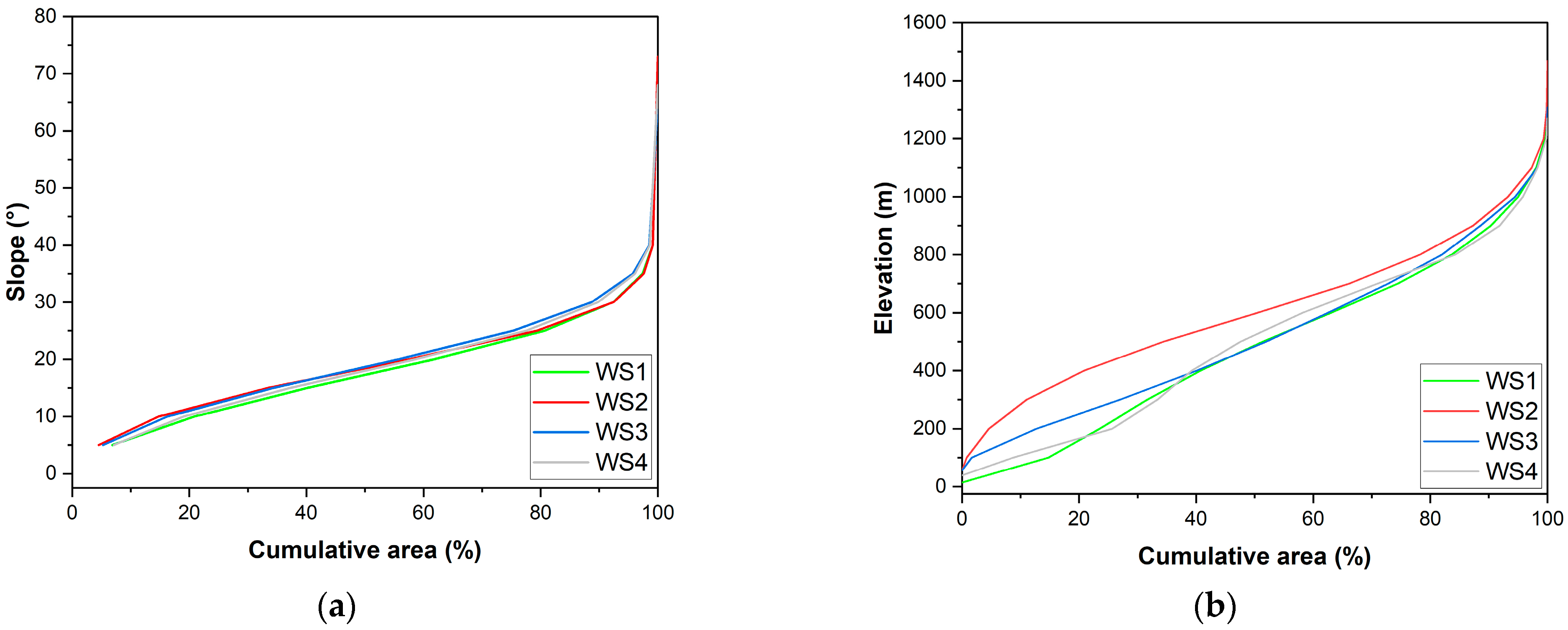
3.1.1. Hypsometric Curves

The hypsometric slope–area curves for the catchments are quite similar, with 80% of the catchment areas having slopes between 5 and 25 degrees, and 20% of the catchment areas with slopes above 25 degrees (Figure 4). The elevation–area hypsometric curves for each catchment are more diverse. WS1 and WS4 have two inflection points, one at 20–30% of the cumulative area, and another at 70–80% of the cumulative area. WS3′s curve is initially fairly linear but becomes concave at higher elevations. WS2′s curve shows a marked S-shape, which seems to indicate that WS2 is in a younger geomorphic stage compared to the other three catchments, which are approaching the mature/old stage [48].

3.1.2. Correlation between CDs

In the first step, the least correlated variables within each attribute were selected based on Figure 5a. As a result, only Slope, Kg, and Dd were retained out of the 14 topographic (T) attributes. Among the four-land cover (LC) attributes, only the CN_est was selected. Ferra, S-C, S-C-L, and OC were chosen from the 11 soil attributes. Finally, Gran and Gneiss were kept among the geology (G) attributes.
Figure 5b was used to assess the between-group correlations, i.e., correlations between CDs from different groups. Kg (T) was found to be positively correlated with CN_est (LC) and negatively correlated with Ferra (S), S-C-L (S), and Gneiss (G). Additionally, there was a strong correlation between Slope (T) and OC (S), as well as between Dd (T) and S-C (S) and between Dd and Gran (G). CN_est (LC) is correlated negatively with both Ferra (S) and Gneiss (G). Finally, S-C (S) shows a positive correlation with Gran (G), and S-C-L (S) is positively correlated with Gneiss (G).

3.2. Hydrological Signatures and Their Spatial Patterns

3.2.1. Rainfall Characteristics

Most rainfall fell between mid-December and mid-April (wet rainy season, Figure 6). The cumulative rainfall amount varied across the catchments during the study period. Specifically, WS4 in the western part received the highest amount of rainfall (~1800 mm), whereas WS3 in the eastern part received the lowest amount of rainfall (~1670 mm).

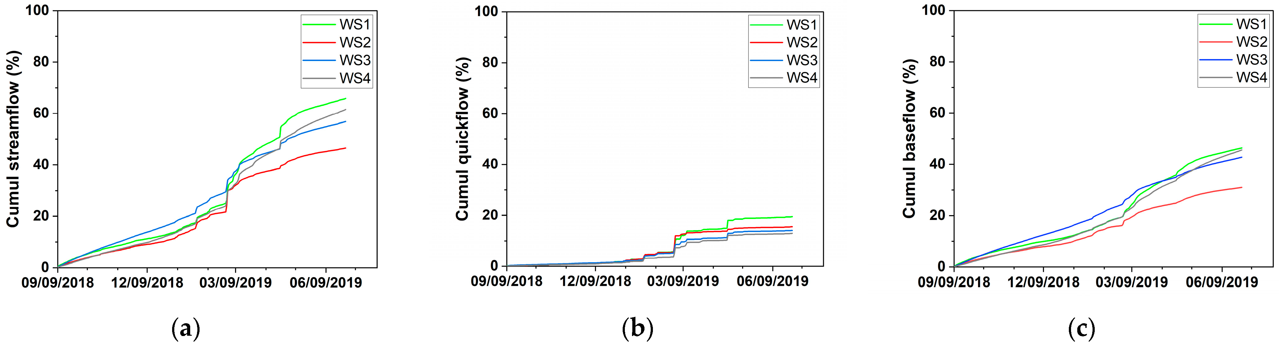
3.2.2. Streamflow Characteristics

In terms of flow distribution (Figure 7a), WS1 had the highest cumulative flow during the study period, accounting for 66% of total rainfall, while WS2 had the lowest (46%). When considering cumulative quickflow (Figure 7b), WS1 had the highest value (20% of total rainfall), whereas WS2, WS3, and WS4 had fairly similar values (12–15%). In terms of cumulative baseflow (Figure 7c), WS1, WS4, and WS3 had similar values (42–46% of total rainfall), while WS2 had noticeably lower values (31%).

3.2.3. Streamflow Characteristics

The flow duration curve (Figure 8) reveals that the ‘high flows’ (0–5% exceedance probability) for all the watersheds are relatively similar. The curves differ more strongly in the medium flow range (20–80 percent), with WS1, WS3, and WS4 displaying the highest values and WS2 having the lowest. In terms of low flows (95–100% exceedance probability), the WS2 and WS1, in that order, exhibit the lowest, while the WS3 and WS4 have the highest.

3.2.4. Hydrological Signatures

The BFI values range from 0.60 to 0.68, with the watersheds ranked in ascending order, as follows: WS2, WS1, WS3, and WS4 (Figure 9a). Values of rc, Qp, and ts are highly variable across events in all four watersheds (Figure 9b–d). Considering the mean values, we can observe that the runoff coefficient range between 0.09 and 0.34, with WS2 displaying the lowest value, followed by WS3, WS4, and WS1. Mean peak discharge Qp ranges from 0.34 to 1.38 mm/h, with WS2 having the lowest value, followed by WS1 and WS3, while WS4 shows the highest value. Regarding the runoff event time scales, they range between 0.11 and 0.22 h/km, with WS4 having the highest value, followed by WS1, WS3, and WS2 in descending order. Additionally, the low flows Q95 follow a similar trend to the BFI. Finally, the high flows Q5 and mean discharge generated by WS1 are the highest, followed by WS4 and WS3, while the lowest value pertains to WS2 (Figure 9e).

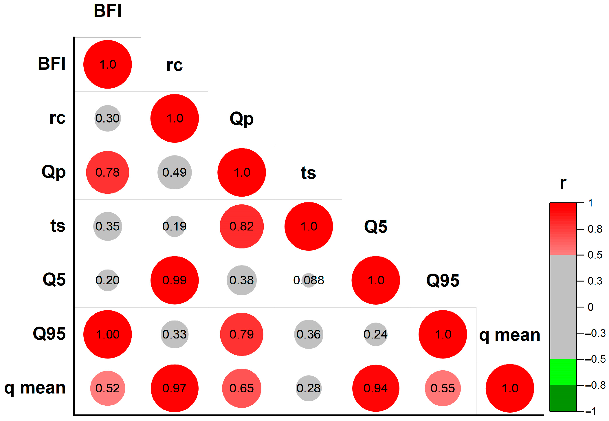
3.2.5. Correlation between Hydrological Signatures

According to Figure 10, there are strong correlations between the hydrological variables. Specifically, BFI exhibits a strong positive correlation with Q95 (low flows). rc is positively correlated with Q5 and q_mean, while Qp is related to ts. Furthermore, there is a strong correlation between Q5 and q_mean.

3.3. Correlation between Selected CDs and HSs

The correlation plot shows links between the selected catchment descriptors (CDs) and the hydrological signatures (HSs). However, not all the strong correlations (indicated by red and green circles) are reliable due to the strong dependence on a single ‘high leverage’ point. Accordingly, we added an ‘*’ to indicate a robust correlation. As a result, each HS was found to be correlated with at least two or more CDs (Figure 11).
Specifically, BFI and Q95 both exhibit a positive correlation with Kg (T) and CN_est (LC), and a negative correlation with Ferra (S), S-C-L (S), and Gneiss (G). rc is negatively correlated with Slope (T) and Ferra (S), while Qp is positively correlated with Kg (T) and negatively with Ferra (S) and Gneiss (G). ts is negatively correlated with S-C (S) and Gran (G). Q5 is negatively related to Slope (T) and OC (S), while q_mean is negatively correlated with Ferra (S).

4. Discussion

4.1. General Hydrological Characteristics

The study period (September 2018–June 2019) can be qualified as a normal year. The cumulative rainfall curves clearly show a distinct wet rainy and dry (but still rainy) season. The hot and wet rainy season occurs from December to April, while the cool and dry season occurs from May to November. During the rainy season, the region receives a large amount of precipitation, but this does not immediately translate into increased river discharge. Indeed, although rainfall increases sharply as of December, notable changes in the cumulative streamflow happen only as of February, which is likely due to a slow response time of the groundwater table. Conversely, during the dry season, the region receives little precipitation, resulting in a period of low flows in the rivers. This strong seasonality of rainfall and river discharge in the northeastern region of Madagascar is the result of a complex interplay between several atmospheric and oceanic processes, such as convective precipitation and trade winds, as well as the movement of the intertropical convergence zone (ITCZ) [62]. Specifically, the position of the ITCZ shifts northward from March to August and southward between September and December, resulting in distinct rainy and dry seasons in tropical regions [63,64].
The proportion of precipitation that turns into streamflow within the Ankavia basin is somewhat variable, ranging from 40% to 60% depending on the watershed. Generally, in humid regions with well-drained soils and gentle topography, such as parts of the eastern United States, Europe, and Southeast Asia, the proportion of rainfall that becomes streamflow is lower, ranging from about 10% to 40% [65,66]. On the other hand, in arid and semi-arid regions characterized by limited vegetation cover and poorly drained soil, the streamflow proportion ranges from approximately 20% to 60% [67]. In tropical regions with highly drained soils and rugged topography, such as those in Asia and Brazil, the proportion of precipitation that flows as streamflow ranges from 30% to 60%, and sometimes can exceed 90% during extreme events [68,69]. Finally, in mountainous areas with high precipitation and steep topography, such as the Andes, the Alps, and the Himalayas, this rate can reach up to 80% or more [70]. Therefore, the discharge-to-rainfall ratio observed in the Ankavia basin appears consistent with observations from tropical regions with highly drained soils and rugged topography.
The calculated BFI values in this study range from 0.60 to 0.68, which is consistent with studies conducted in Brazil [71] and Indonesia [72] in similar environments. However, other regions in Indonesia have shown smaller BFI values (ranging from 0.49 to 0.56) compared to Ankavia [73]. In contrast, higher BFI values were reported for watersheds in Thailand [74] and Malaysia [75].
The study findings show that the mean runoff coefficient values range from 0.09 to 0.34, which is consistent with similar research conducted on meso-scale watersheds in Brazil [71] and in West Africa [76]. However, the observed rc values are slightly higher than the value reported in other parts of Brazil [77], ranging from approximately 0.008 to 0.12, and lower than the value estimated in Malaysia [78], ranging from 0.32 to 0.92. Additionally, some runoff coefficient values greater than 1 were observed in this study, especially during some extreme events, which is theoretically impossible since the amount of rainfall should always be greater than the volume of runoff. This could be due to several factors. Firstly, the rainfall data used in the study were obtained from IMERG and are known to underestimate some classes of rainfall, in particular, extreme rainfall events (>100 mm/d) [45]. Additionally, the method used to separate the hydrographs could also contribute to uncertainty in the estimation of runoff. Moreover, since the rating curve was extrapolated for high water, the runoff during extreme events may be biased (possibly overestimated).
The mean peak discharge and runoff event time scales in the Ankavia watershed range from 0.34 to 1.38 mm/h and 0.11 to 0.22 h/km, respectively. It is important to note that a wide range of values for these two hydrological signatures are found in the literature, which means that there are more dependent on basin characteristics, rather than the specific tropical regions themselves [79,80,81].
When compared to other tropical regions, the Ankavia River in Madagascar has a slightly higher range of flow rate values. For instance, the Sapucaí River in Brazil [68], the Mae Klong River in Thailand [82], and the Mekong River in Vietnam [83] have flow rates (Q5, q_mean, Q95) of (5.48, 2.45, 1.33), (5.6, 2.19, 1.11), and (2.50, 1.74, 1.06) [mm/d], respectively. The region where the Ankavia River is located receives high levels of precipitation, which contributes to its relatively high flow rate even in normal years such as 2019 (~1800 mm). Overall, the Ankavia River exhibits similar discharge values when compared to other basins studied in the SAVA region. For instance, the Lokoho River, which is located to the north of the Ankavia basin, has (Q5, q_mean, Q95) of (7.83, 4.5, 1.94), as reported by ref. [37]. Similarly, the Sambirano River, situated further north, has a Q95 flow of 1.29 mm/d and an average flow of 4.06 mm/d [64]. Hence, the observed range of values in this study falls within the ‘normal’ range for rivers in the SAVA region, Madagascar [64].

4.2. Catchment Descriptors

We examined all the catchment attributes using the correlation matrix based on Pearson’s coefficient (Figure 5a). A critical analysis of these correlations is crucial before deriving any linkages; otherwise, potentially misleading relationships may be inferred [84]. In addition, strong correlations between two or more attributes belonging to the same group may arise because these parameters roughly evaluate the same characteristics. This is for instance the case with the attributes related to catchment area and perimeter (Kg, Cc, Re, etc.) which all determine the watershed morphometry.
The strong relationships that have been found between CDs of different groups in the present study can be explained by the spatial distribution of these CDs in the Ankavia watershed (Figure 2 and Table S1). For instance, WS2 has a more compact and rougher landscape, lower CN (i.e., higher forest cover), more Ferrasols, more SCL soils, and more Gneiss than the other WSs. In contrast, WS3 and WS4 are more elongated, less rough, have higher CN (i.e., lower forest cover), and more Acrisols and CL soils than WS2. The differences in land cover characteristics are likely due to the absence of secondary roads and navigable rivers in WS2, making it less accessible and, therefore, less prone to human activity. Moreover, the presence of natural parks and protected areas in WS2 also probably contributes to its higher forest cover.
The distribution of soils in the watershed depends on various factors such as topography, climate, and geology. In our case study, Acrisols dominate in the downstream (northeast) part, while Ferrasols dominate in the upstream (southwest) part of the watershed. Typically, Acrisols are found on erosive slopes of low hills while Ferrasols are found on adjacent stable pediments or high hills [43].

4.3. Which Catchment Descriptors Are the Best Predictors for Each Hydrological Signature?

The BFI calculated in this study ranges from 0.60 (WS2) to 0.68 (WS4) and is positively correlated with CN_est, the latter being negatively correlated with the forest cover. Land cover attributes thus appear to be an important predictor of baseflow (BFI). Indeed, forest cover has a higher evapotranspiration rate than cropland, degraded land, and tree fallow cover, which may explain why BFI declines as forests cover increases [85,86]. This is consistent with other studies conducted in Brazil [71] and Indonesia [72]. However, some studies contradict this finding, such as a study conducted in the southern Amazon [71], which reported a higher BFI in forested areas than in grazing areas, supporting the “sponge effect theory” [19] that forested watersheds produce more baseflow during the dry season than watersheds with disturbed vegetation [87].
BFI also appears to be correlated with Kg and the relative area occupied by Ferralsols (and sandy clay soils). The positive correlation with Kg is likely the result of a confounding effect since Kg is highly correlated with CN_est (the most forested watershed is also the most compact). The negative correlation with Ferralsols may also be spurious, as Ferralsols are negatively correlated with CN_est. Indeed, Ferralsols are known to have favorable physical properties, especially high infiltration capabilities [88]. A higher BFI would, therefore, be expected in Ferralsol-dominated watersheds, which is not observed here. Similarly, the negative correlation with gneiss may also be spurious, especially since fractured hard rocks such as quartzites and gneisses more generally lead to aquifers reservoirs with high capacities [56].
The mean runoff coefficient values in our study range from 0.09 to 0.34, depending on the watershed. The WS2 watershed, which has a higher proportion of Ferralsols and forest compared to the other basins (Figure 2c), has the lowest runoff coefficient. Ferralsols are known for their excellent physical properties, including high permeability due to their well-developed microaggregate structure, sometimes referred to as “pseudo-sands” [89]. Conversely, Acrisols, present mainly downstream of the basin, have a poorer structure and horizons with clay accumulation, which may explain higher runoff, particularly if the soil is cultivated. While the correlation is not strong, we observe that the runoff coefficient is lower in WS2 (Figure 9b), which has the most forested cover, and higher in the other less forested WSs. This observation is consistent with the well-known role of forest cover in intercepting rainwater (litter and canopy) and protecting and improving the hydrological conditions of the soil thanks to the litter layer that accumulates on the surface. The average slope is negatively correlated with the runoff coefficient, but this relationship is most likely spurious since the range of average slopes across the watersheds is small (~2°) and topographic parameters may not significantly affect the runoff coefficient [8]. Other studies have also demonstrated a strong correlation between runoff coefficient, soil properties, and land cover characteristics, such as those conducted by ref. [71] in Brazil and by ref. [76] in West Africa.
The mean peak discharge in the Ankavia catchment ranges from 0.34 mm/h to 1.38 mm/h. The peak discharge of WS2 is found to be the lowest compared to the other three WSs. In this case study, there appears to be a positive correlation between Qp and Kg (T); however, this relationship may be spurious. Indeed, more compact watersheds are expected to lead to shorter response times and higher peak discharges. Instead, the relationship between Qp and runoff/quickflow (rc) seems more relevant. Indeed, the positive relationship between these two parameters is well-established in the literature, indicating that if runoff increases (rc), Qp also increases [47]. Therefore, predictors of runoff coefficients, such as soil type, are also predictors for peak discharge.
The WS1, WS2, and WS3 catchments exhibit faster hydrologic responses (lower runoff event time scale ts) compared to WS4, which is located towards the west. Our correlation analysis suggests a strong positive relationship between Qp and ts (Figure 10). Meanwhile, soil attributes, which are critical factors for runoff, also appear to contribute to the hydrologic responsiveness of the catchments (Figure 11). Additionally, we observed that WS4 has the lowest proportion of granite and the highest proportion of shale.
The correlation analysis reveals that Q5 and q_mean are positively correlated with rc and that Q95 is positively correlated with BFI (Figure 10). Q5 (high flows) is the result of runoff, and factors that are good predictors of rc, such as soil attributes, are therefore also good at predicting Q5. It is worthing that the mean discharge values are heavily influenced by extreme values. Hence, soil attributes that are predictors of rc and Q5 also serve as good predictors for q_mean. Q95 (low flows) originate from soil releases, groundwater, or channel storage; hence, catchment descriptors for predicting the BFI and Q95 are expected to be roughly the same (Figure 11).
In summary, the more forested WS2 watershed has a better flood buffering capacity (lower Q5 and Qp values), but lower BFI (potentially due to higher ET). Consequently, this watershed experiences more pronounced low flows during the dry season (lower Q95 values). In contrast, the less forested WS3 and WS4 watersheds (and to a lesser extent WS1) have higher Q5 and Qp values, which indicates a lower flood buffering capacity than WS2. Nevertheless, they have higher BFI than WS2, resulting in less pronounced low flows (higher Q95) during the dry season.

5. Conclusions

In this study, we aimed at gaining a better understanding of the factors driving the hydrological response of the Ankavia watershed by investigating the linkages between watershed descriptors and hydrological signatures using a fairly unique dataset for northeastern Madagascar. Our findings indicate that all watershed attributes play a role in governing hydrological responses to a greater or lesser extent. Land cover, soil properties, and geology are the best predictors of baseflow and low flows (Q95). In contrast, soil properties mainly govern the runoff coefficient (rc), mean discharge (q_mean), peak flow (Qp), and runoff event time scales (ts).
The findings indicate that the WS2 watershed, primarily covered by forests, has the lowest runoff coefficients and peak flows. This emphasizes the importance of protecting the forest cover in this area, not just to protect biodiversity but also to mitigate downstream flooding risks. However, this watershed is also characterized by the lowest low flows (Q95), reflecting a limited capacity for maintaining sufficient discharge during the dry season. Furthermore, the notably higher peak discharges in WS3 and WS4 vs. WS2 highlight the impact of land cover on the hydrological characteristics of the river basin, which suggest that human activities, such as deforestation, shifting cultivation, as well as agriculture, can have a considerable impact on the hydrological behavior, and must be considered in water resource management in the SAVA region.
This study highlights the complexity of the interactions between the factors governing hydrological systems in a large tropical watershed. Nevertheless, the findings can serve as a basis for interpreting hydrological responses in other ungauged basins within the SAVA region but also more generally in the northeastern part of Madagascar that are under similar hydrological conditions. Ultimately, the study provides valuable insights into the hydrological characteristics of the sub-basins within the Ankavia watershed and underscores the significance of sustainable land use practices and conservation efforts for effective watershed management.

Supplementary Materials

The following supporting information can be downloaded at: https://www.mdpi.com/article/10.3390/w15122237/s1, Table S1: catchment descriptors; Table S2: hydrological signatures; Figure S1: correlation between the selected CDs and WSs.

Author Contributions

Conceptualization, Z.R. and C.L.B.; methodology, Z.R. and C.L.B.; software, Z.R.; validation, Z.R., C.L.B. and A.R.; formal analysis, Z.R. and C.L.B.; investigation, Z.R.; resources, Z.R.; data curation, Z.R.; writing—original draft preparation, Z.R.; writing—review and editing, Z.R., C.L.B., A.R. and M.V.; visualization, Z.R., C.L.B., and A.R.; supervision, C.L.B. and A.R.; project administration, Z.R., C.L.B., A.R. and M.V.; funding acquisition, M.V. All authors have read and agreed to the published version of the manuscript.

Funding

This research and APC fees are funded by the Belgian Académie de Recherche d’Enseignement Supérieur (ARES-CCD: www.ares-ac.be, accessed on 14 April 2023), through the 2017 Research Project for Development (PRD) in Madagascar, named: Renforcement des Capacités en Gestion Intégrée des Ressources en Eau (GIRE-SAVA). More information is avaialble: https://uclouvain.be/fr/chercher/louvain4water/gire-sava-renforcement-des-capacites-en-gestion-integree-des-ressources-en-eau-de-la-region-sava.html (accessed on 14 April 2023).

Data Availability Statement

The observed discharge data used in this study are from the GIRE SAVA project (available on request).

Acknowledgments

The authors acknowledge all those who gave their support for this study to be accomplished. Our special thanks go to the south coordinator Joseph Benitsiafantoka (2017–2021), Christophe Manjaribe (since 2021), and their respective staff in the Centre Universitaire Régional de la SAVA (CURSA). We also acknowledge the contribution of the members of the Sambava regional direction of water, especially Tsirinasy (2017–2021), Carlos Totomalaza (since 2021), the heads of the surveyed communities, and the survey participants (technician Sabe Christian and research assistants).

Conflicts of Interest

The authors declare no conflict of interest. The funders had no role in the design of the study; in the collection, analyses, or interpretation of data; in the writing of the manuscript; or in the decision to publish the results.

Appendix A

Figure A1. Pictures of the riverbed, banks, and the limnimetrics stations.
Water 15 02237 g0a1

Appendix B

Figure A2. Rating curves of the four sub catchments (WS1–WS4) in the Ankavia watershed.
Water 15 02237 g0a2

Appendix C

Figure A3. Hydrograph separation (Daily Time Scale).
Water 15 02237 g0a3

References

  1. Wu, Q.; Ke, L.; Wang, J.; Pavelsky, T.M.; Allen, G.H.; Sheng, Y.; Duan, X.; Zhu, Y.; Wu, J.; Wang, L. Satellites Reveal Hotspots of Global River Extent Change. Nat. Commun. 2023, 14, 1587. [Google Scholar] [CrossRef] [PubMed]
  2. Papa, F.; Crétaux, J.-F.; Grippa, M.; Robert, E.; Trigg, M.; Tshimanga, R.M.; Kitambo, B.; Paris, A.; Carr, A.; Fleischmann, A.S. Water Resources in Africa under Global Change: Monitoring Surface Waters from Space. Surv. Geophys. 2023, 44, 43–93. [Google Scholar] [CrossRef] [PubMed]
  3. Group, A.H.; Vörösmarty, C.; Askew, A.; Grabs, W.; Barry, R.G.; Birkett, C.; Döll, P.; Goodison, B.; Hall, A.; Jenne, R. Global Water Data: A Newly Endangered Species. Eos Trans. Am. Geophys. Union 2001, 82, 54–58. [Google Scholar]
  4. Godinez-Madrigal, J.; Van Cauwenbergh, N.; van der Zaag, P. Production of Competing Water Knowledge in the Face of Water Crises: Revisiting the IWRM Success Story of the Lerma-Chapala Basin, Mexico. Geoforum 2019, 103, 3–15. [Google Scholar] [CrossRef]
  5. Bezerra, M.O.; Vollmer, D.; Souter, N.J.; Shaad, K.; Hauck, S.; Marques, M.C.; Mtshali, S.; Acero, N.; Zhang, Y.; Mendoza, E. Stakeholder Engagement and Knowledge Co-Production for Better Watershed Management with the Freshwater Health Index. Curr. Res. Environ. Sustain. 2023, 5, 100206. [Google Scholar] [CrossRef]
  6. Kong, M.; Zhao, J.; Zang, C.; Li, Y.; Deng, J. Characteristics and Driving Mechanism of Water Resources Trend Change in Hanjiang River Basin. Int. J. Environ. Res. Public Health 2023, 20, 3764. [Google Scholar] [CrossRef]
  7. Blöschl, G.; Sivapalan, M. Scale Issues in Hydrological Modelling: A Review. Hydrol. Process. 1995, 9, 251–290. [Google Scholar] [CrossRef]
  8. Blöschl, G.; Sivapalan, M.; Wagener, T. Runoff Prediction in Ungauged Basins; Cambridge University Press: Cambridge, UK, 2013; p. 492. [Google Scholar]
  9. Merz, R.; Blöschl, G.; Parajka, J. Regionalization Methods in Rainfall–Runoff Modelling Using Large Catchment Samples; IAHS Publication: Oxfordshire, UK, 2006; 9p. [Google Scholar]
  10. van Soesbergen, A.; Mulligan, M. Uncertainty in Data for Hydrological Ecosystem Services Modelling: Potential Implications for Estimating Services and Beneficiaries for the CAZ Madagascar. Ecosyst. Serv. 2018, 33, 175–186. [Google Scholar] [CrossRef]
  11. Eckstein, D.; Künzel, V.; Schäfer, L. Global Climate Risk Index 2021. Who Suffers Most from Extreme Weather Events? In Weather-Related Loss Events in 2019 and 2000 to 2019; Germanwatch eV: Bonn, Germany, 2021. [Google Scholar]
  12. Qazi, N. Hydrological Functioning of Forested Catchments, Central Himalayan Region, India. For. Ecosyst. 2020, 7, 63. [Google Scholar] [CrossRef]
  13. Fritsch, J.-M. Les Effets Hydrologiques Du Déboisement de La Forêt Amazonienne et d’utilisations Alternatives Du Sol. In Colloques et Séminaires-Institut Français de Recherche Scientifique pour le Développement en Coopération; Bibliothèque Populaire du Développement: Dakar, Senegal, 1995; pp. 411–424. [Google Scholar]
  14. Wu, S.; Zhao, J.; Wang, H.; Sivapalan, M. Regional Patterns and Physical Controls of Streamflow Generation Across the Conterminous United States. Water Resour. Res. 2021, 57, e2020WR028086. [Google Scholar] [CrossRef]
  15. Choubin, B.; Solaimani, K.; Rezanezhad, F.; Habibnejad Roshan, M.; Malekian, A.; Shamshirband, S. Streamflow Regionalization Using a Similarity Approach in Ungauged Basins: Application of the Geo-Environmental Signatures in the Karkheh River Basin, Iran. CATENA 2019, 182, 104128. [Google Scholar] [CrossRef]
  16. Ochoa-Tocachi, B.F.; Buytaert, W.; De Bièvre, B. Regionalization of Land-Use Impacts on Streamflow Using a Network of Paired Catchments. Water Resour. Res. 2016, 52, 6710–6729. [Google Scholar] [CrossRef] [Green Version]
  17. Gay-des-Combes, J.M.; Robroek, B.J.M.; Hervé, D.; Guillaume, T.; Pistocchi, C.; Mills, R.T.E.; Buttler, A. Slash-and-Burn Agriculture and Tropical Cyclone Activity in Madagascar: Implication for Soil Fertility Dynamics and Corn Performance. Agric. Ecosyst. Environ. 2017, 239, 207–218. [Google Scholar] [CrossRef]
  18. Baumann, J. Tropical Watersheds, Hydrological Processes. In Encyclopedia of Agrophysics; Gliński, J., Horabik, J., Lipiec, J., Eds.; Springer: Dordrecht, The Netherlands, 2011; pp. 937–938. ISBN 978-90-481-3585-1. [Google Scholar]
  19. Bruijnzeel, L.A. Hydrological Functions of Tropical Forests: Not Seeing the Soil for the Trees? Agric. Ecosyst. Environ. 2004, 104, 185–228. [Google Scholar] [CrossRef]
  20. Hou, Y.; Zhang, M.; Meng, Z.; Liu, S.; Sun, P.; Yang, T. Assessing the Impact of Forest Change and Climate Variability on Dry Season Runoff by an Improved Single Watershed Approach: A Comparative Study in Two Large Watersheds, China. Forests 2018, 9, 46. [Google Scholar] [CrossRef] [Green Version]
  21. D’Almeida, C.; Vörösmarty, C.J.; Hurtt, G.C.; Marengo, J.A.; Dingman, S.L.; Keim, B.D. The Effects of Deforestation on the Hydrological Cycle in Amazonia: A Review on Scale and Resolution. Int. J. Climatol. A J. R. Meteorol. Soc. 2007, 27, 633–647. [Google Scholar] [CrossRef]
  22. Cui, X.; Graf, H.-F.; Langmann, B.; Chen, W.; Huang, R. Hydrological Impacts of Deforestation on the Southeast Tibetan Plateau. Earth Interact. 2007, 11, 1–18. [Google Scholar] [CrossRef]
  23. Arias, M.E.; Lee, E.; Farinosi, F.; Pereira, F.F.; Moorcroft, P.R. Decoupling the Effects of Deforestation and Climate Variability in the T Apajós River Basin in the B Razilian A Mazon. Hydrol. Process. 2018, 32, 1648–1663. [Google Scholar] [CrossRef]
  24. Thanapakpawin, P.; Richey, J.; Thomas, D.; Rodda, S.; Campbell, B.; Logsdon, M. Effects of Landuse Change on the Hydrologic Regime of the Mae Chaem River Basin, NW Thailand. J. Hydrol. 2007, 334, 215–230. [Google Scholar] [CrossRef]
  25. Wilk, J.; Andersson, L.; Plermkamon, V. Hydrological Impacts of Forest Conversion to Agriculture in a Large River Basin in Northeast Thailand. Hydrol. Process. 2001, 15, 2729–2748. [Google Scholar] [CrossRef]
  26. Sivapalan, M.; Takeuchi, K.; Franks, S.W.; Gupta, V.K.; Karambiri, H.; Lakshmi, V.; Liang, X.; Mcdonnell, J.J.; Mendiondo, E.M.; O’Connell, P.E.; et al. IAHS Decade on Predictions in Ungauged Basins (PUB), 2003–2012: Shaping an Exciting Future for the Hydrological Sciences. Hydrol. Sci. J. 2003, 48, 857–880. [Google Scholar] [CrossRef] [Green Version]
  27. WMO. Climate Change Increased Extreme Rainfall in Southeast Africa Storms—Madagascar. Available online: https://reliefweb.int/report/madagascar/climate-change-increased-extreme-rainfall-southeast-africa-storms (accessed on 2 October 2022).
  28. Rabefitia, Z. Le Changement Climatique à Madagascar; Direction Générale de la Météorologie: Antananarivo, Madagascar, 2008; 32p. [Google Scholar]
  29. AFD. Madagascar—Rural Drinking Water Supply and Sanitation Programme—Appraisal Report; African Development Fund: Tunis, Tunisia, 2005; p. 75. [Google Scholar]
  30. Ralaingita, M.; Ennis, G.; Russell-Smith, J.; Sangha, K.; Razanakoto, T. The Kere of Madagascar: A Qualitative Exploration of Community Experiences and Perspectives. Ecol. Soc. 2022, 27, 42. [Google Scholar] [CrossRef]
  31. Tadross, M.; Randriamarolaza, L.; Rabefitia, Z.; Zheng, K.Y. Climate Change in Madagascar; Recent Past and Future; World Bank: Washington, DC, USA, 2008; p. 18. [Google Scholar]
  32. Aubert, S.; Razafiarison, S.; Bertrand, A. Déforestation et Systèmes Agraires à Madagascar: Les Dynamiques Des Tavy Sur La Côte Orientale; Editions Quae: Versailles, France, 2003. [Google Scholar]
  33. Pereira, D.d.R.; Almeida, A.Q.d.; Martinez, M.A.; Rosa, D.R.Q. Impacts of Deforestation on Water Balance Components of a Watershed on the Brazilian East Coast. Rev. Bras. De Ciência Do Solo 2014, 38, 1350–1358. [Google Scholar] [CrossRef] [Green Version]
  34. Gade, D.W. Deforestation and Its Effects in Highland Madagascar. Mt. Res. Dev. 1996, 16, 101–116. [Google Scholar] [CrossRef]
  35. CPGU. Atlas de La Vulnérabilité Sectorielle de La Région SAVA; Cellule de Prevention et de la Gestion des Urgences: Antananarivo, Madagascar, 2012. [Google Scholar]
  36. INSTAT. Résultats Globaux Du Recensement Général de La Population et de l’habitation de 2018 de Madagascar. Available online: https://madagascar.unfpa.org/sites/default/files/pub-pdf/resultat_globaux_rgph3_tome_01.pdf (accessed on 21 November 2022).
  37. Randriamaherisoa, A.; Binard, M. Régionalisation Des Paramètres Du Modèle Maillé: Impact de La Déforestation Sur Le Régime Hydrologique de La Lokoho (Madagascar). In Acte des VIII Journées Hydrologiques de l’ORSTOM: Régionalisation en Hydrologie-Application au Développement; ORSTOM: Montpellier, France, 1992; pp. 223–232. [Google Scholar]
  38. CREAM. Monographie de La Région SAVA. 2013. Available online: https://www.pseau.org/outils/ouvrages/mg_mef_monographie-region-sava_2014.pdf (accessed on 23 July 2022).
  39. Bauer, W.; Walsh, G.J.; De Waele, B.; Thomas, R.J.; Horstwood, M.S.; Bracciali, L.; Schofield, D.I.; Wollenberg, U.; Lidke, D.J.; Rasaona, I.T. Cover Sequences at the Northern Margin of the Antongil Craton, NE Madagascar. Precambrian Res. 2011, 189, 292–312. [Google Scholar] [CrossRef]
  40. Palm, C.A.; Swift, M.J.; Woomer, P.L. Soil Biological Dynamics in Slash-and-Burn Agriculture. Agric. Ecosyst. Environ. 1996, 58, 61–74. [Google Scholar] [CrossRef]
  41. Earth Resources Observation and Science (EROS) Center Shuttle Radar Topography Mission (SRTM) 1 Arc-Second Global. 2017. Available online: https://www.usgs.gov/centers/eros/science/usgs-eros-archive-digital-elevation-shuttle-radar-topography-mission-srtm-1 (accessed on 3 June 2022).
  42. Bontemps, S.; Defourny, P.; Van Bogaert, E.; Team, E.S.A.; Arino, O.; Kalogirou, V.; Perez, J.R. GLOBCOVER 2009 Products Description and Validation Report; European Space Agency: Paris, France, 2009. [Google Scholar]
  43. Hengl, T.; Mendes de Jesus, J.; Heuvelink, G.B.M.; Ruiperez Gonzalez, M.; Kilibarda, M.; Blagotić, A.; Shangguan, W.; Wright, M.N.; Geng, X.; Bauer-Marschallinger, B.; et al. SoilGrids250m: Global Gridded Soil Information Based on Machine Learning. PLoS ONE 2017, 12, e0169748. [Google Scholar] [CrossRef] [Green Version]
  44. Ross, C.W.; Prihodko, L.; Anchang, J.; Kumar, S.; Ji, W.; Hanan, N.P. HYSOGs250m, Global Gridded Hydrologic Soil Groups for Curve-Number-Based Runoff Modeling. Sci. Data 2018, 5, 180091. [Google Scholar] [CrossRef]
  45. Ramahaimandimby, Z.; Randriamaherisoa, A.; Jonard, F.; Vanclooster, M.; Bielders, C.L. Reliability of Gridded Precipitation Products for Water Management Studies: The Case of the Ankavia River Basin in Madagascar. Remote Sens. 2022, 14, 3940. [Google Scholar] [CrossRef]
  46. Huffman, G.J.; Bolvin, D.T.; Braithwaite, D.; Hsu, K.-L.; Joyce, R.J.; Kidd, C.; Nelkin, E.J.; Sorooshian, S.; Stocker, E.F.; Tan, J. Integrated Multi-Satellite Retrievals for the Global Precipitation Measurement (GPM) Mission (IMERG). In Satellite Precipitation Measurement; Springer: Berlin/Heidelberg, Germany, 2020; pp. 343–353. [Google Scholar]
  47. Horton, R.E. Drainage-Basin Characteristics. Trans. AGU 1932, 13, 350. [Google Scholar] [CrossRef]
  48. Strahler, A.N. Hypsometric (Area-Altitude) Analysis of Erosional Topography. GSA Bull. 1952, 63, 1117–1142. [Google Scholar] [CrossRef]
  49. Schumm, S.A. Evolution of Drainage Systems and Slopes in Badlands at Perth Amboy, New Jersey. Geol Soc Am. Bull 1956, 67, 597. [Google Scholar] [CrossRef]
  50. Strahler, A.N. Quantitative Analysis of Watershed Geomorphology. Eos Trans. Am. Geophys. Union 1957, 38, 913–920. [Google Scholar] [CrossRef] [Green Version]
  51. Mishra, S.K.; Singh, V.P. Soil Conservation Service Curve Number (SCS-CN) Methodology; Springer Science & Business Media: Berlin/Heidelberg, Germany, 2013; Volume 42, ISBN 94-017-0147-4. [Google Scholar]
  52. Zhang, Y.; Liu, H. Generation Mechanisms of the Water Surface Elevation Induced by a Moving Atmospheric Pressure Disturbance. Ocean Eng. 2022, 255, 111469. [Google Scholar] [CrossRef]
  53. Addor, N.; Nearing, G.; Prieto, C.; Newman, A.J.; Le Vine, N.; Clark, M.P. A Ranking of Hydrological Signatures Based on Their Predictability in Space. Water Resour. Res. 2018, 54, 8792–8812. [Google Scholar] [CrossRef] [Green Version]
  54. Eckhardt, K. How to Construct Recursive Digital Filters for Baseflow Separation. Hydrol. Process. Int. J. 2005, 19, 507–515. [Google Scholar] [CrossRef]
  55. Lim, K.J.; Engel, B.A.; Tang, Z.; Choi, J.; Kim, K.-S.; Muthukrishnan, S.; Tripathy, D. Automated Web GIS Based Hydrograph Analysis Tool, WHAT 1. JAWRA J. Am. Water Resour. Assoc. 2005, 41, 1407–1416. [Google Scholar] [CrossRef]
  56. Eckhardt, K. A Comparison of Baseflow Indices, Which Were Calculated with Seven Different Baseflow Separation Methods. J. Hydrol. 2008, 352, 168–173. [Google Scholar] [CrossRef]
  57. Eckhardt, K. Technical Note: Analytical Sensitivity Analysis of a Two Parameter Recursive Digital Baseflow Separation Filter. Hydrol. Earth Syst. Sci. 2012, 16, 451–455. [Google Scholar] [CrossRef] [Green Version]
  58. McMillan, H.; Westerberg, I.; Branger, F. Five Guidelines for Selecting Hydrological Signatures. Hydrol. Process. 2017, 31, 4757–4761. [Google Scholar] [CrossRef] [Green Version]
  59. Castellarin, A.; Botter, G.; Hughes, D.A.; Liu, S.; Ouarda, T.; Parajka, J.; Post, D.A.; Sivapalan, M.; Spence, C.; Viglione, A. Prediction of Flow Duration Curves in Ungauged Basins. In Runoff Prediction in Ungauged Basins: Synthesis across Processes, Places and Scales; Cambridge University Press: Cambridge, UK, 2013; pp. 135–162. [Google Scholar]
  60. Sawicz, K.; Wagener, T.; Sivapalan, M.; Troch, P.A.; Carrillo, G. Catchment Classification: Empirical Analysis of Hydrologic Similarity Based on Catchment Function in the Eastern USA. Hydrol. Earth Syst. Sci. Discuss. 2011, 15, 2895–2911. [Google Scholar] [CrossRef] [Green Version]
  61. Hu, S.; Shrestha, P. Examine the Impact of Land Use and Land Cover Changes on Peak Discharges of a Watershed in the Midwestern United States Using the HEC-HMS Model. Pap. Appl. Geogr. 2020, 6, 101–118. [Google Scholar] [CrossRef]
  62. Macron, C.; Richard, Y.; Garot, T.; Bessafi, M.; Pohl, B.; Ratiarison, A.; Razafindrabe, A. Intraseasonal Rainfall Variability over Madagascar. Mon. Weather Rev. 2016, 144, 1877–1885. [Google Scholar] [CrossRef]
  63. Nassor, A.; Jury, M.R. Intra-Seasonal Climate Variability of Madagascar. Part 1: Mean Summer Conditions. Meteorol. Atmos. Phys. 1998, 65, 31–41. [Google Scholar] [CrossRef]
  64. Chaperon, P.; Danloux, J.; Ferry, L. Fleuves et Rivières de Madagascar. In Monographies Hydrologiques ORSTOM; ORSTOM: Paris, France, 1993; pp. 14–854. [Google Scholar]
  65. Ghimire, U.; Agarwal, A.; Shrestha, N.K.; Daggupati, P.; Srinivasan, G.; Than, H.H. Applicability of Lumped Hydrological Models in a Data-Constrained River Basin of Asia. J. Hydrol. Eng. 2020, 25, 05020018. [Google Scholar] [CrossRef]
  66. Lee, S.; Kim, S.U. Quantification of Hydrological Responses Due to Climate Change and Human Activities over Various Time Scales in South Korea. Water 2017, 9, 34. [Google Scholar] [CrossRef] [Green Version]
  67. Kazemzadeh, M.; Malekian, A. Homogeneity Analysis of Streamflow Records in Arid and Semi-Arid Regions of Northwestern Iran. J. Arid Land 2018, 10, 493–506. [Google Scholar] [CrossRef] [Green Version]
  68. Abreu, M.C.; Fraga, M.d.S.; Almeida, L.T.d.; Silva, F.B.; Cecílio, R.A.; Lyra, G.B.; Delgado, R.C. Streamflow in the Sapucaí River Watershed, Brazil: Probabilistic Modeling, Reference Streamflow, and Regionalization. Phys. Chem. Earth Parts A/B/C 2022, 126, 103133. [Google Scholar] [CrossRef]
  69. Jayapadma, J.; Wickramaarachchi, T.N.; Silva, G.; Ishidaira, H.; Magome, J.; Souma, K. Impact of Land Use Change on Flood Peak Discharges and Runoff Volumes at the Catchment Scale. In Proceedings of the 18th Annual Meeting of the Asia Oceania Geosciences Society (AOGS 2021), Singapore, 1–6 August 2021; World Scientific: Singapore, 2022; pp. 79–81. [Google Scholar]
  70. Cassalho, F.; Beskow, S.; Vargas, M.M.; Moura, M.M.d.; Ávila, L.F.; Mello, C.R.d. Hydrological Regionalization of Maximum Stream Flows Using an Approach Based on L-Moments. RBRH 2017, 22, e27. [Google Scholar] [CrossRef]
  71. Guzha, A.C.; Nobrega, R.L.B.; Kovacs, K.; Rebola-Lichtenberg, J.; Amorim, R.S.S.; Gerold, G. Characterizing Rainfall-Runoff Signatures from Micro-Catchments with Contrasting Land Cover Characteristics in Southern Amazonia. Hydrol. Process. 2015, 29, 508–521. [Google Scholar] [CrossRef] [Green Version]
  72. Tarigan, S.; Wiegand, K.; Sunarti; Slamet, B. Minimum Forest Cover Required for Sustainable Water Flow Regulation of a Watershed: A Case Study in Jambi Province, Indonesia. Hydrol. Earth Syst. Sci. 2018, 22, 581–594. [Google Scholar] [CrossRef] [Green Version]
  73. Taufik, M. Baseflow Index Analysis for Bengawan Solo River, Indonesia. Agromet 2022, 36, 70–78. [Google Scholar] [CrossRef]
  74. Ditthakit, P.; Nakrod, S.; Viriyanantavong, N.; Tolche, A.D.; Pham, Q.B. Estimating Baseflow and Baseflow Index in Ungauged Basins Using Spatial Interpolation Techniques: A Case Study of the Southern River Basin of Thailand. Water 2021, 13, 3113. [Google Scholar] [CrossRef]
  75. Khomsiati, N.L.; Suryoputro, N.; Yulistyorini, A.; Idfi, G.; Alias, N.E.B. The Effect of Forest Area Change in Tropical Islands towards Baseflow and Streamflow. IOP Conf. Ser. Earth Environ. Sci. 2021, 847, 012032. [Google Scholar] [CrossRef]
  76. Giertz, S.; Junge, B.; Diekkrüger, B. Assessing the Effects of Land Use Change on Soil Physical Properties and Hydrological Processes in the Sub-Humid Tropical Environment of West Africa. Phys. Chem. Earth Parts A/B/C 2005, 30, 485–496. [Google Scholar] [CrossRef]
  77. Machado, R.E.; Cardoso, T.O.; Mortene, M.H. Determination of Runoff Coefficient (C) in Catchments Based on Analysis of Precipitation and Flow Events. Int. Soil Water Conserv. Res. 2022, 10, 208–216. [Google Scholar] [CrossRef]
  78. Katimon, A.; Wahab, A.K.A. Hydrologic Characteristics of a Drained Tropical Peat Catchment: Runoff Coefficients, Water Table and Flow Duration Curves. J. Teknol. 2003, 38, 39–54. [Google Scholar] [CrossRef] [Green Version]
  79. Abdulkareem, J.H.; Pradhan, B.; Sulaiman, W.N.A.; Jamil, N.R. Development of Lag Time and Time of Concentration for a Tropical Complex Catchment under the Influence of Long-Term Land Use/Land Cover (LULC) Changes. Arab. J. Geosci. 2019, 12, 101. [Google Scholar] [CrossRef]
  80. Abdulkareem, J.H.; Sulaiman, W.N.A.; Pradhan, B.; Jamil, N.R. Relationship between Design Floods and Land Use Land Cover (LULC) Changes in a Tropical Complex Catchment. Arab. J. Geosci. 2018, 11, 376. [Google Scholar] [CrossRef]
  81. Shamsuddin, S.A.; Yusop, Z.; Noguchi, S. Influence of Plantation Establishment on Discharge Characteristics in a Small Catchment of Tropical Forest. Int. J. For. Res. 2014, 2014, e408409. [Google Scholar] [CrossRef] [Green Version]
  82. Guo, H.; Bao, A.; Liu, T.; Ndayisaba, F.; He, D.; Kurban, A.; De Maeyer, P. Meteorological Drought Analysis in the Lower Mekong Basin Using Satellite-Based Long-Term CHIRPS Product. Sustainability 2017, 9, 901. [Google Scholar] [CrossRef] [Green Version]
  83. Adamson, P.T.; Rutherfurd, I.D.; Peel, M.C.; Conlan, I.A. The Hydrology of the Mekong River. In The Mekong; Elsevier: Amsterdam, The Netherlands, 2009; pp. 53–76. [Google Scholar]
  84. Tarasova, L.; Basso, S.; Zink, M.; Merz, R. Exploring Controls on Rainfall-Runoff Events: 1. Time Series-Based Event Separation and Temporal Dynamics of Event Runoff Response in Germany. Water Resour. Res. 2018, 54, 7711–7732. [Google Scholar] [CrossRef]
  85. van Meerveld, H.J.; Jones, J.P.; Ghimire, C.P.; Zwartendijk, B.W.; Lahitiana, J.; Ravelona, M.; Mulligan, M. Forest Regeneration Can Positively Contribute to Local Hydrological Ecosystem Services: Implications for Forest Landscape Restoration. J. Appl. Ecol. 2021, 58, 755–765. [Google Scholar] [CrossRef]
  86. Rodriguez-Martínez, J.; Santiago, M. The Effects of Forest Cover on Base Flow of Streams in the Mountainous Interior of Puerto Rico, 2010; U.S. Geological Survey: Reston, VA, USA, 2017. [Google Scholar]
  87. Ogden, F.L.; Crouch, T.D.; Stallard, R.F.; Hall, J.S. Effect of Land Cover and Use on Dry Season River Runoff, Runoff Efficiency, and Peak Storm Runoff in the Seasonal Tropics of Central Panama. Water Resour. Res. 2013, 49, 8443–8462. [Google Scholar] [CrossRef] [Green Version]
  88. Ramaroson, V.H.; Becquer, T.; Sá, S.O.; Razafimahatratra, H.; Delarivière, J.L.; Blavet, D.; Vendrame, P.R.S.; Rabeharisoa, L.; Rakotondrazafy, A.F.M. Mineralogical Analysis of Ferralitic Soils in Madagascar Using NIR Spectroscopy. CATENA 2018, 168, 102–109. [Google Scholar] [CrossRef]
  89. Martinez, P.; Souza, I.F. Genesis of Pseudo-Sand Structure in Oxisols from Brazil—A Review. Geoderma Reg. 2020, 22, e00292. [Google Scholar] [CrossRef]
Figure 1. Location of the Ankavia catchment (WS1) and its sub-catchments (WS2, WS3, and WS4). The map includes the location of the weather station, rain gauges, and stream gauges, as well as the grids of IMERG (a gridded rainfall dataset).
Water 15 02237 g001
Figure 2. (a) 2019 land cover of Ankavia catchment, (b) soil texture, (c) dominant soil orders, (d) hydrological soil group, (e) modified geological map. Data sources are listed in Table 1.
Water 15 02237 g002
Figure 3. Event identification and hydrograph separation.
Water 15 02237 g003
Figure 4. Hypsometric curves: (a) slope–area (b) elevation–area.
Water 15 02237 g004
Figure 5. Correlation plot between (a) all catchment descriptors, and (b) selected catchment descriptors, based on Pearson’s coefficient r. The catchment descriptors are color-coded according to their generic group: topographic (T), land cover (LC), soil (S), and geology (G). The size of the circles indicates the strength of the correlation, with red corresponding to positive and green to negative correlations. Gray circles mean poor correlation (r < |0.5|).
Water 15 02237 g005
Figure 6. Cumulative rainfall (IMERG) over the 10-month study period (September 2018–June 2019). Date on X-axis in MM/DD/YYYY format.
Water 15 02237 g006
Figure 7. Streamflow characteristics of sub-catchments (%): (a) cumulative streamflow, (b) cumulative runoff (quickflow), (c) cumulative baseflow from September 2018 to June 2019. All values are expressed relative to the total rainfall of each sub-catchment (Figure 6). Date in X-axis in MM/DD/YYYY format.
Water 15 02237 g007
Figure 8. Flow duration curve (FDC) of the four sub-catchment rivers. Note logarithmic (Log10) scale for Y axis.
Water 15 02237 g008
Figure 9. Boxplots of hydrological signatures of the Ankavia catchment sub-watersheds over the 10-month study period. (a) Baseflow index (-), (b) runoff coefficient (-), (c) peak discharge (mm/h), (d) runoff event time scale (h/km), (e) high flows Q5, mean discharge and low flows Q95 (mm/day). Box lower and upper edges correspond to the 25th (Q1) and 75th (Q3) percentiles. Whiskers extend to Q1 − 1.5IQR (lower bound) and Q3 + 1.5IQR (upper bound), with IQR = Q3 − Q1 (inter-quartile range). Points outside the box are outliers.
Water 15 02237 g009
Figure 10. Correlation plot between hydrological signatures using Pearson’s coefficient r. The size of the circles indicates the strength of the correlation, with red corresponding to positive and green to negative correlations. Gray circles mean poor correlation (r < |0.5|).
Water 15 02237 g010
Figure 11. Correlation plot between HSs and CDs using Pearson’s coefficient r. The catchment descriptors are color-coded according to their generic group: topography (T), land cover (LC), soil (S), and geology (G). The size of the circles indicates the strength of the correlation, with red corresponding to positive and green to negative correlations. Gray circles mean poor correlation (r < |0.5|). ‘*’ indicates a robust correlation.
Water 15 02237 g011
Table 1. Summary of the gridded products and maps used to characterize the Ankavia catchment.
AttributesDataSpatial Resolution/Map ScaleSources
(Accessed on January 2022)
References
TopographyDEM
(Digital Elevation Model)
30 mhttps://earthexplorer.usgs.gov/[41]
Land CoverGlobCover v2300 mhttps://maps.elie.ucl.ac.be/CCI/viewer/[42]
Soil TextureSoilGRIDs250 mhttps://soilgrids.org/[43]
Dominant Soil OrdersSoil World Reference Base (WRB)250 mhttps://soilgrids.org/[43]
Hydrological Soil GroupHYSOGs250 mhttps://daac.ornl.gov/SOILS/guides/Global_Hydrologic_Soil_Group.html[44]
GeologyPRGM1/100,000https://www.brgm.fr/fr/reference-projet-acheve/synthese-geologique-miniere-madagascar
Table 2. Description and calculation of catchment descriptors.
GroupsVariablesLabel (Units)Calculation/DescriptionReference
Topography-morphometry (T)Drainage areaA (km2)GIS calculation 1: area calculation[47]
PerimeterP (km)GIS calculation: perimeter calculation[47]
Basin lengthLb (km)GIS calculation: spatial analyst tool/hydrology
Mean slopeSl (°)GIS calculation: spatial analyst tool/surface
Elevation rangeHmin, Hmax (m)Hmin is the minimum elevation; Hmax is the maximum elevation.
Hypsometric curve The shape of a hypsometric curve is an indicator of dominant geomorphic processes at work in a watershed area. A convex curve indicates that a greater part of the watershed’s area is held relatively high in the watershed. A concave curve indicates that the bulk of the watershed’s area resides at a relatively low elevation.[48]
Gravelius coefficientKg (-)Kg = P/(2(πA)1/2)
1 < Kg < 1.5: circular shape
1.5 < Kg < 1.9: elongated shape
Effective basin widthRb (km)Rb = A/Lb
where A is the watershed area and Lb is the watershed length
Elongation ratio ReRe= 2(A/π)0.5/Lb
Re is the ratio of the diameter of a circle having the same area as the watershed to the maximum watershed length.
Re < 0.7: more elongated
0.8 < Re <0.9: oval
Re > 0.9: circular
[49]
Unit shape factor RuRu = Lb/A½
Ru is the ratio of the length of the watershed to the square root of the area.
Total reliefRr (km)Rr = Hmax − Hmin
Rr is the maximum vertical distance between the lowest (outlet) and the highest (divide) points on the valley floor of a watershed.
Relief ratioRhRh = Rr/Lb
where Rr is the total relief and Lb is the watershed length
Rh indicates the overall steepness of the drainage watershed and the intensity of erosional processes operating on the slope of the watershed.
[49]
Total stream lengthLt (km)GIS calculation: spatial analyst tool/hydrology[50]
Length of main streamLc (km)GIS calculation: spatial analyst tool/hydrology[50]
Total number of stream segmentsNuGIS calculation: spatial analyst tool/hydrology
Drainage densityDd (km/km2)Dd = Lt/A
Dd is the stream length per unit area in the watershed.
Dd < 2: very coarse density
2 < Dd < 4: coarse density
4 < Dd < 6: moderate density
6 < Dd < 8: fine density
Dd > 8: very fine density
[47]
Constant of channel maintenance Cm (km2/km)Cm = 1/Dd
Cm expresses the watershed surface required to encompass a 1 km long stretch of stream.
[49]
Ruggedness numberRnRn = Rr × Dd
Rn indicates the structural complexity of the terrain in association with relief and drainage density.
[50]
Land cover variables (LC)Land cover % of catchment area covered by the following land cover types: mosaic crop (cropland, herbaceous cover) and mosaic natural vegetation (Crop)/mosaic tree and shrub (Mos)/tree cover (Tree).
Estimated Curve Number (CN)CN_estCN_est = Σ (%land_cover(i) × CN(i))/100)
where CNi is the respective CN to land cover, which is based on USDA Curve Number. CN_Crop = 77, CN_Mos = 60, CN_Tree = 55.
[51]
Soil variables (S)Soil texture % of catchment area covered by soils having the following soil textures: sandy clay (S-C), clay loam (C-L), sandy clay loam (S-C-L).
Soil types % of catchment area covered by the following soil types:
Acrisols (Acri), Ferrasols (Ferra), Lixisols (Lixi), Cambisols (Cambi).
Soil hydrological group % of catchment area covered by the following hydrological soil group: HSG-C (H-C), HSG-D (H-D).
Organic Carbon densityOC (g/kg)OC = OC0–5cm × 1/6 + OC5–15cm × 2/6 + OC15–30cm × 1/2
Grain diameterDg (µm)Dg = %Sand × øsa + %Clay × øsi + %Silt × øc
where øsa, øsi, øc are the median particle diameter of sand, silt, clay, which are 900 µm, 25 µm, 1 µm, respectively.
Geological variables (G)Geological characteristics % of catchment area covered by the following geological classes: Gneiss (gneiss), Granites (gran.), Shales (shales), Quartzites (quartz.).
Notes: 1 Geographic Information Tool (GIS) calculations are performed using the ArcToolbox module within the ArcGIS software 10.4 version ®.
Disclaimer/Publisher’s Note: The statements, opinions and data contained in all publications are solely those of the individual author(s) and contributor(s) and not of MDPI and/or the editor(s). MDPI and/or the editor(s) disclaim responsibility for any injury to people or property resulting from any ideas, methods, instructions or products referred to in the content.

