Abstract
In recent decades, land use patterns have changed significantly in highly urbanized areas, which is usually linked with the spatial variation of surface water quality at the catchment scale, but little attention has been paid to how hydrological seasons affect this relationship. Taking Pudong New Area of Shanghai, China, as an example, this paper evaluated the influence of hydrological seasons on the relationship between land use and water quality under different hydrological buffers. It was shown that the contribution of land use to the spatial variation of water quality is approximately 30%. In addition, the explanatory ability was greatest in the average season while it was smaller in the dry and wet seasons. Land uses showed scale effects; at a smaller scale, urban areas, agricultural land and water areas were the most important land uses affected by water quality. As the buffers changed from 500 to 1500 m, the impact of urban areas decreased significantly, while that of agricultural land and water areas increased rapidly; however, when the buffer was greater than 1000 m, the explanatory ability of water areas did not increase further but remained stable. Green space is only significant at the 200 m and 500 m scales, which showed the effect of improving river quality. This study is expected to provide references for future decision making of urban construction, environmental planning and management.
1. Introduction
Different types of land use affect the spatial variation of water quality. Through land protection and land use decision making, surface water quality can be effectively improved [1,2,3,4,5] therefore, the impact of land use on water quality has become a research hotspot in recent years. In the literature, it is generally believed that research on the evolution of water quality is of great practical significance for explaining the environmental impact caused by land uses in the process of rapid urbanization, as well as land use pattern regulation and river governance [6,7,8,9,10].
Multivariate statistical analysis is the primary method to quantify the contribution of land use variables to water quality [11,12,13]. In previous studies, researchers often conducted a correlation analysis on the impact of land use on water quality at larger spatial scales. For example, agricultural land [14,15] and urban areas have a stronger impact on water quality than forestry [16]. There was a significant negative correlation between the concentration of suspended sediment and nutrient elements and the proportion of grassland area [17]. Total nitrogen and total phosphorus were strongly correlated with agricultural land, animal husbandry and urban areas [18,19]. In some regions of Africa, agricultural land is the dominant factor for river pollution, and higher vegetation coverage helps improve water quality [20]. The effect of forest change on water quality in Brazil was studied, and the results show that forest area restoration can improve water quality [21].
Many studies analyzed the effects of land use on water quality at different spatial scales [22]. In the study of Poyang Lake, it was shown that reducing the building and cultivated land within 1 km from the river and lake was necessary for water resource protection [23]. In Taihu Lake Basin, the percentage of urban land area with a buffer size between 500 and 100 m is significantly correlated with various pollutants [24].
The land use pattern had different effects on water quality in hydrological seasons. Relevant studies showed that the influence of land use on river quality is closely related to seasonal variation [25,26]. Most studies used the water quality data of a certain year or a certain time for analysis; however, due to the different precipitation conditions in hydrological seasons, there exists obvious differences in rainfall runoff pollution. Therefore, it is worth exploring whether there are differences in its impact on surface water quality, which is of great significance for the management of rainfall runoff pollution and the improvement of urban surface water quality [27].
It can be seen that further discussion on the relationship between land use and water quality at multi-scale and different hydrological periods is still necessary. In this field, there is little focus on urban areas that are greatly affected by human activities. Therefore, in order to explore the complicated effects of land use on water quality, it is necessary to understand the effects in different hydrological seasons and at various spatial scales [28,29,30,31,32].
Taking Pudong New Area of Shanghai, China, as an example, this paper detected the relationship between land use and water quality, and how different hydrological units and hydrological seasons affect this relationship. It is expected the results can provide a decision-making reference for future urban construction, environmental planning and management in cities of the developing countries.
2. Data and Methods
2.1. Study Area
Shanghai Pudong New Area is located in the east of Shanghai, bordered by the East China Sea in the east and Hangzhou Bay in the south. The resident population is 5.7820 million. Pudong New Area covers an area of 1210.5 km2, 11% of which is water areas. The territory is flat, higher in the southeast and lower in the northwest, with a ground elevation of 3.5~4.5 m, an average elevation of 3.87 m, and a coastline of 65 km. Pudong New Area is located in the coastal zone, where the East Asian monsoon prevails on the southern edge of the northern subtropical zone. It has a marine climate with four distinct seasons, abundant precipitation, and moderate temperature. Pudong New Area has experienced a series of reform and opening up, as well as urbanization construction, and has become a prosperous and developing modern city. It will become a leading area for China’s modernization.
2.2. Data and Indicators
2.2.1. Land Use
The land use data of Pudong New Area in Shanghai are from the QuickBird satellite remote sensing data in 2010, which comes from the Key Laboratory of Geographic Information Science of the Ministry of Education of East China Normal University. The scale is 1:10,000 and the spatial resolution is 1.4 m. Interpretation is required because the river width in Pudong New Area is usually greater than 3 m.
On the basis of the remote sensing image data, geometric correction, spectrum processing, image stitching, coordinate positioning, water body enhancement, etc., were performed, and regional land use data were obtained by interpreting in the ArcGIS 10.1. However, the classification systems of the existing remote sensing interpretated data are mostly based on the basic functions of land use, but seldom consider the relationship between various land use patterns and environmental responses, and there are differences in the types and degrees of pollutants produced by various land uses [33], we reclassified the land uses in Pudong New Area in 2010 (Figure 1).
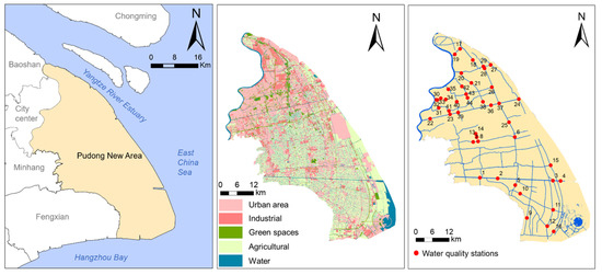
Figure 1.
Geographical location of the study area (left) and land use in Pudong New Area in 2010 (center) and spatial distribution of water quality monitoring stations (right).
2.2.2. Surface Water Quality
The surface water quality data were provided by Pudong New Area Environmental Protection Bureau, and all data originated from the monitoring stations of the surface water monitoring system in Pudong, covering different order of river and upstream and downstream reach; with continuous data of hydrological seasons for primary water quality indicators in 2010, a total of 44 monitoring stations were covered (Figure 1). The water quality indicators related to river pollution covers NH3-N, TP, TN, DO and CODMn, namely a total of six indicators was used in this study.
Compared with precipitation in the last decade, there was a clear distinction between the dry and wet seasons of that year; meanwhile, both the land use data and monthly water quality data of that year were collected by the authors, which is helpful to carry out the research of this paper’s topic. In order to reflect the seasonal variations of river water quality, according to the daily precipitation in Pudong New Area from January 2010 to December 2010, the entire monitoring period was divided into three periods: the dry season, the average season and the wet season. During the monitoring period, precipitation was higher in August and lower in January (Figure 2). Therefore, August was determined as the wet season, January was the dry season, and May was the average season.
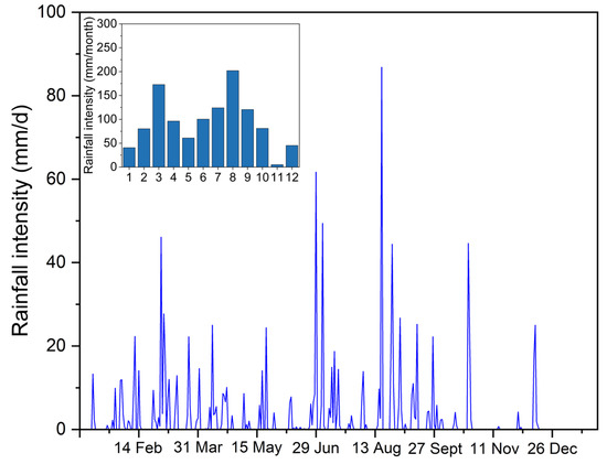
Figure 2.
Rainfall intensity in 2010.
2.3. Method
2.3.1. Hypothesis
- (i)
- The explanatory ability of land uses to the spatial variation of water quality is different in hydrological seasons, and the effect is greater in the wet season because the rainfall runoff effect is more significant, but lower in the dry season.
- (ii)
- Under different scales of hydrological response units, the explanatory ability of land use to the spatial variation of water quality is more complex. The effect should be small at the riparian scale, and the degree of influence can be increased with the enlarged scales.
2.3.2. Application of Hydrological Response Units
In order to determine the hydrologic unit of water quality monitoring stations, considering the features of the plain tidal area of Pudong New Area, the spatial scale is divided into: 50 m, 200 m, 500 m, 1000 m and 1500 m (Figure 3) [34,35]. Using the ArcGIS software, various radius buffers were considered taking the water quality monitoring stations as the center. After that, land use data of various buffers of each monitoring stations were acquired. Through the split operation in ArcGIS, the area of each land use in buffers was recalculated.
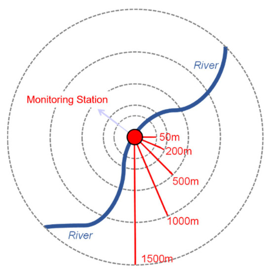
Figure 3.
Definition map of hydrological units in Pudong New Area. (A series of buffer zones—50 m, 200 m, 500 m, 1000 m and 1500 m—were created taking the water quality monitoring stations as the geographical center, and were considered as hydrological units for multi-scale analysis).
2.3.3. Redundancy Analysis (RDA)
Through Pearson’s correlation analysis, the general relationship between land use and water quality indicators can be determined. The advantage of RDA is that it can independently maintain the contribution of each variable to the variation of the dependent variable, neither simply analyzing the variable group, nor integrating several variables into a virtual complex variable (such as PCA), so that in the case of different combinations of explanatory variables, the single variable can still be described and the variable selection can be determined. As a method to determine the relationship between environmental quality and landscape indices, RDA has been widely accepted [36,37,38].
In the RDA ranking, if the angle between water quality parameters and land use types is less than 90 degrees, the two are positively correlated, and the water quality concentration will increase with the expansion of land use types; if the angle is greater than 90 degrees, the water quality parameters are negatively correlated with land use types, and the water quality concentration will decrease with the expansion of land use types. If the angle is equal to 90 degrees, indicating that the land use type and water quality parameters are completely vertical, there is no correlation. In addition, the length of the land use arrow in the ranking diagram indicates the comprehensive impact of land use on water quality. The longer the arrow, the higher the impact.
3. Results
3.1. Surface Water Quality of Different Hydrological Seasons
The water quality indicators varied in three hydrological seasons. The concentrations of CODMn and TN in the wet season are worse than those in the other two hydrological seasons, while that of NH3-N and TP in the average season is better (Figure 4). In general, the water quality is better in the average season but degraded in the wet season.
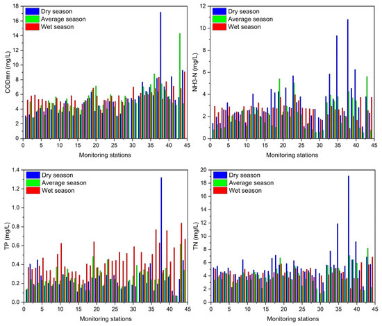
Figure 4.
Pollutant concentration of different hydrological seasons.
3.2. Pearson’s Correlation Analysis
3.2.1. Correlation among Surface Water Quality Indicators
Pearson’s correlation analysis was conducted on the water quality indicators using the dry, average, wet and annual means in 2010. The correlation test showed that (Table 1), there was a significant correlation between various water quality indicators, and there are obvious differences in three hydrological seasons.

Table 1.
Pearson’s correlation coefficient matrix among surface water quality indicators.
In the dry and average seasons, the correlation between water quality indicators is more obvious, while it is weak in the wet season. Among them, COD, BOD and NH3-N displayed the highest correlation coefficient with the other indicators, indicating that these indicators represented the main types of regional pollutants. pH and DO showed a lower correlation with the other indicators, indicating that they were relatively independent from the other indicators.
3.2.2. Correlation between Land Use and Water Quality
Pearson’s correlation of water quality and land use in 44 buffer zones was conducted (Table 2). The results showed that there was a strong relationship between urban areas and water quality indicators, while there was a negative correlation with DO and a positive correlation with TN and NH3-N. With an increase in buffer radius, the correlation between urban areas and DO increased and then decreased, but it remained stable for urban areas and TN and NH3-N.
Table 2.
Pearson’s correlation between water quality indicators (annual mean) and land use.
The correlation between water areas and water quality indicators is obviously better than other lands, that is, water quality could be better when the percentage of water areas is higher. Agricultural land has a positive correlation with pH and DO, but a negative correlation with NH3-N and TN; and with the increase in buffer radius, the impact on water quality grew. Industrial land and green spaces only correlated with BOD and CODMn at smaller scales, and there was almost no correlation with other water quality indicators.
3.3. RDA on the Relationship
To quantify the effects of land use and hydrological seasons under spatial changes in water quality, Canoco 4.5 software was used for RDA. Taking six water quality indicators as species variables and five land use variables as environment variables, the relationship between different land use and water quality indicators was conducted.
In order to identify the land use variables of the spatial variation of water quality in Pudong New Area, a variable screening process based on Monte Carlo Permutation method was used in the operation to progressively identify significant variables (499 non-restricted screening cycles). On this basis, the engine value of the RDA axis, the correlation coefficient between land use variables and the ranking axis, and the explanatory ability of each land use to the spatial variation of surface water quality were obtained. It can be seen that the correlation between different water quality indicators and land use changed with scale, and there were certain differences between different hydrological seasons (Figure 5).

Figure 5.
RDA of surface water quality by land use at different hydrological seasons and scales in Pudong New Area, Shanghai.
The results of the full model RDA considering all land use variables showed that, in the dry season, with the expansion of buffer zone, the explanatory ability of land use also increased, but the change was minimal. When the radius was smaller than 200 m, the explanatory ability was greater than 23%. When the radius was 500 m, it was reduced to 20.7%. Finally, when the radius of the buffers increased to 1500 m, the explanatory ability increased to greater than 25%. It can be considered that with the increase in spatial scale, the above five land use types had a curved change in the ability to explain water quality variation, and the optimal scale is approximately 1000 m.
In the average season, the larger the buffer zone, the less likely the proportion of land use can explain the spatial variations of water quality. When the radius is less than 500 m, the explanatory ability is approximately 40%. When it increased to 1000 m, the explanatory ability began to be less than 35%. It can be considered that with the increase in the scale, the above five land use types have a curved change in the ability to explain water quality, and the optimal scale maybe approximately 500 m.
During the wet season, land use variables can better explain the spatial variation of water quality with the increase in buffer radius, and this then tends to be stable. When the radius of the buffer increased from 50 m to 500 m, the explanatory ability of land use variables increased from 15.1% to 25%. However, when the buffer increased to the maximum scale of 1500 m, it only decreased slightly from 25.0% to 23.6%. It can be deduced that as the scale increased, the explanatory ability of land use would gradually stabilize.
For the annual mean situation, the proportion of land use variables in each radius buffer space unit to explain the spatial differentiation of water quality is almost more than 30%, and there is no obvious fluctuation.
4. Discussions
4.1. Difference of Spatial Effect of Land Uses
Total explanatory ability of land use to water quality in the study area is approximately 30%, and there are differences in various buffers (Figure 6). Different land uses showed a scale effect on the spatial variation of surface water quality. Urban areas and agricultural land are the most significant variables. The explanatory ability of urban areas is negatively correlated with buffer radius, but the relationship between agricultural land is positive correlated. That of water areas, industrial land and green spaces are more complicated (Table 2).
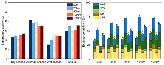
Figure 6.
Explanatory ability of RDA of water quality response to land use (left). Correlation between land use and river water quality in different hydrological seasons (A: dry season, B: average season, C: wet season, and D: annual) (right).
At the 50 m radius, in all hydrological seasons, urban areas, agricultural land and water areas displayed a higher explanatory ability on water quality at this riparian zone. The explanatory ability of urban areas in the average season is even as high as 24%, indicating that at a smaller scale, urban areas, agricultural land and water areas were the major drivers affecting water quality. Therefore, reasonable arrangement of riparian area, agricultural land and water areas is of great significance to improve river quality.
Within the radius from 200 to 1500 m, the impact of urban areas on water quality decreased significantly, while the impact of agricultural land and water areas increased rapidly. Therefore, with the increase in spatial scale, the area of water areas gradually increases, and the explanatory ability also rises sharply. This also showed that protecting the waters at a larger scale is also one of the effective measures to prevent the deterioration of river quality. However, when the buffer radius is greater than 1000 m, the explanatory ability of water quality of water areas does not increase further and remains stable or decreases slightly.
The explanatory ability of agricultural land increases with the expansion of buffers, which may be related to farmland management measures. The reasons may be related to farming methods, pesticide and fertilizer utilization, irrigation and other farmland measures, as well as the area of cultivated land, the distance from the receiving water, topography and so on [15].
The relationship between other land uses and water quality is relatively complex. For example, when the buffer radius is within 50 m, green spaces is negatively correlated, but when the buffer radius is increased, it gradually changes to a positive correlation, which indicated that the riparian green spaces have a certain effect on purifying rivers, but the enlarged area of green spaces beyond 500 m may be unfavorable to river water quality. This is because the riparian green spaces within 500 m are mostly natural green spaces, which is less affected by human activities and plays a certain pollutant interception effect. The green spaces far from riverbank are mostly composed of artificial lawns, which are generally scattered among urban areas. Affected by urban human activities and urban surface runoff, its pollutant load is often higher, thus showing a positive effect on the river quality [39].
4.2. Differences in Various Hydrological Seasons
In three hydrological seasons, the total explanatory rate of land use is quite different, which is 25% in the dry season, 40% in the average season, 20% in the wet season, and 30% in annual condition. Therefore, the explanatory ability of land use to water quality is the largest in the average season, but smaller in the dry season and the wet season. In particular, in the wet season, unexpectedly, the correlation between land use and water quality is not as strong as that in the average and even the dry season, and the explanatory ability of land use is only approximately 20%. There was also no significant impact regarding urban areas.
There are also obvious differences among different types of land in different hydrological seasons. In the dry season and the wet season, the explanatory ability of urban areas and water areas is the strongest, while that of other land uses is weak. In the average season, the explanatory ability of all land uses increased compared with the dry and wet seasons, and agricultural land had the most significant increase in explanatory ability to water quality. In the summary, urban areas, agricultural land and water areas have the strongest ability to explain water quality.
On the whole, in the dry season and the wet season, the explanatory ability of urban areas, agricultural land and water areas is weaker than in the average season, while the explanatory ability of green spaces is obviously stronger than in the average season. The explanatory ability of land use to water quality is the largest in the average season, but smaller in the dry season and the wet season.
4.3. Comparison with the Hypothesis
In general, land uses can mostly explain the spatial variation of water quality in the average season, while it is smallest in the wet season (Figure 6). In the dry season, there were few rainfall events and rainfall runoff, which met the expectation. However, this was contrary to common sense in the wet season. A possible cause of this situation is that the sewage brought by a lot of rain pollution mixed with the sewage pipe network is discharged into the rainfall runoff, resulting in poor river water quality, and the relationship between land use and water quality is disturbed and thus weak [40,41].
Compared with the hypothesis, total explanatory ability in RDA of land use to water quality in the study area is approximately 30%, and there is little difference in various buffers (Figure 6). Different land use showed complex scale effects on the spatial variation of surface water quality.
4.4. Limitations
This study used statistics for analysis. In the process of studying the impact of land use on surface water quality in different hydrological periods, there was a lack of research on upstream water quality, bioactive surface permeability and its differences, natural surface runoff changes caused by urban drainage systems, river bottom sediment re-suspension, and air temperature. The infiltration coefficient and runoff coefficient of different land use modes need to be simulated by MIKE and other hydrological models [34,42].
5. Conclusions
The purpose of this study was to determine the relationship between land use and water quality, and how buffer ranges and hydrological seasons affect this relationship. In Pudong New Area of Shanghai, the contribution of land use to the spatial variation of water quality is approximately 30%, and land uses displayed the largest explanatory ability in the average season, but this was significantly lower in the wet and dry seasons. Moreover, in the dry and wet seasons, the explanatory ability of urban, agricultural land and water areas was weaker than in the average season, while this was obviously stronger in the green spaces than in the average season. Different land uses showed a scale effect on the spatial variation of surface water quality. At a smaller scale, urban, agricultural land and water areas were the major factors affecting water quality. When the radius changed from 500 to 1500 m, the impact of urban areas on water quality decreased significantly, while the impact of agricultural land and water areas increased rapidly. When the buffer is within 50 m, green space is negatively correlated, but when the buffer radius increases, it gradually changes to a positive correlation. This study is expected to provide references for future decision making of urban construction, rainfall pollution control, and environmental planning and management.
Author Contributions
Conceptualization, D.W. and G.H.; methodology, X.Z.; software, D.W.; validation, H.D., H.W. and Z.Z.; formal analysis, D.L.; investigation, J.Z.; resources, X.Z.; data curation, Z.Z.; writing—original draft preparation, D.W.; writing—review and editing, D.W.; visualization, J.Z.; supervision, J.Z.; project administration, J.Z.; funding acquisition, J.Z. All authors have read and agreed to the published version of the manuscript.
Funding
This study was funded by the Shanghai Water Environment Simulation and Water Ecological Restoration Engineering Technology Research Center (WESER-202206).
Data Availability Statement
No new data was created or analyzed in this study. Data sharing is not applicable to this article.
Conflicts of Interest
The authors declare no conflict of interest.
References
- Batbayar, G.; Pfeiffer, M.; Kappas, M.; Karthe, D. Development and application of GIS-based assessment of land-use impacts on water quality: A case study of the Kharaa River Basin. AMBIO 2018, 48, 1154–1168. [Google Scholar] [CrossRef]
- Carroll, S.; Liu, A.; Dawes, L.; Hargreaves, M.; Goonetilleke, A. Role of Land Use and Seasonal Factors in Water Quality Degradations. Water Resour. Manag. 2013, 27, 3433–3440. [Google Scholar] [CrossRef]
- Hanna, D.E.L.; Lehner, B.; Taranu, Z.E.; Solomon, C.T.; Bennett, E.M. The relationship between watershed protection and water quality: The case of Québec, Canada. Freshw. Sci. 2021, 40, 382–396. [Google Scholar] [CrossRef]
- Qiu, Z.; Hall, C.; Drewes, D.; Messinger, G.; Prato, T.; Hale, K.; Van Abs, D. Hydrologically Sensitive Areas, Land Use Controls, and Protection of Healthy Watersheds. J. Water Resour. Plan. Manag. 2014, 140, 04014011. [Google Scholar] [CrossRef]
- Wang, L.; Wang, S.; Zhou, Y.; Zhu, J.; Zhang, J.; Hou, Y.; Liu, W. Landscape pattern variation, protection measures, and land use/land cover changes in drinking water source protection areas: A case study in Danjiangkou Reservoir, China. Glob. Ecol. Conserv. 2019, 21, e00827. [Google Scholar] [CrossRef]
- Cheng, P.; Meng, F.; Wang, Y.; Zhang, L.; Yang, Q.; Jiang, M. The Impacts of Land Use Patterns on Water Quality in a Trans-Boundary River Basin in Northeast China Based on Eco-Functional Regionalization. Int. J. Environ. Res. Public Health 2018, 15, 1872. [Google Scholar] [CrossRef]
- Fan, K.; Pei, W.J.; Zhang, J.S.; Yu, J.X.; Zeng, W.J. Analysis on landscape pattern of land use and eco- environment characteristics of three lake basins in yunnan province, china. Appl. Ecol. Environ. Res. 2018, 16, 5693–5704. [Google Scholar] [CrossRef]
- Cui, H.; Zhou, X.; Guo, M.; Wu, W. Land use change and its effects on water quality in typical inland lake of arid area in China. J. Environ. Biol. 2016, 37, 603–609. [Google Scholar]
- Xia, L.L.; Liu, R.Z.; Zao, Y.W. Correlation Analysis of Landscape Pattern and Water Quality in Baiyangdian Watershed. In Proceedings of the 18th Biennial ISEM Conference on Ecological Modelling for Global Change and Coupled Human and Natural Systems, Beijing, China, 20–23 September 2011; Beijing Normal University: Beijing, China, 2011; pp. 2188–2196. [Google Scholar]
- Xu, F.; Bao, H.X.; Li, H.; Kwan, M.-P.; Huang, X. Land use policy and spatiotemporal changes in the water area of an arid region. Land Use Policy 2016, 54, 366–377. [Google Scholar] [CrossRef]
- Bai, X.; Shen, W.; Wang, P.; Chen, X.; He, Y. Response of Non-point Source Pollution Loads to Land Use Change under Different Precipitation Scenarios from a Future Perspective. Water Resour. Manag. 2020, 34, 3987–4002. [Google Scholar] [CrossRef]
- Gong, D.; Hong, X.; Zeng, G.; Wang, Y.; Zuo, S.; Liu, X.; Wu, J. Prediction of Water Quality in Rivers in Agricultural Regions Typical of Subtropics in China Using Multivariate Linear Regression Model. J. Ecol. Rural. Environ. 2017, 33, 509–518. [Google Scholar]
- Pan, Y.; Yu, D.; Wang, X.; Xu, Z.C.; Wang, X.Y. Prediction of Land Use Landscape Pattern Based on CA-Markov Model. Soils 2018, 50, 391–397. [Google Scholar]
- Dunn, S.M.; Sample, J.; Potts, J.; Abel, C.; Cook, Y.; Taylor, C.; Vinten, A.J.A. Recent trends in water quality in an agricultural catchment in Eastern Scotland: Elucidating the roles of hydrology and land use. Environ. Sci. Process. Impacts 2014, 16, 1659–1675. [Google Scholar] [CrossRef]
- Zhang, M.-S.; Li, W.; Zhang, W.-G.; Li, Y.-T.; Li, J.-Y.; Gao, Y. Agricultural land-use change exacerbates the dissemination of antibiotic resistance genes via surface runoffs in Lake Tai Basin, China. Ecotoxicol. Environ. Saf. 2021, 220, 112328. [Google Scholar] [CrossRef] [PubMed]
- Herlihy, A.T.; Stoddard, J.L.; Johnson, C.B. The Relationship between Stream Chemistry and Watershed Land Cover Data in the Mid-Atlantic Region, U.S. Water Air Soil Pollut. 1998, 105, 377–386. [Google Scholar] [CrossRef]
- Galbraith, L.M.; Burns, C.W. Linking Land-use, Water Body Type and Water Quality in Southern New Zealand. Landsc. Ecol. 2006, 22, 231–241. [Google Scholar] [CrossRef]
- Clune, J.W.; Crawford, J.K.; Chappell, W.T.; Boyer, E.W. Differential effects of land use on nutrient concentrations in streams of Pennsylvania. Environ. Res. Commun. 2020, 2, 115003. [Google Scholar] [CrossRef]
- Gorgoglione, A.; Gregorio, J.; Ríos, A.; Alonso, J.; Chreties, C.; Fossati, M. Influence of Land Use/Land Cover on Surface-Water Quality of Santa Lucía River, Uruguay. Sustainability 2020, 12, 4692. [Google Scholar] [CrossRef]
- Chen, D.; Elhadj, A.; Xu, H.; Xu, X.; Qiao, Z. A Study on the Relationship between Land Use Change and Water Quality of the Mitidja Watershed in Algeria Based on GIS and RS. Sustainability 2020, 12, 3510. [Google Scholar] [CrossRef]
- de Mello, K.; Taniwaki, R.H.; de Paula, F.R.; Valente, R.A.; Randhir, T.O.; Macedo, D.R.; Leal, C.G.; Rodrigues, C.B.; Hughes, R.M. Multiscale land use impacts on water quality: Assessment, planning, and future perspectives in Brazil. J. Environ. Manag. 2020, 270, 110879. [Google Scholar] [CrossRef]
- Xu, S.; Li, S.-L.; Zhong, J.; Li, C. Spatial scale effects of the variable relationships between landscape pattern and water quality: Example from an agricultural karst river basin, Southwestern China. Agric. Ecosyst. Environ. 2020, 300, 106999. [Google Scholar] [CrossRef]
- Fang, N.; Liu, L.-L.; You, Q.-H.; Tian, N.; Wu, Y.-P.; Yang, W.-J. Effects of Land Use Types at Different Spatial Scales on Water Quality in Poyang Lake Wetland. Huan Jing Ke Xue=Huanjing Kexue 2019, 40, 5348–5357. [Google Scholar] [PubMed]
- Deng, X. Influence of water body area on water quality in the southern Jiangsu Plain, eastern China. J. Clean. Prod. 2020, 254, 120136. [Google Scholar] [CrossRef]
- Álvarez-Cabria, M.; Barquín, J.; Peñas, F.J. Modelling the spatial and seasonal variability of water quality for entire river networks: Relationships with natural and anthropogenic factors. Sci. Total Environ. 2016, 545–546, 152–162. [Google Scholar] [CrossRef]
- Yu, X.; Hawley-Howard, J.; Pitt, A.L.; Wang, J.-J.; Baldwin, R.F.; Chow, A.T. Water quality of small seasonal wetlands in the Piedmont ecoregion, South Carolina, USA: Effects of land use and hydrological connectivity. Water Res. 2015, 73, 98–108. [Google Scholar] [CrossRef] [PubMed]
- Xu, J.; Liu, R.; Ni, M.; Zhang, J.; Ji, Q.; Xiao, Z. Seasonal variations of water quality response to land use metrics at multi-spatial scales in the Yangtze River basin. Environ. Sci. Pollut. Res. 2021, 28, 37172–37181. [Google Scholar] [CrossRef]
- Li, G.Y.; Li, L.Z.; Kong, M. Multiple-Scale Analysis of Water Quality Variations and Their Correlation with Land use in Highly Urbanized Taihu Basin, China. Bull. Environ. Contam. Toxicol. 2020, 106, 218–224. [Google Scholar] [CrossRef]
- Vogt, R.J.; Frost, P.C.; Nienhuis, S.; Woolnough, D.A.; Xenopoulos, M.A. The dual synchronizing influences of precipitation and land use on stream properties in a rapidly urbanizing watershed. Ecosphere 2016, 7, e01427. [Google Scholar] [CrossRef]
- Wang, J.; Hou, L.; He, X.; Liu, T.; Deng, Y. Land Use Change and Its Eco-environmental Effects in Urban Agglomeration of Chengdu Plain During 2000–2019. Bull. Soil Water Conserv. 2022, 42, 360–368. [Google Scholar]
- Zhao, W.; Zhu, X.; Sun, X.; Shu, Y.; Li, Y. Water quality changes in response to urban expansion: Spatially varying relations and determinants. Environ. Sci. Pollut. Res. 2015, 22, 16997–17011. [Google Scholar] [CrossRef]
- Zhou, X.; Zhang, W.; Pei, Y.; Jiang, X.; Yang, S. Zoning Strategy for Basin Land Use Optimization for Reducing Nitrogen and Phosphorus Pollution in Guizhou Karst Watershed. Water 2022, 14, 2589. [Google Scholar] [CrossRef]
- Wang, J.; Zhang, J.; Xiong, N.; Liang, B.; Wang, Z.; Cressey, E.L. Spatial and Temporal Variation, Simulation and Prediction of Land Use in Ecological Conservation Area of Western Beijing. Remote. Sens. 2022, 14, 1452. [Google Scholar] [CrossRef]
- Wang, Z.; Zhang, S.; Peng, Y.; Wu, C.; Lv, Y.; Xiao, K.; Zhao, J.; Qian, G. Impact of rapid urbanization on the threshold effect in the relationship between impervious surfaces and water quality in shanghai, China. Environ. Pollut. 2020, 267, 115569. [Google Scholar] [CrossRef] [PubMed]
- Zhao, J.; Lin, L.; Yang, K.; Liu, Q.; Qian, G. Influences of land use on water quality in a reticular river network area: A case study in Shanghai, China. Landsc. Urban Plan. 2015, 137, 20–29. [Google Scholar] [CrossRef]
- Dou, J.; Xia, R.; Chen, Y.; Chen, X.; Cheng, B.; Zhang, K.; Yang, C. Mixed spatial scale effects of landscape structure on water quality in the Yellow River. J. Clean. Prod. 2022, 368, 133008. [Google Scholar] [CrossRef]
- Li, S.; Zhang, J.; Jiang, P.; Zhang, L. Linking land use with riverine water quality: A multi-spatial scale analysis relating to various riparian strips. Front. Environ. Sci. 2022, 10, 1013318. [Google Scholar] [CrossRef]
- Wang, N.; Xiong, J.; Wang, X.C.; Zhang, Y.; Liu, H.; Zhou, B.; Pan, P.; Liu, Y.; Ding, F. Relationship between phytoplankton community and environmental factors in landscape water with high salinity in a coastal city of China. Environ. Sci. Pollut. Res. 2018, 25, 28460–28470. [Google Scholar] [CrossRef]
- Neill, C.; Deegan, L.A.; Thomas, S.M.; Cerri, C.C. Deforestation for pasture alters nitrogen and phosphorus in small Amazonian Streams. Ecol. Appl. 2001, 11, 1817–1828. [Google Scholar] [CrossRef]
- Xu, Z.; Xu, J.; Yin, H.; Jin, W.; Li, H.; He, Z. Urban river pollution control in developing countries. Nat. Sustain. 2019, 2, 158–160. [Google Scholar] [CrossRef]
- Yin, H.; Xie, M.; Zhang, L.; Huang, J.; Xu, Z.; Li, H.; Jiang, R.; Wang, R.; Zeng, X. Identification of sewage markers to indicate sources of contamination: Low cost options for misconnected non-stormwater source tracking in stormwater systems. Sci. Total. Environ. 2018, 648, 125–134. [Google Scholar] [CrossRef]
- Shi, Y.; Yao, Y.; Zhao, J.; Li, X.; Yu, J.; Qian, G. Changes in Reticular River Network under Rapid Urbanization: A Case of Pudong New Area, Shanghai. Water 2022, 14, 523. [Google Scholar] [CrossRef]


Disclaimer/Publisher’s Note: The statements, opinions and data contained in all publications are solely those of the individual author(s) and contributor(s) and not of MDPI and/or the editor(s). MDPI and/or the editor(s) disclaim responsibility for any injury to people or property resulting from any ideas, methods, instructions or products referred to in the content. |
© 2023 by the authors. Licensee MDPI, Basel, Switzerland. This article is an open access article distributed under the terms and conditions of the Creative Commons Attribution (CC BY) license (https://creativecommons.org/licenses/by/4.0/).