Article

Overflow Capacity Prediction of Pumping Station Based on Data Drive

Beijing International Collaboration Base on Brain Informatics and Wisdom Services, Beijing 100124, China
*
Author to whom correspondence should be addressed.
Water 2023, 15(13), 2380; https://doi.org/10.3390/w15132380
Submission received: 25 April 2023 / Revised: 16 June 2023 / Accepted: 26 June 2023 / Published: 28 June 2023

Abstract

:
In recent years, the information requirements of pumping stations have become higher and higher. The prediction of overflow capacity can provide important reference for flood carrying capacity, water resource scheduling and water safety. In order to improve the accuracy, stability and generalization ability of the model, a BiGRU–ARIMA data-driven method based on self-attention mechanism is proposed to predict the flow capacity of the pump station. Bidirectional gated recurrent unit (BiGRU), a variant of cyclic neural network (RNN), can not only deal with nonlinear components well, but also deal with the problem of insufficient dependence over long distances and has a simple structure. Autoregressive integrated moving average (ARIMA) has the advantage of being sensitive to linear components. Firstly, the characteristics of the pre-processed pump station data are selected and screened through Pearson correlation coefficient and a self-attention mechanism. Then, a bi-directional gated recurrent unit (BiGRU) is used to process the nonlinear components of the data, and a dropout layer is added to avoid overfitting phenomena. We extract the linear features of the obtained error terms using the ARIMA model and use them as correction items to correct the prediction results of the BiGRU model. Finally, we obtain the prediction results of the overflow and water level. The variation characteristics of overdischarge are analyzed by the relation of flow and water level. In this paper, the actual production data of a Grade 9 pumping station of Miyun Reservoir is taken as an example to verify the validity of the model. Model performance is evaluated according to mean absolute error (MAE), mean absolute percentage error (MAPE) and linear regression correlation coefficient (R2). The experimental results show that, compared with the single ARIMAX, BiGRU model and BP neural network, the SA–BiGRU–ARIMA hybrid prediction model has a better prediction effect than other data-driven models.

1. Introduction

At present, the main causes of Earth’s water crisis are water resources pollution, uneven distribution of water resources and waste of water resources. Pumping stations have regional functions of water transfer, water supply, flood control and waterlogging, which can solve the problems of uneven distribution and waste of water resources to a certain extent [1,2]. The unique advantage of developing a pump station is that it is less affected by environmental and resource factors such as terrain and water source. The disadvantages are mainly reflected in the lack of intelligent means of pump station equipment, and the semi-mechanical and semi-artificial control results in a greater influence by staff. Overcurrent capacity is an important index to measure the flood control capacity of river course [3]. Real-time overflow capacity prediction can not only provide a scientific decision-making basis for water safety and flood control, but also help pump station staff to grasp the dynamic changes of water level and flow earlier to prevent the occurrence of disasters in time. Therefore, it is an important means to establish a scientific and effective forecast model for the flow capacity of pump stations to improve the intelligence level of pump stations.
At present, the prediction models of flow capacity are mainly one-dimensional and two-dimensional hydraulic physical models. Naito et al. [4] is based on the physical river channel, Suzhen et al. [5] is based on the automatic adjustment principle of the river bed, and the flat beach discharge is taken as the index to predict the overflow capacity. Hermann divided water flow into four different forms, according to water conservancy characteristics through the length of the dam crest and different water levels, and conducted a detailed study on the overcurrent capacity [6]. Yang et al. [7] and Chen et al. [8] predicted the relationship between water level and discharge by numerical simulation. Zheng et al. [9], Bijankhan et al. [10] and Fencl M et al. [11] established the overflow calculation formula. Timbadiya [12], Karim et al. [13] built a simulation of river flow capacity through hydraulic engineering software. All of these methods are based on hydrodynamic models and rely too much on physical models. However, the internal structure of physical models is complex and the calculation is time-consuming, which will cause high load calculation problems in the process of parameter calibration, multi-scenario analysis and decision optimization, which greatly limits its application value.
In addition, the existing channel is designed according to the standard interface, and the (mathematical/physical) model and parameters (river width, depth, number of gates) are fixed. Moreover, during the long-term operation of the pump station, the river channel will produce siltation, water grass, etc., and there may be errors in the original design parameters, which will lead to the deviation of the expected effect in the flood control dispatching process. Furthermore, in the operation process of the cascade pump station, it is necessary to consider the contact between adjacent pump stations. Therefore, a data-driven approach is proposed, and the design of the model mainly depends on the input and output data, without the need for an explicit mathematical model [14].
The main existing data-driven methods include ARIMA [15], support vector machine (SVM) [16], random forest (RF) [17], artificial neural network (ANN) [18], recurrent neural network (RNN) [19], etc. For example, Yan et al. [20] and Yong et al. [21] used a BP neural network model to predict overflow. Wei-CC et al. used multi-layer perceptron (MLP) to predict the required pump flow rate and use tree derived rules obtained from correlation classifiers to predict the optimal pump combination [22]. Random forest and Bayesian models are used to predict river level and discharge [23,24,25]. Tan used the ARIMAX model to model sewer flow, and made reliable predictions of flow 2 h in advance through recursive estimation parameters of each time step by the least square method [26]. Musarat et al. used ARIMA analysis and prediction model to forecast river discharge [27]. Pierini verified ANN’s excellent performance in predicting or supplementing daily flow [28]. Xu W successfully applied long short-term memory (LSTM) to the prediction of 10-day average flow and daily average flow [29]. Aryal used the conversion of stream flow data for system model calibration [30].
Single models have the problems of low prediction accuracy and large residual error. Therefore, a combination model is proposed. By combining a linear model and nonlinear model or a traditional model and machine learning model, the prediction effect of the model can be improved to a certain extent. Li Y et al. proposed a LSTM training method based on attention mechanism to predict multivariate time series [31]. Li X et al. proposed a CNN–LSTM river flow prediction model, which effectively solved the problem of diversity reduction in depth networks [32]. Zhang combined the advantages of complete ensemble empirical mode decomposition with adaptive noise and BiLSTM (CEEMDAN–BiLSTM) to predict flow in the middle and lower reaches of the Yellow River and verified the effectiveness of bidirectional recurrent neural networks in terms of traffic prediction [33]. Liang et al. adopted the improved the BiGRU model with the introduction of attention mechanism to achieve the high-precision prediction of the discharge during the 36 h prediction period [34]. Chen et al. used a graph attention–recurrent neural network (GA–RNN) prediction model based on graph attention mechanism to predict flood peak and flood arrival time in flood season [35]. In conclusion, RNN and its variants have better performance in river flow prediction. BIGRU not only has a simple structure but can also solve the gradient disappearance and explosion problems of the traditional RNN, while the ARIMA model can compensate for its insensitivity to linear components. In addition, the innovative and improved RNN network and ARIMA combination algorithm has not been applied to the study of overflow characteristics of pumping stations.
Based on the correlation between pump station information and multivariable time series data, a BiGRU–ARIMA prediction model based on self-attention mechanism is proposed. First, isolated forest, K-nearest neighbor method and Pearson correlation coefficient are used to preprocess the data; then, the AT–BiGRU model is used for preliminary prediction of nonlinear components and the error terms are modified by an ARIMA model. Finally, the model is evaluated according to mean absolute error (MAE), mean absolute percentage error (MAPE) and linear regression correlation coefficient (R2). This paper takes Qianliulin Pumping station of Miyun Reservoir as an example to predict the flow capacity. Then, ARIMAX, BiGRU and BP neural network models are used for a comparison experiment, and model evaluation is carried out to verify the effectiveness and superiority of the AT–BiGRU–ARIMA model.

2. Materials and Methods

2.1. Study Areas and Monitor Data

Miyun Reservoir regulation and storage project is a large-scale cascade diversion project. Water taken from Tuancheng Lake is lifted and fed to Huairou Reservoir from Tundian Pumping Station, Qianliulin Pumping Station, Niantou Pumping Station, Xingshou Pumping Station, Lishishan Pumping Station and Xidaishang Pumping Station. After the water of Huairou Reservoir is returned to the water refill source, it is lifted from Guojiawu Pumping Station to the inverted siphon of Beitai upper through Jingmi Diversion Canal. After being pressurized by Yanqi Pump Station and Xiwengzhuang Pump Station, the water is pressurized into Miyun Reservoir. The total length of the line is 103 km with a total head of 132.85 m. It is not only a key project of the South-to-North Water diversion project, but also an important guarantee of water safety in Beijing.
The flow and water level of the cascade pump stations are closely connected. The variation of discharge under characteristic water level is an important index to measure the river’s overflow capacity [36,37]. Therefore, the data of Tundian Pumping Station and Qianliulin Pumping station are selected to predict realize the prediction of the flow capacity of Qianliulin Pumping station. The two pumping stations are 9.5 km apart, and the flow conditions are very complicated, making it difficult to predict, as shown in Figure 1. In this paper, the cumulative flow of QianLiulin pump station gate is used as the index to analyze the flow capacity. The monitoring data of Tundian Pumping Station and Qianliulin Pumping Station for 12 months in 2020 were selected. Data are collected every minute by sensors deployed in various pieces of equipment at the pump station. The data include: rear pool water level (TB-WL), gate cumulative flow rate (TGate-AF1), unit instantaneous flow rate (TUnit-IF1), pump frequency (TPump-Fre1), pipeline pressure (TPP1) of Tundian Pumping Station, and front pool water level (QF-WL), gate cumulative flow rate (QGate-AF), unit of QianLiulin Pump Station instantaneous flow rate (QUnit-IF2), pump frequency (qpum-fre2) and pipeline pressure (QPP2). The information and statistical characteristics for these data are shown in Table 1.

2.2. Monitoring Aata Cleaning and Interpolation

The data used in this paper are collected by different types of sensors equipped with different equipment in the pumping station, which may be affected by equipment failure, weather changes, human input errors or abnormal events, leading to the occurrence of some outliers. Ignoring these outliers may lead to conclusive errors in the training model. Therefore, in order to ensure the accuracy of model prediction, the data must be cleaned to optimize the detection model.
For duplicate samples, this paper retains the value of the first sample and deletes the remaining duplicate samples according to timestamp order.
For abnormal samples, this paper adopts the isolated forest algorithm to process the data samples. Isolated forest is an unsupervised anomaly detection method applicable to continuous numerical data [38]. The outliers in the data samples are removed by the isolated forest algorithm. An isolated forest is composed of several binary trees. By randomly selecting features from a given feature set and then randomly selecting a segmentation value between the maximum and minimum values of the feature to isolate outliers, outliers have a short tree path and are easy to isolate, while normal values need to be divided many times to be isolated. The implementation process is shown in Figure 2.
  • Randomly select n data from the data sample as a sub-sample, with a maximum value of x m a x and a minimum value of x m i n , to put in the root node of the i-tree.
  • A dimension is randomly selected, and a cut point p is randomly selected from the current node data, x m i n p x m a x .
  • The current node data are divided into 2 sections by cutting point p, putting data smaller than p in the selected dimensions in the left subtree of the current node, and data larger than p in the selected dimensions in the right subtree of the current node.
  • Repeat steps 1 to 3 recursively on the next node until only one datum exists on each node or the maximum growth height of the tree is reached.
  • Select the next binary tree and repeat steps 1 to 4 until all the binary tree training is complete.
  • Calculate the average path length for each isolated tree c ( n ) ,
c n = 2 H n 1 2 n 1 n
where, n is the number of samples, x is the test samples, and H ( i ) is the harmonic number, can be estimated as ln i + ξ (euler’s constant = 0.577215664) and the path length h ( x ) (expect E ( h ( x ) ) ), Finally by E ( h ( c ) ) for samples of abnormal quantile s ( x , n ) , namely,
s x , n = 2 E h x c n
where, 0 s ( x , n ) 1 . The closer the value is to 1, the higher the possibility that it is an anomaly; the closer the value is to 0, the higher the possibility that it is a normal point. If the scores of all data are close to 0.5, it can be considered that there is no anomaly in the data.
Since the pump station data used in this paper are characterized by time continuity, the N-nearest neighbor method is adopted to fill in the missing data. Firstly, the n samples closest to the missing sample were determined according to Euclidean distance, and the weighted average of these n values is used to estimate the missing data of the sample. The specific calculation formula is as follows:
d x , y = x 1 y 1 2 + x 2 y 2 2 + + x n y n 2 = i = 1 n x i y i 2
h N = i = 1 n h i n
h i ( i = 1,2 , . . . , n ) is the selected adjacent n data points; h N is the final fill data.

2.3. Variable Selection: Pearson Correlation Coefficient

Pearson correlation coefficient and random sampling are both good methods for variable selection. However, sampling mainly focuses on small group samples for analysis, using small sample sampling to estimate the characteristics of the overall sample, which is not comprehensive. Moreover, the selection of variables in equal probability sampling is also random. Therefore, for continuous and linearly correlated sequences, the combination of Pearson correlation coefficient and sampling is the most suitable method. The sequence can be sampled equidistantly to reduce the number of data; then, the Pearson correlation coefficient can be used to calculate the sequence correlation.
Pearson correlation coefficient can effectively measure the degree of fit between two random variables. It is a linear correlation coefficient with a value between −1 and 1. The larger the absolute value, the stronger the correlation; the smaller the absolute value, the weaker the correlation. The value range [0.8, 1.0] indicates strong correlation, the value range [0.5, 0.8] indicates a moderate degree of correlation and [0.0, 0.5] indicates that the correlation is not high. ρ x y is used to denote the Pearson correlation coefficient, defined as follows:
ρ x y = C O V X , Y σ x σ y = E X Y E X E Y E x 2 E 2 X E Y 2 E 2 Y = i = 1 n x i x y i y i = 1 n x i x 2 i = 1 n y i y 2
X and Y are random variables; c o v ( X , Y ) is the covariance of X and Y; σ x , σ y , is the standard deviation of X and Y; x , y , is the mean of X and Y.

2.4. Bidirectional Gated Recurrent Unit

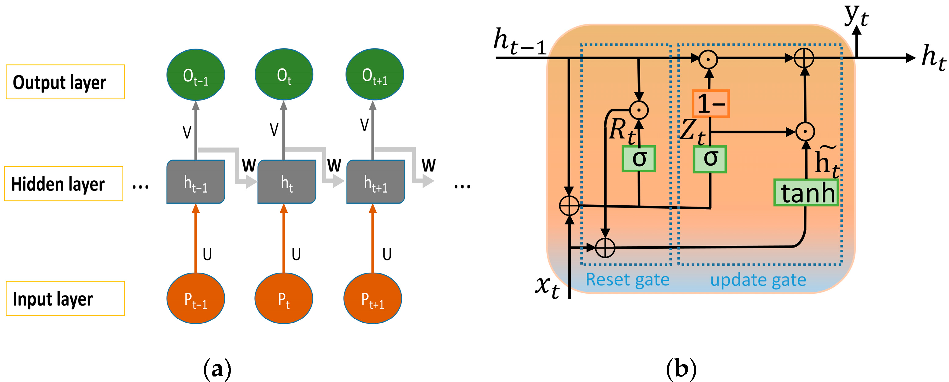
Neural networks have excellent nonlinear data learning ability, among which cyclic neural networks (RNN) can process time series data well, collect information contained in input sequence continuously from the front to the back and mine the internal connection of data. The RNN infrastructure consists of an input layer p t , hidden layer h t , output layer o t , corresponding weight matrix W and bias of item b [39]. The basic structure is shown in Figure 3a. Although RNN can realize the extraction of historical information features of the target state, it is easy to cause gradient disappearance and explosion in the training process because the back propagation path is too long.
Both LSTM and GRU, as variants of RNN, overcome the gradient disappearance and gradient explosion problems existing in traditional RNNs through gated cycle units. Although LSTM can optimize the model training problem, it also has the problem of an excessive number of model parameters and complicated calculation. On the basis of LSTM, GRU simplifies the gated cycle unit and uses two gates—update gate and reset gate—to control and update parameter information, reducing the number of parameters and achieving experimental results similar to LSTM [40]. The GRU model structure is shown in Figure 3b.
The update gate R t determines the amount of previous memory saved to the current time step. The larger the threshold, the greater the role of the previous information in the current status information. The reset gate Z t determines how to combine the new input with the previous memory. The lower the threshold, the less information is forgotten. The computational structure of the model is as follows:
R t = σ x t w x r + h t 1 w h r + b r
Z t = σ x t w x z + h t 1 w h z + b z
h t ~ = t a n h x t w x h + h t 1 R t w h h + b h
h t = 1 Z t h t 1 + Z t h t ~
y t = σ w y y h t + b y
x t is the input of the current time; h t 1 is the state of the hidden layer at the previous time; h t ~ is the active state of the hidden layer at the current time; h t is the state of the hidden layer at the current time; y t is the output of the current time; w x r , w h r , w x z , w h z , w x h , w h h , w y y are the weight values of the corresponding variables; b r , b z , b h , b y are the bias vectors; is the Hadmard product operation (i.e., matrix multiplication of two elements); σ is the sigmoid activation function; and tanh is hyperbolic tangent activation function.
σ x = 1 1 + e x , 0 < σ x < 1 tanh x = 1 e x 1 + e x , 1 < t a n h x < 1
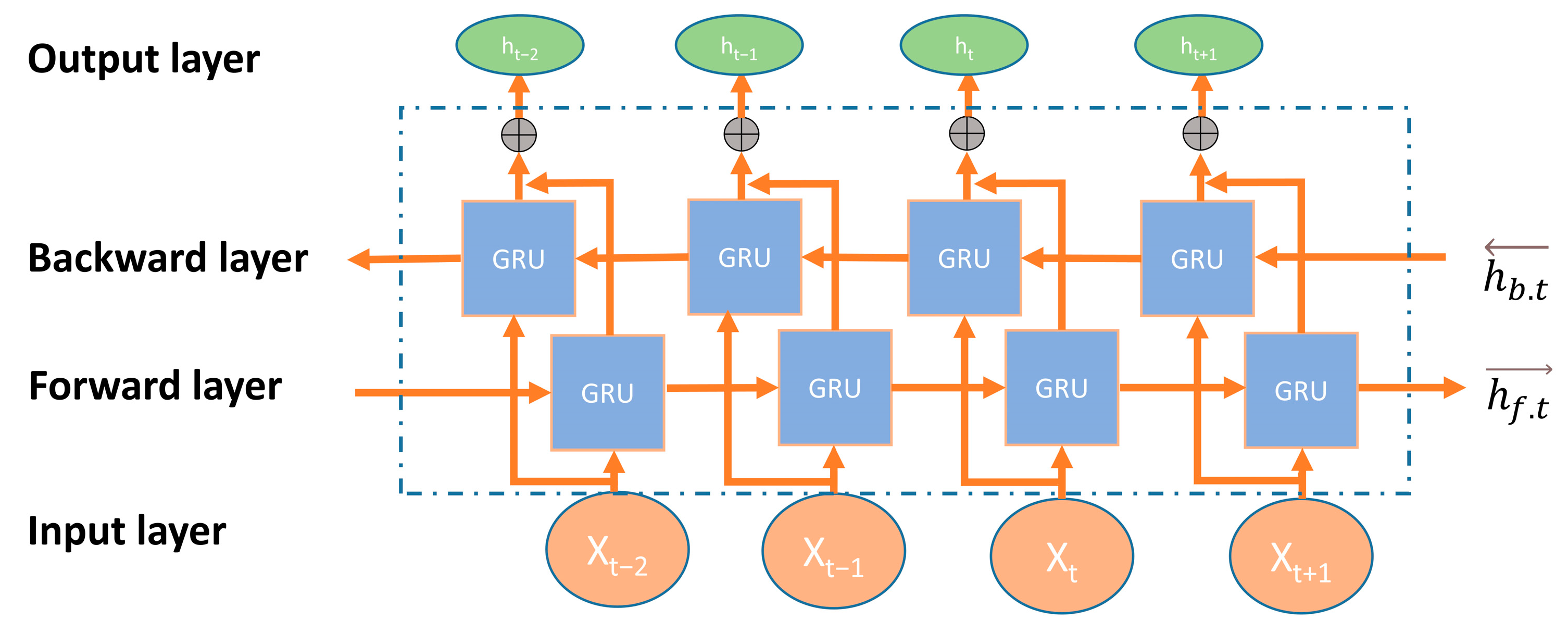
Pump station data, such as water level and flow, are correlated with each other before and after time t, not only depending on the information before time t, but also related to the information after time t. Therefore, Bi-GRU with bi-directional propagation structure can be selected to retain past and future information and combine the two kinds of information so that the model can better extract data features. Its structure is shown in Figure 4. It is composed of two one-way GRU structures in opposite directions. The first layer carries out unit coding from the forward direction and the second layer carries out unit coding from the reverse direction. The final output is determined by the combination of the two directions. The specific calculation structure is as follows:
h f . t = G f . t x t , h t 1
h b . t = G b . t x t , h t 1
h t = h f . t h b . t
where h f . t is in the positive state of GRU, h b . t is the GRU reverse state, G (.) represents the nonlinear transformation of the input data, represents the combination of h f . t and h b . t , h t is the hidden layer status at the current time.

2.5. Self-Attention Mechanism

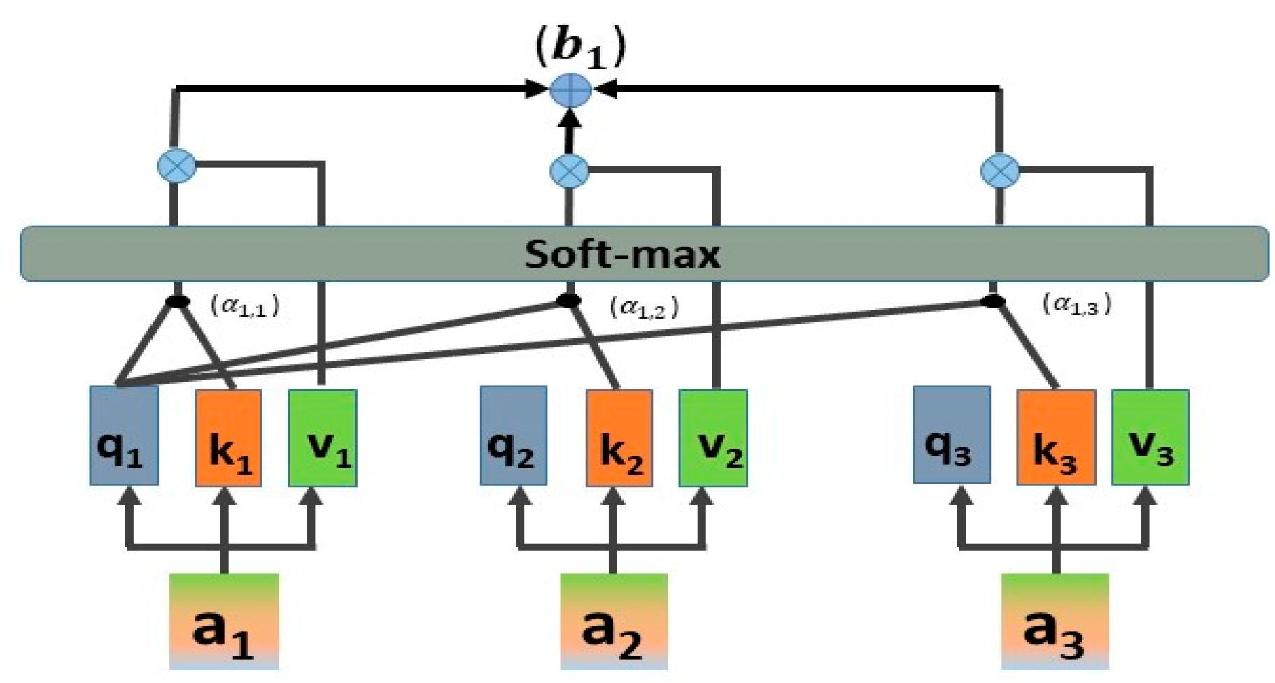
Similar to human visual cognition, attention mechanism focuses limited attention resources on key information, reduces attention to non-key information, and even ignores irrelevant information to achieve the goal of information screening. The application of attention mechanism to neural networks can enhance the information representation of key features. Attention mechanism has been widely used in machine learning. Self-attention mechanisms can establish long-distance dependencies within a sequence, regardless of the distance between elements within the sequence. The self-attention mechanism can be described as the mapping of a query to a series of key-value pairs. The calculation formula is as follows, and the working principle is shown in Figure 5.
A t t e n t i o n Q , K , V = S o f t m a x Q K T d V
The specific steps are as follows: (1) the input vector A , Q = W q . A , K = W k . A , V = W v . A , W q , W k , W v are the corresponding weights; (2) calculate the value of attention α , Q and K are used to calculate the correlation between each two input vectors, perform softmax operation on the matrix formed by α to obtain α , i , j , recorded as S o f t m a x ( . / d k ) ; (3) the input vector A corresponds to the output vector B; b i = j = 1 n v i . α , i , j , is the weighted sum of each value vector.
BiGRU has the problem of remote information loss when processing long time series. By adding a self-attention mechanism, it can calculate the weight of each feature in the hidden layer and output the feature information according to the weight, so that the network can better learn the information in the sequence and reduce the complexity of calculation. The BiGRU structure based on the self-attention mechanism is shown in Figure 6.

2.6. Autoregressive Integrated Moving Average Model

ARIMA model is one of the time series prediction models, which can reduce the in-fluence of interference items on the model. It is used to deal with non-stationary time se-ries, transform the original non-stationary series into stationary series through difference operation and then make modeling prediction. The model contains three parameters p, d, and q, denoted as ARIMA (p, q, d). Essentially, it is the combination of AR (p) model, MA(q) model and differential operation of sequence [41]. The model equation can be expressed as:
Δ d y t = μ + i = 1 p ϕ i Δ d y t i + ε t + i = 1 q θ j Δ d ε t j
p is the number of autoregressive terms; q is the number of moving average terms; d is the number of differences made for a sequence; ϕ i is the autocorrelation coefficient; θ j is the partial correlation coefficient; Δ d y t is a stationary time order after the d-order difference.
The steps for ARIMA modeling are as follows:
Step 1: the stationarity judgment. The unit root test (ADF) method is used to check whether the statistic P was less than 0.05 for the input sequence. If the data are stationary, the second step is carried out; otherwise, the d-order difference operation is performed to convert them to a stationary sequence.
Step 2: model order (p, d, q). The values of p and q are determined by the truncated and trailed graphs of autocorrelation coefficient (ACF) and partial correlation coefficient (PACF). For details, refer to Table 2.
In addition, in order to enhance the prediction ability of the model, Bayesian information criterion (BIC) is used to fit the model and further determine the optimal parameters. BIC considers the number of observations and has a greater penalty than the minimum information criterion (AIC) [42]. The BIC criteria are defined as follows:
B I C = K I n n 2 I n L
where k is the number of model parameters, n is the number of samples, and L is the likelihood function. The smaller the BIC value, the better the parameter.
Step 3: parameter test. By fitting the original data and adjusting the parameters to get the optimal regression coefficient, the accuracy of the model is improved.
Step 4: model test. Only by passing the white noise test can it be considered that the information extraction of the sequence can be fully analyzed and predicted; otherwise, return to step 1.
Step 5: model prediction.

2.7. Overall Framework

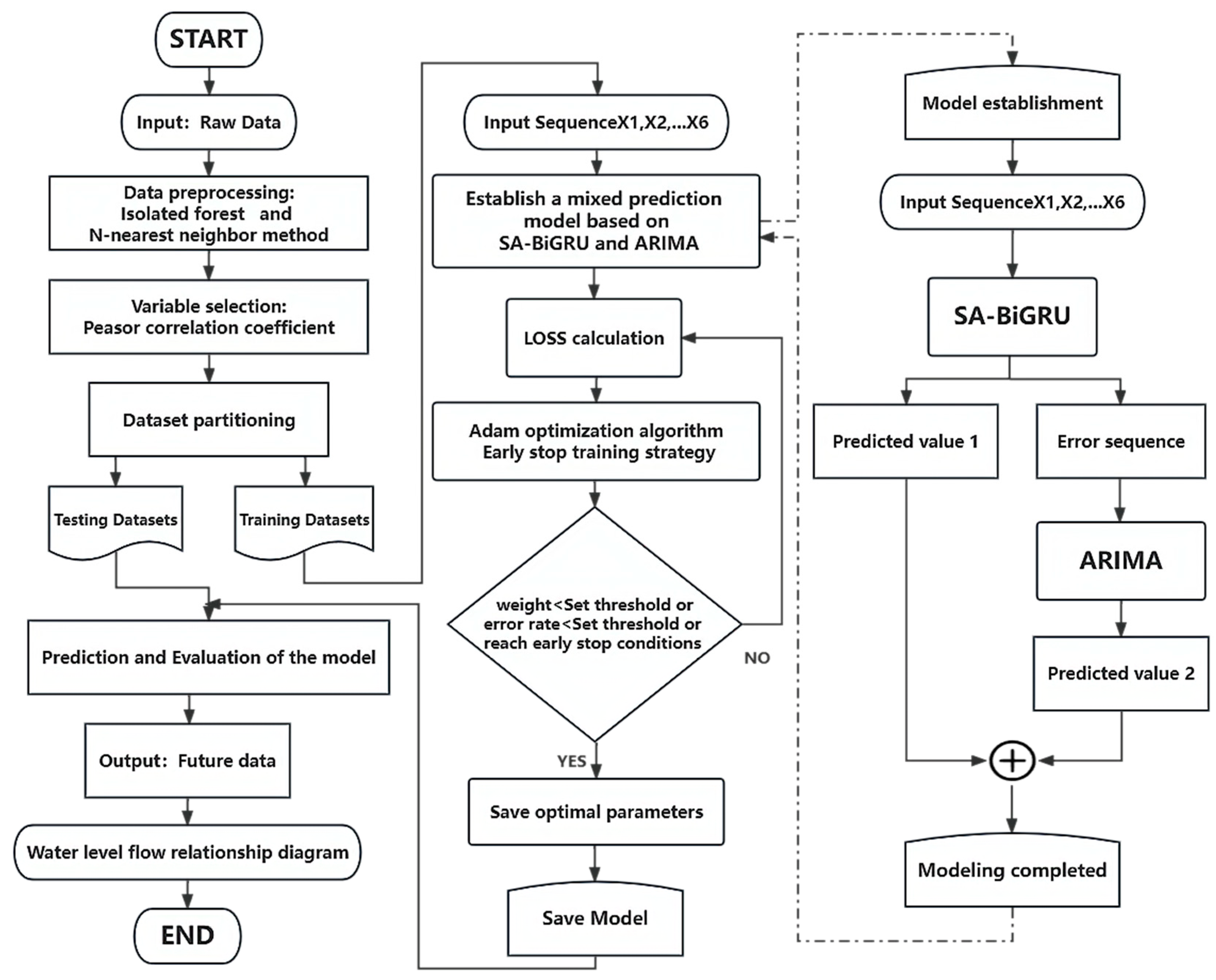
In this paper, combined with the BiGRU and ARIMA models introduced by the self-attention mechanism, a prediction model of the pumping station overflow capacity is constructed. The model is mainly divided into three parts. First, the pre-processing and feature selection of the timing sequence input are based on the attention mechanism BiGRU model, and the nonlinear features of the data are modeled. The BiGRU module is used to automatically extract the sequential features from the forward and reverse, and each feature is assigned a weight through the self-attention layer. Adam optimization algorithm is adopted to iteratively update the weight parameters of the network according to the trained data, and finally determine the optimal parameters of the BiGRU model and obtain the predicted values of the overflow and water level data, M1 and M2. Then, the error between the predicted value and the real value is calculated and the corresponding error sequences e1 and e2 are obtained. The second step uses the ARIMA model to extract the linear components of the residual sequence to correct the result value of the first step (that is, to generate the final error sequence E1 and E2), then the final predicted value Q = M + E. The third step is to draw a flow-level graph for further analysis of the overflow capacity.
The overall algorithm flow of the SA–BiGRU–ARIMA hybrid prediction model proposed in this paper is as follows:
  • The pumping station data is obtained, and the outliers in the data are processed by screening method, isolated forest algorithm and N-nearest neighbor algorithm. Then, Pearson correlation coefficient is used for feature selection and 6 variables with high correlation are selected as input variables. The pump station data from January to November 2020 are used as the training set, and the data from December as the test set.
  • Input variables into the SA–BiGRU model, and the feature sequences are reordered according to the weights obtained by the self-attention mechanism. Adam optimization algorithm and early-stop training strategy are used to select the optimal parameters, and the preliminary predicted value M is outputed by the full connection layer.
  • The error sequence obtained by SA–BiGRU is taken as the input vector of ARIMA model, and the prediction variable E of linear component of the error sequence is output after the stationarity test, model order determination and model fitting.
  • The final prediction variable Q = M + E is obtained by adding the prediction variables obtained in the second and third steps.
  • Finally, the test and evaluation are carried out, and the loss value is obtained according to the comparison between the output probability of the sample and the real value. The water-flow prediction relationship curve is then made.
The specific algorithm flow chart is shown in Figure 7.

2.8. Model Training and Evaluation

2.8.1. Training Strategy

Avoiding overfitting and underfitting of neural networks during training is a key problem in deep learning. Common approaches include using exit policies and regularization policies and configuring epochs appropriately [43]. All of these strategies need to be set before model training, so they cannot adapt well to the differences between different data sets and the randomness of the training process. The early-stop training strategy is an adaptive training strategy. It is possible to set the total period of model training to a larger value (such as 10,000) and determine whether to terminate the model training by monitoring the impact of the model on the validation data set. When the influence of the model on the validation data set is no longer improved in the time period, the model training is terminated and the optimal neural network parameters before the training termination are saved [44]. Therefore, the early-stop training strategy is selected in this paper.

2.8.2. Model Evaluation Index

To measure the prediction accuracy of the model, MAE, MAPE and R 2 are selected as the evaluation indexes. The calculation formula is as follows. Under the premise of predicting the same parameter, the smaller MAE and MAPE values, the more accurate the prediction results. R 2 represents the goodness of fit between the predicted value and the actual value; the closer it is to 1, the better the fitting effect of the data.
M A E = 1 n i = 1 n y i ^ y i
M A P E = 1 n i = 1 n y i ^ y i y i × 100 %
R 2 = 1 i = 1 n y i ^ y i 2 i = 1 n y i y 2
n is the total number of predictions; y i ^ represents the predicted value; y i represents the true value; y represents the mean.

3. Results and Discussion

3.1. Experimental Part

3.1.1. Data Processing and Experimental Environment

First, we used a screening method and isolated forest algorithm to process repeated values, outliers and missing values in the data. The proportion of outliers in the data is shown in Table 3. Then, N proximity algorithm was used to fill in the abnormal data.
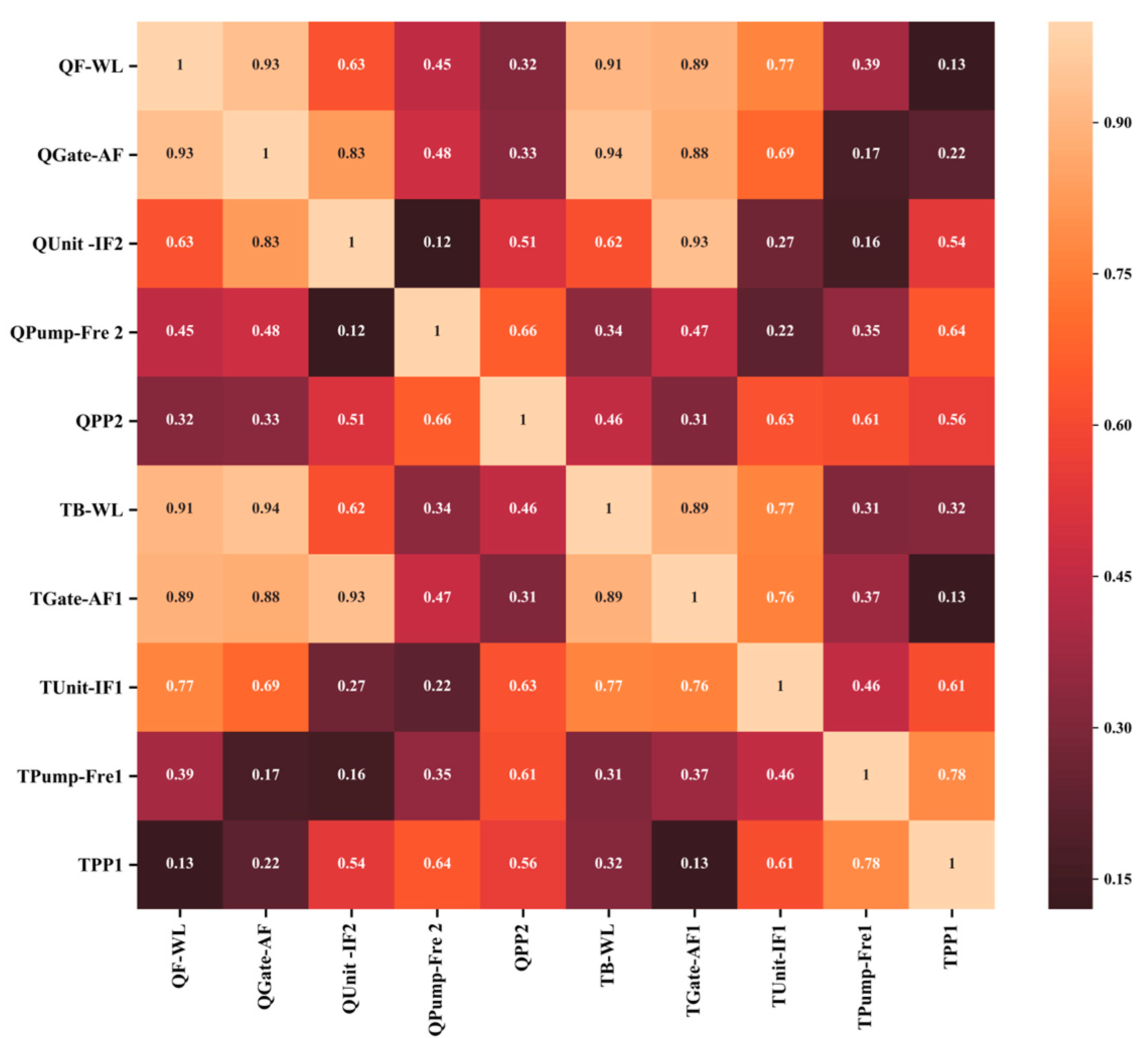
Overflow is not only related to water level and flow, but also affected by a variety of factors such as pump frequency, pipeline pressure and instantaneous flow of unit. However, each factor has a different degree of influence on overflow capacity. If each factor is unconditionally used as input for model prediction training, it will cause excessive model parameters and complicate the calculation process. Moreover, the factors with low correlation will interfere with the noise of the prediction results and reduce the prediction accuracy of the model. Through the Pearson correlation analysis of the pumping station data, only the influential factors with high correlation are screened out, and the thermal map results are shown in Figure 8. It can be seen that the Pearson correlation coefficients between QF-WL, TB-WL, TGate-AF1, QUnit-IF2 and TUnit-IF1 and over-traffic (QGate-AF) are all greater than 0.5. Therefore, QF-WL, TB-WL, TGate-AF1, QGate-AF, QUnit-IF2 and TUnit-IF1 with high Person correlation coefficient are finally selected as the final input variables of the model in this paper.
The data of the previous 1 to 11 months were selected as the training set, and the data of December were selected as the test set. The data acquisition interval adopted in this paper is 1 min. Because water level, flow rate and other factors do not change significantly in a short time, the average value of 30 sampling points is used to replace the original 30 sampling points, making the time interval of sample points become 30 min. In this way, the model can realize the prediction of data after 30 min.
The environment used in the experiment was Window10 operating system, the processor was AMD A10-8700P Radeon R6, the CPU frequency was 1.8 GHZ, and the memory was 8 GB. The programming language is Python3.7, and Keras under the framework of Tensorflow2.0 is used to implement it.

3.1.2. Model Parameter Setting

In the process of BiGRU model training, the correct selection of hyper-parameters is very important to improve the model performance. In this paper, the batch size was 240, and the weight of the model was updated iteratively for 10 rounds. The hidden layer was set as 2, which were the forward and reverse propagation layers of the BiGRU model, and the number of neurons was set as 64 and 128, respectively. The Adam optimizer was used. The learning rate adopted exponential decay formula, the initial value was 0.01 and the fading factor was 0.8. The training error was set to 0.0001. The dropout layer was added to the BiGRU network to avoid overfitting the model, and the dropout size was set to 0.5. In addition, the adaptive early-stop training strategy was added to further select the optimal parameters, and the maximum training period was set to 2000.
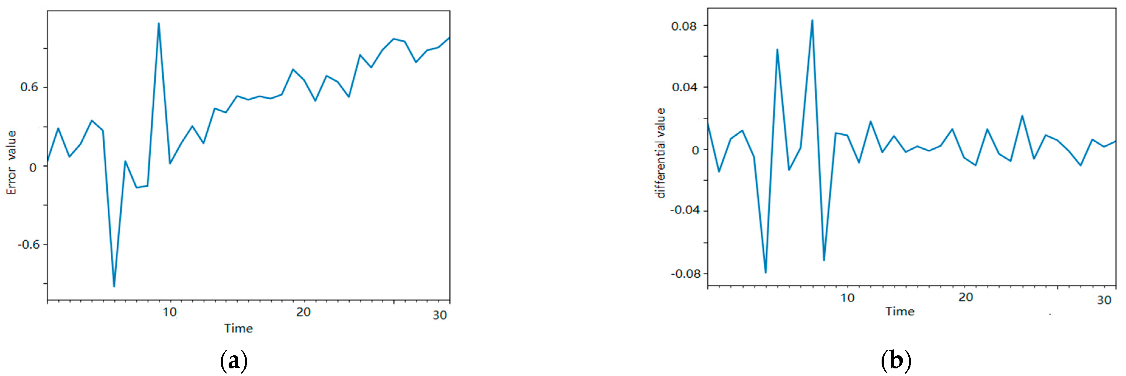
ARIMA (p, d, q) was determined. Firstly, it can be seen from Figure 9a that the error sequence of overflow (QGate-AF) has a monotonically increasing trend and is preliminarily judged to be a non-stationary sequence. After an ADF test, P = 0.887 > 0.05, d-order difference calculation is carried out. The result of the error sequence after first-order difference is shown in Figure 9b. The ADF unit root test is conducted again on the sequence after first-order difference, and the test result P = 0.003 < 0.05 rejects the original hypothesis, and then the time series after first-order difference is stable, i.e., d = 1. The water level (QF-WL) error sequence d = 0 can be obtained by using the same method.
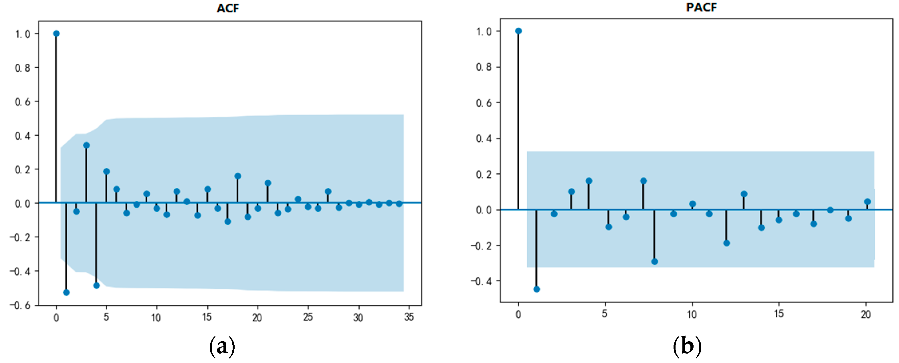
Secondly, ACF diagrams and PACF diagrams were made through the sequence after difference, as shown in Figure 10. Truncated ACF and PACF appear after the first order respectively, and the values of p and q are preliminarily determined to be 1, 1 respectively. Then, the BIC criterion is used to verify that (1, 1) are the optimal values of p and q, respectively. Similarly, the optimal p and q of the water level error sequence are (0, 1).
From Figure 9, it can be seen that the sequence after difference does not have obvious time periodicity, and combined with Figure 10, the ACF and PACF function plots show good trailing or truncation, so it can be considered as less influenced by seasonal factors.

3.2. Result Analysis

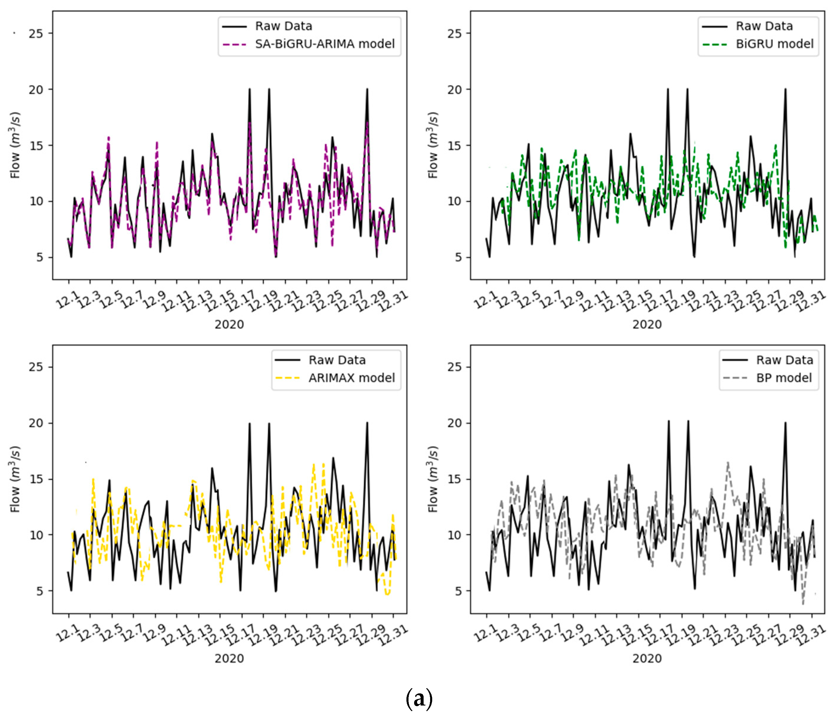
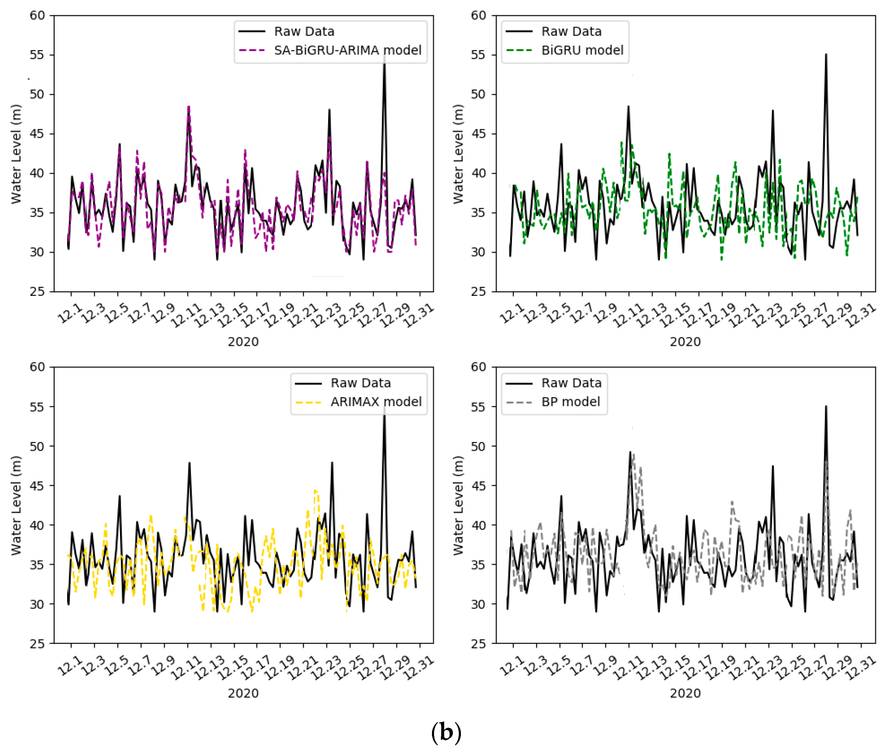
In order to verify the effectiveness of the model selected in this study, ARIMAX, BiGRU and BP neural network all used the same parameter settings to predict the overflow and water level of the pumping station in December 2020. The final prediction results are shown in Figure 11.
As can be seen from Figure 11, the SA–BiGRU–ARIMA, BiGRU, ARIMAX and BP neural network models can roughly capture the changing trends of flow and water level, among which the SA–BiGRU–ARIMA model can accurately identify the changes of peak value brought by extreme weather or human factors. It can fit the whole fluctuation well. However, there is also a certain amount of prediction error, including changes caused by special factors, such as unit power outage and pump station failure, which cannot be effectively addressed. For the prediction of overflow, the BiGRU model can also roughly capture the trend of overflow changes, but it cannot fit well in extreme situations and may result in high predicted values. For the traditional machine learning model ARIMAX, although it can predict multivariate time series, it is not sensitive to nonlinear components in the sequence, resulting in significant errors. For BP neural networks, significant errors also occur due to the strong dependence on initialization weights and biases. In order to comprehensively verify the prediction effect of the four groups of experiments, MAE, MAPE and R2 were used as evaluation indexes. The evaluation results are shown in Table 4.
Compared with the single BiGRU, ARIMAX and BP neural network models, MAE, MAPE and R2 of the hybrid SA–BiGRU–ARIMA model were significantly improved. In terms of data fitting, for the overflow prediction, compared to the BiGRU model alone, ARIMAX model, and BP neural network model, the MAE decreased by 6.55%, 11.13% and 9.05%, respectively, indicating that the selected model in this paper has the lowest overall deviation from the actual data and the stability of the fit is higher, with the BiGRU model being the second most stable; compared with the BiGRU model alone, ARIMAX model, and BP neural network model, MAPE decreased by 1.59%, 8.08% and 3.24%, respectively, and the model selected in this paper has the lowest MAPE value, indicating a better fit; the R2 value of the model selected in this paper is 0.87, the R2 value of the BiGRU model is 0.61, the R2 value of the ARIMAX model is 0.37 and the R2 value of the BP model is 0.42. The model selected in this paper has the highest R2 value, and in a comprehensive view the SA–BiGRU–ARIMA model has a higher fitting accuracy in the prediction of the overflow. For the water level prediction, compared with the BiGRU model, ARIMAX model, and BP neural network model alone, the MAE decreased by 10.75%, 38.53% and 15.87%, respectively, indicating that the model selected in this paper has the lowest overall deviation from the actual data, and the stability of the fit is higher, and the BiGRU model model is the second most stable; compared with the BiGRU model, ARIMAX model and BP neural network model alone, the MAPE is reduced by 3.61%, 12.05% and 10.12%, respectively, and the model selected in this paper has the lowest MAPE value, indicating a better fit; the selected model in this paper has an R2 value of 0.81, the BiGRU model has an R2 value of 0.56, the ARIMAX model has an R2 value of 0.43 and the BP model has an R2 value of 0.44. The selected model in this paper has the highest R2 values, which are improved by 0.25, 0.38 and 0.37, respectively. Collectively, the SA–BiGRU–ARIMA model has the highest R2 value for water level prediction with high fitting accuracy.
In terms of data prediction, comparing the MAE values, the SA–BiGRU–ARIMA model has the smallest MAE value among the four models, indicating that the predicted value is closer to the true value. Comparing the MAPE indicator values, the SA–BiGRU–ARIMA model has the smallest MAPE value among the four models, which meets the criteria of high precision prediction.
In summary, the SA–BiGRU–ARIMA model takes into account several factors affecting the overflow, and the three evaluation indexes of MAE value, MAPE index value and R2 value are optimal in overflow and water level prediction and data fitting. This indicates that the model has good applicability for the simulation and prediction of the overflow of the former Liulin pumping station, and can better respond to the fluctuating trend of overflow, with high and robust prediction accuracy.
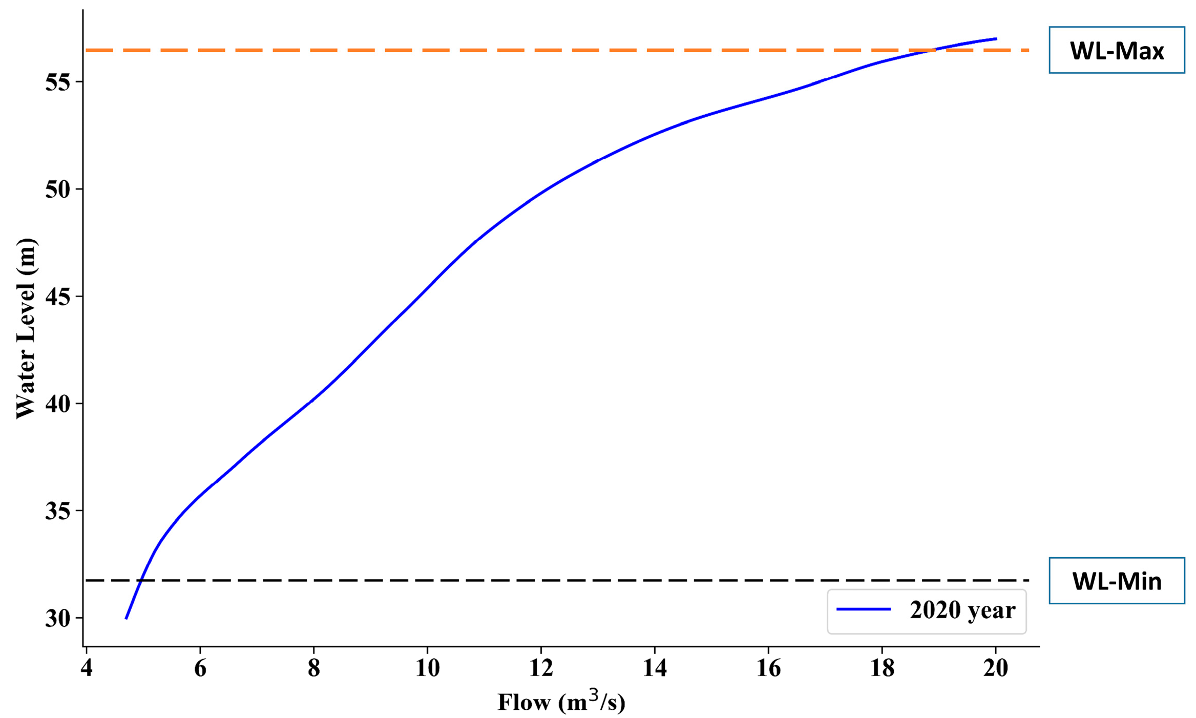
Figure 12 shows the relation curve between water level and flow of QianLiulin Pump Station before 2020. Generally, there is a positive correlation between the flow capacity of the pumping station and the water level. If the maximum warning water level is set to 50 m, the reference flow range is 12–14 m3/s. If the maximum flow is set to 15 m3/s, the water level control range can be set to less than 52 m. Therefore, flood control measures can be taken in advance through the relationship between discharge and water level. The flow-water level can be adjusted according to demand. The specific overflow capacities at different water levels are shown in Table 5.

4. Conclusions

In this paper, an SA–BiGRU–ARIMA overflow capacity prediction model is established on the basis of considering the influence of factors such as water level and discharge. It not only solves the problems of complex physical and mathematical modeling structure and time-consuming calculation, but also improves the effect of single neural network model on the prediction of overflow capacity. Firstly, query method, isolated forest method and N-nearest neighbor algorithm are used to process outliers in the data, and Pearson correlation coefficient is used for feature selection. Then, by introducing the BiGRU model with self-attentional mechanism, we focus on learning the key features to better process the linear components of the data. We also add the double-layer dropout layer to avoid overfitting. Finally, the residual sequence was used to correct the nonlinear components of the data extracted by the ARIMA model, and the water-flow relationship diagram was drawn according to the predicted results for specific analysis. Compared with the BiGRU model, ARIMAX model and BP neural network model, the SA–BiGRU–ARIMA model performs better in data fitting and prediction; the indicators are optimal, indicating that the model has better applicability for the prediction of overflow; the calculation accuracy is high; and the model is robust, which can provide technical guidance and theoretical reference for flood control dispatching and water demand in the actual pump station construction project.
Although the model proposed in this paper shows good performance, the changes brought by some unusual factors, such as unit power failure, pump station failure and other special factors, may still cause large errors, resulting in unsatisfactory prediction results. In addition, the method is only applicable to the data of the pumping station of Miyun Reservoir regulation and storage project at present. In the future, the data of other pumping stations can be further used for training, so as to further enhance the universality and generalization of the model. Secondly, the unit operating parameters, the degree of water grass and sediment in the channel and the resistance of the river channel can also be considered to further improve the accuracy of the model.

Author Contributions

Conceptualization, J.Y.; Methodology, T.G. and J.Y.; software, T.G.; validation, Y.Y. and T.G.; formal analysis, J.Y.; investigation, T.G.; resources, J.Y.; writing—original draft, T.G.; writing—review and editing, T.G. supervision, J.Y., T.G., Y.Y. and J.C. All authors have read and agreed to the published version of the manuscript.

Funding

This research received no external funding.

Data Availability Statement

The data in this study can be obtained by contacting the author’s email.

Conflicts of Interest

The authors declare no conflict of interest.

References

  1. Lee, E.; Kim, J. Convertible Operation Techniques for Pump Stations Sharing Centralized Reservoirs for Improving Resilience in Urban Drainage Systems. Water 2017, 9, 843. [Google Scholar] [CrossRef] [Green Version]
  2. Wang, J.; Chang, T.; Chen, J. An enhanced genetic algorithm for bi-objective pump scheduling in water supply. Expert Syst. Appl. 2009, 36, 10249–10258. [Google Scholar] [CrossRef]
  3. Slater, L.J. To what extent have changes in channel capacity contributed to flood hazard trends in England and Wales? Earth Surf. Process. Landf. 2016, 41, 1115–1128. [Google Scholar] [CrossRef] [Green Version]
  4. Naito, K.; Parker, G. Can Bankfull Discharge and Bankfull Channel Characteristics of an Alluvial Meandering River be Cospecified from a Flow Duration Curve? J. Geophys. Res. Earth Surf. 2019, 124, 2381–2401. [Google Scholar] [CrossRef]
  5. Suzhen, H.; Ping, W.; Yan, G.; Ting, L. Response of bankfull discharge of the Inner Mongolia Yellow River to flow and sediment factors. J. Earth Syst. Sci. 2014, 123, 1307–1316. [Google Scholar]
  6. Hermann, M.F.; Willi, H.H. Hydraulics of Embankment Weirs. J. Hydraul. Eng. ASCE 1998, 124, 963–971. [Google Scholar]
  7. Yang, K.; Liu, X.; Cao, S.; Huang, E. Stage-Discharge Prediction in Compound Channels. J. Hydraul. Eng. ASCE 2014, 140, 06014001. [Google Scholar] [CrossRef]
  8. Chen, G.; Zhao, S.; Huai, W.; Gu, S. General model for stage-discharge prediction in multi-stage compound channels. J. Hydraul. Res. 2019, 57, 517–533. [Google Scholar] [CrossRef]
  9. Zheng, H.; Lei, X.; Shang, Y.; Cai, S.; Kong, L.; Wang, H. Parameter identification for discharge formulas of radial gates based on measured data. Flow Meas. Instrum. 2017, 58, 62–73. [Google Scholar] [CrossRef]
  10. Bijankhan, M.; Mazdeh, A.M. Assessing Malcherek’s Outflow Theory to Deduce the Theoretical Stage-Discharge Formula for Overflow Structures. J. Irrig. Drain. Eng. ASCE 2018, 144, 6018007. [Google Scholar] [CrossRef]
  11. Fencl, M.; Grum, M.; Borup, M.; Mikkelsen, P.S. Robust model for estimating pumping station characteristics and sewer flows from standard pumping station data. Water Sci. Technol. 2019, 79, 1739–1745. [Google Scholar] [CrossRef] [PubMed]
  12. Timbadiya, P.V.; Patel, P.L.; Porey, P.D. A 1D-2D Coupled Hydrodynamic Model for River Flood Prediction in a Coastal Urban Floodplain. J. Hydrol. Eng. 2015, 20, 5014017. [Google Scholar] [CrossRef]
  13. Karim, F.; Marvanek, S.; Wallace, J. The use of hydrodynamic modelling and remote sensing to assess hydrological connectivity of floodplain wetlands. In Hydrology and Water Resources Symposium; Engineers Australia: Barton, ACT, Australia, 2012; pp. 1334–1341. [Google Scholar]
  14. Lv, Y.; Chi, R. Data-driven adaptive iterative learning predictive control. In Proceedings of the 2017 6th Data Driven Control and Learning Systems (DDCLS), Chongqing, China, 26–27 May 2017. [Google Scholar]
  15. Contreras, J.; Espinola, R.; Nogales, F.J.; Conejo, A.J. ARIMA models to predict next-day electricity prices. IEEE Trans. Power Syst. 2003, 18, 1014–1020. [Google Scholar] [CrossRef]
  16. Noori, R.; Karbassi, A.R.; Moghaddamnia, A.; Han, D.; Zokaei-Ashtiani, M.H.; Farokhnia, A.; Gousheh, M.G. Assessment of input variables determination on the SVM model performance using PCA, Gamma test, and forward selection techniques for monthly stream flow prediction. J. Hydrol. 2011, 401, 177–189. [Google Scholar] [CrossRef]
  17. Wang, X.; Liu, T.; Zheng, X.; Peng, H.; Xin, J.; Zhang, B. Short-term prediction of groundwater level using improved random forest regression with a combination of random features. Appl. Water Sci. 2018, 8, 125. [Google Scholar] [CrossRef] [Green Version]
  18. Kisi, O.; Kerem Cigizoglu, H. Comparison of different ANN techniques in river flow prediction. Civ. Eng. Environ. Syst. 2007, 24, 211–231. [Google Scholar] [CrossRef]
  19. Schuster, M.; Paliwal, K.K. Bidirectional recurrent neural networks. IEEE Trans. Signal Process. 1997, 45, 2673–2681. [Google Scholar] [CrossRef] [Green Version]
  20. Yan, G.; Ping, W.; Suzhen, H.; Huan, W. Prediction of flow capacity of the Inner Mongolia section of the Yellow River based on BP neural network. J. Water Resour. Constr. Eng. 2021, 19, 246–251. (In Chinese) [Google Scholar]
  21. Qiu, Y.; Yang, Z.; Zhou, Y.; Wu, J.; Xie, H. Prediction of Flow Capacity of Right Angle Broken Line Weir Based on BP Neural Network. Hydroelectr. Energy Sci. 2021, 39, 74–77. (In Chinese) [Google Scholar]
  22. Wei, C.; Hsu, N.; Huang, C. Two-Stage Pumping Control Model for Flood Mitigation in Inundated Urban Drainage Basins. Water Resour. Manag. 2014, 28, 425–444. [Google Scholar] [CrossRef]
  23. Ghorbani, M.A.; Deo, R.C.; Kim, S.; Hasanpour Kashani, M.; Karimi, V.; Izadkhah, M. Development and evaluation of the cascade correlation neural network and the random forest models for river stage and river flow prediction in Australia. Soft Comput. 2020, 24, 12079–12090. [Google Scholar] [CrossRef]
  24. Elbeltagi, A.; Di Nunno, F.; Kushwaha, N.L.; de Marinis, G.; Granata, F. River flow rate prediction in the Des Moines watershed (Iowa, USA): A machine learning approach. Stoch. Environ. Res. Risk Assess. 2022, 11, 3835–3855. [Google Scholar] [CrossRef]
  25. Darwen, P.J. Bayesian model averaging for river flow prediction. Appl. Intell. 2019, 49, 103–111. [Google Scholar] [CrossRef]
  26. Tan, P.C.; Berger, C.S.; Dabke, K.P.; Mein, R.G. Recursive identification and adaptive prediction of wastewater flows. Automatica 1991, 27, 761–768. [Google Scholar] [CrossRef]
  27. Musarat, M.A.; Alaloul, W.S.; Rabbani, M.B.A.; Ali, M.; Altaf, M.; Fediuk, R.; Vatin, N.; Klyuev, S.; Bukhari, H.; Sadiq, A.; et al. Kabul River Flow Prediction Using Automated ARIMA Forecasting: A Machine Learning Approach. Sustainability 2021, 13, 10720. [Google Scholar] [CrossRef]
  28. Pierini, J.O.; Gomez, E.A.; Telesca, L. Prediction of water flows in Colorado River, Argentina. Lat. Am. J. Aquat. Res. 2012, 40, 872–880. [Google Scholar] [CrossRef]
  29. Xu, W.; Jiang, Y.; Zhang, X.; Li, Y.; Zhang, R.; Fu, G. Using long short-term memory networks for river flow prediction. Hydrol. Res. 2020, 51, 1358–1376. [Google Scholar] [CrossRef]
  30. Aryal, S.K.; Zhang, Y.; Chiew, F. Enhanced low flow prediction for water and environmental management. J. Hydrol. 2020, 584, 124658. [Google Scholar] [CrossRef]
  31. Li, Y.; Zhu, Z.; Kong, D.; Han, H.; Zhao, Y. EA-LSTM: Evolutionary attention-based LSTM for time series prediction. Knowl. Based Syst. 2019, 181, 104785. [Google Scholar] [CrossRef] [Green Version]
  32. Li, X.; Xu, W.; Ren, M.; Jiang, Y.; Fu, G. Hybrid CNN-LSTM models for river flow prediction. Water Supply 2022, 22, 4902–4919. [Google Scholar] [CrossRef]
  33. Zhang, X.; Qiao, W.; Huang, J.; Shi, J.; Zhang, M. Flow prediction in the lower Yellow River based on CEEMDAN-BILSTM coupled model. Water Supply 2023, 23, 396–409. [Google Scholar] [CrossRef]
  34. Lv, N.; Liang, X.; Chen, C.; Zhou, Y.; Li, J.; Wei, H.; Wang, H. A long Short-Term memory cyclic model with mutual information for hydrology forecasting: A Case study in the xixian basin. Adv. Water Resour. 2020, 141, 103622. [Google Scholar] [CrossRef]
  35. Chen, C.; Luan, D.; Zhao, S.; Liao, Z.; Zhou, Y.; Jiang, J.; Pei, Q. Flood Discharge Prediction Based on Remote-Sensed Spatiotemporal Features Fusion and Graph Attention. Remote Sens. 2021, 13, 5023. [Google Scholar] [CrossRef]
  36. Wu, B.; Wang, G.; Xia, J.; Fu, X.; Zhang, Y. Response of bankfull discharge to discharge and sediment load in the Lower Yellow River. Geomorphology 2008, 100, 366–376. [Google Scholar] [CrossRef]
  37. Tang, X. An improved method for predicting discharge of homogeneous compound channels based on energy concept. Flow Meas. Instrum. 2017, 57, 57–63. [Google Scholar] [CrossRef]
  38. Liu, F.T.; Ting, K.M.; Zhou, Z.H. Isolation-based anomaly detection. ACM Trans. Knowl. Discov. Data TKDD 2012, 6, 1–39. [Google Scholar] [CrossRef]
  39. Zhang, Y.; Dai, H.; Xu, C.; Feng, J.; Wang, T.; Bian, J.; Wang, B.; Liu, T.Y. Sequential Click Prediction for Sponsored Search with Recurrent Neural Networks. In Proceedings of the AAAI Conference on Artificial Intelligence, Quebec City, QC, Canada, 27–31 July 2014. [Google Scholar]
  40. Dey, R.; Salem, F.M. Gate-variants of gated recurrent unit (GRU) neural networks. In Proceedings of the 2017 IEEE 60th International Midwest Symposium on Circuits and Systems (MWSCAS), Boston, MA, USA, 6–9 August 2017. [Google Scholar]
  41. Mauludiyanto, A.; Hendrantoro, G.; Purnomo, M.H.; Ramadhany, T.; Matsushima, A. ARIMA Modeling of Tropical Rain Attenuation on a Short 28-GHz Terrestrial Link. IEEE Antennas Wirel. Propag. Lett. 2010, 9, 223–227. [Google Scholar] [CrossRef]
  42. Vrieze, S.I. Model selection and psychological theory: A discussion of the differences between the Akaike information criterion (AIC) and the Bayesian information criterion (BIC). Psychol. Methods 2012, 17, 228–243. [Google Scholar] [CrossRef] [Green Version]
  43. Dahl, G.E.; Sainath, T.N.; Hinton, G.E. Improving deep neural networks for LVCSR using rectified linear units and dropout. In Proceedings of the 2013 IEEE International Conference on Acoustics, Speech and Signal Processing, Vancouver, BC, Canada, 26–31 May 2013. [Google Scholar]
  44. Chen, L.; Yan, H.; Yan, J.; Wang, J.; Tao, T.; Xin, K.; Li, S.; Pu, Z.; Qiu, J. Short-term water demand forecast based on automatic feature extraction by one-dimensional convolution. J. Hydrol. 2022, 606, 127440. [Google Scholar] [CrossRef]
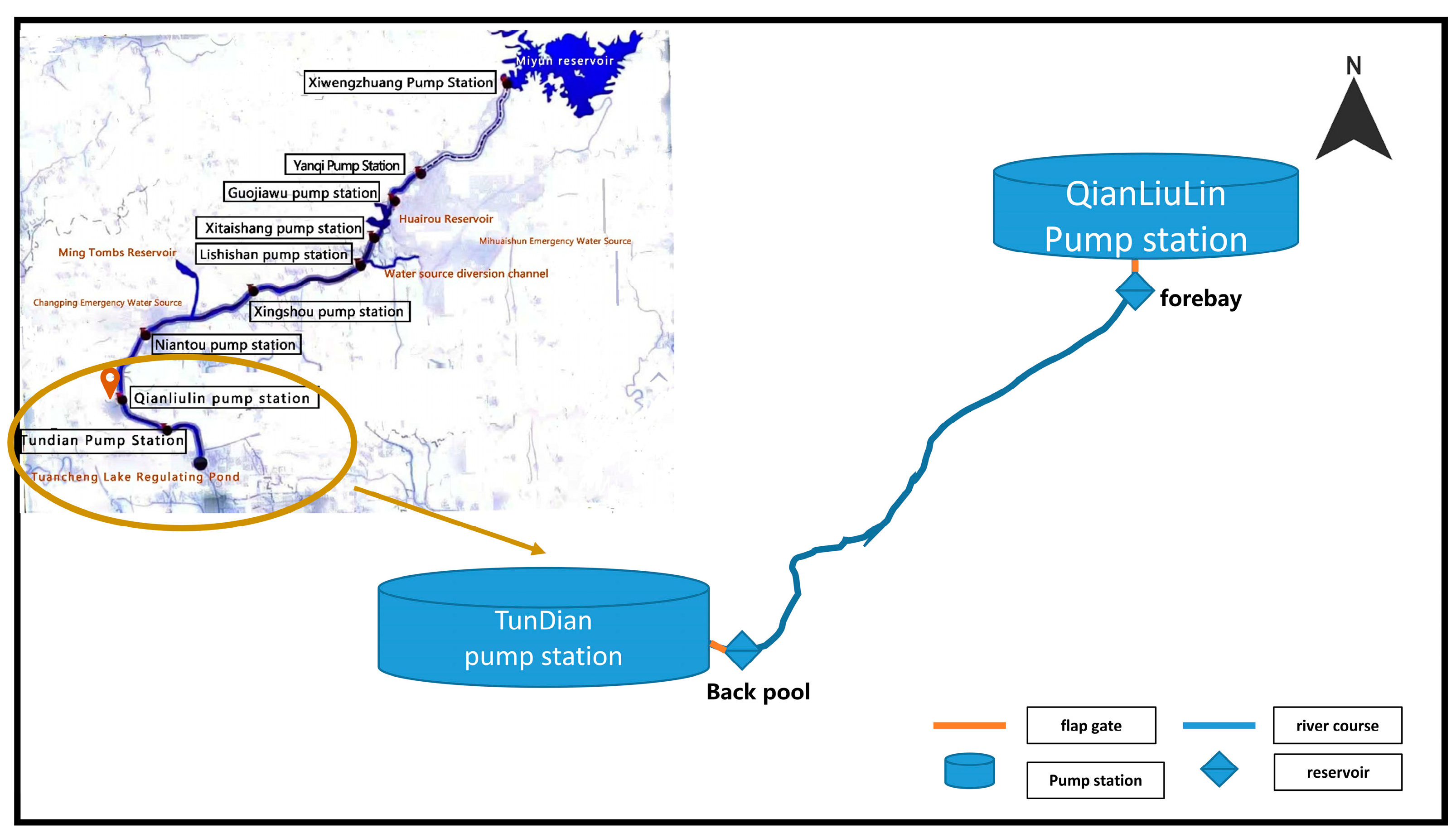
Figure 1. Study area map.
Water 15 02380 g001
Figure 2. Flow chart of the isolated forest algorithm.
Water 15 02380 g002
Figure 3. (a) RNN structure diagram; (b) GRU structure diagram.
Water 15 02380 g003
Figure 4. Bi-GRU structure diagram.
Water 15 02380 g004
Figure 5. Structure diagram of self-attention mechanism.
Water 15 02380 g005
Figure 6. BiGRU-attention model structure.
Water 15 02380 g006
Figure 7. Overall algorithm flow chart.
Water 15 02380 g007
Figure 8. Heat maps of Pearson correlation coefficients.
Water 15 02380 g008
Figure 9. (a) Residual sequence; (b) Sequence after difference.
Water 15 02380 g009
Figure 10. (a) ACF diagram; (b) PACF diagram.
Water 15 02380 g010
Figure 11. (a) Overflow prediction results; (b) water level prediction results.
Water 15 02380 g011aWater 15 02380 g011b
Figure 12. Changes of water-flow relationship.
Water 15 02380 g012
Table 1. The data information and statistical characteristics.
DataDescriptionMean ValueMaximum ValueMinimum ValueStandard DeviationUnit
TB-WLBack-pool water level40.3665.7523.2140.73m
TGate-AF1Gate accumulated flow111.28205.223.26m3/s
TUnit-IF1Unit instantaneous flow11.7421.431.57m3/s
TPump-Fre1pump frequency 137502518.32Hz
TPP1Pipeline pressure11.11.60.60.56Mpa
QF-WLForebay water level35.2558.3220.3442.56m
QGate-AFGate accumulated flow210.37204.716.71m3/s
QUnit-IF2Unit instantaneous flow21.681.991.450.98m3/s
QPump-Fre 2pump frequency 232502012.11Hz
QPP2Pipeline pressure21.21.60.70.33Mpa
Note(s): the English abbreviations of each data are used for the convenience of the subsequent use of the article to avoid repeated and lengthy information.
Table 2. Parameter identification table of ARIMA model (p,q).
FeaturesAR (p)MA (q)ARMA (p,q)
ACFtrailingqth order back truncationtrailing
PACFpth order back truncationfeaturestrailing
Note(s): ACF describes the correlation between the time-series data themselves; PACF describes the relationship between the values of the time series and their lags.
Table 3. Comparison of processing results of missing values.
Impact FactorsrQF-WLQGate-AFQUnit -IF2QPump-Fre 2QPP2TB-WLTGate-AF1TUnit-IF1TPump-Fre1TPP1
Outlie(%)1.31.12.92.82.21.72.32.13.02.3
Table 4. Comparison model evaluation indexes.
DataIndicatorModel
SA–BiGRU–ARIMABiGRUARIMAXBP
QGate-AFMAE9.3215.8720.4518.37
MAPE (100%)7.388.9715.4610.62
R20.870.610.370.42
QF-WLMAE18.7829.5357.3134.65
MAPE (100%)6.7310.3418.7816.85
R20.810.560.430.44
Table 5. The QianLiulin pumping station 2020 overflow capacity.
Water Level(m)Flow (m3/s)Water Level (m)Flow (m3/s)
408.04812.0
429.05013.0
4410.05214.0
4611.05415.0
Disclaimer/Publisher’s Note: The statements, opinions and data contained in all publications are solely those of the individual author(s) and contributor(s) and not of MDPI and/or the editor(s). MDPI and/or the editor(s) disclaim responsibility for any injury to people or property resulting from any ideas, methods, instructions or products referred to in the content.