A New Model for Solving Hydrological Connectivity Inside Soils by Fast Field Cycling NMR Relaxometry

Abstract

In this paper, a new quantitative approach for estimating the structural and functional connectivity inside soil by Fast Field Cycling (FFC) NMR relaxometry is presented, tested by measurements carried out in three samples with different texture characteristics. Measurements by FFC NMR relaxometry have been carried out using water-suspended samples and Proton Larmor frequencies (ν_L) ranging in the 0.015–35 MHz interval. Two non-degraded soil samples, with different textural characteristics, and a degraded soil collected in a badland area, were analyzed. For a given soil and any applied Proton Larmor frequency, the distribution of the longitudinal relaxation times, T₁, (i.e., relaxogram) measured by FFC NMR has been integrated, and the resulting S-shaped curve (i.e., relaxogram integration curve) was represented, for the first time, by Gumbel’s diagram. This new representation of the relaxogram integration curve, transforming the S-shaped curve into a straight line, allowed for distinguishing three linear components, corresponding to three different relaxation time ranges, characterized by three different slopes. Two points, identified by the abrupt slope changes of the relaxogram integration curve plotted in Gumbel’s diagram, are used to identify two characteristic values of relaxation time, T_1A and T_1B, which define three well-known pore size classes (T₁ < T_1A micro-pores, T_1A < T₁ < T_1B meso-pores, and T₁ > T_1B macro-pores). The relaxogram integration curve allowed for calculating the non-exceeding empirical cumulative frequency, F(T₁), corresponding to the characteristic T_1A and T_1B values. The analysis demonstrated that the relaxogram can be used to determine the pore-size ranges of each investigated sample. Finally, using the slope values of the three components of the relaxogram integration curve, a new definition of the Structural Connectivity Index, SCI, and Functional Connectivity Index, FCI, was proposed.

1. Introduction

The term “Connectivity” is used to express how an environmental system facilitates the matter and energy transfer within or among its elements (e.g., basin, soil) [1,2]. This concept was originally introduced in ecology [3] and was then widely used in other scientific fields (e.g., land systems, catchment hydrology, geomorphology, soil erosion, and sedimentation). For a given temporal and spatial scale [4], this concept allows for representing the capability of a vector, such as water, to transport materials [5,6], considering both the complexity and heterogeneity of a non-homogeneous environmental system. Despite the popularity of this concept among researchers, no shared definition and no common measurement technique of hydrological connectivity exist [7]. Wainwright et al. [8] suggested that each environmental system can be characterized by structural and functional connectivity. Structural connectivity is a property of the environmental system that expresses the contiguity of different features and the mutual physical connection [9,10]. For example, the water movement inside the soil is affected by its texture (associated with soil particle sizes) and structure (associated with the particle spatial arrangements). Consequently, soil texture and structure are information useful to determine soil structural connectivity and evaluate the effects on water infiltration inside the soil. The structural connectivity allows for representing how the interactions among structural characteristics of the investigated system affect the studied process [11].

Bracken and Crooke [12] refer to a catchment as a reference physical environment to distinguish three types of connectivity: landscape connectivity, hydrological connectivity, and sedimentological connectivity. For this investigated physical system, the terms landscape, hydrological, and sedimentological connectivity consider the connection among landscape units, the water movement through the system, and the sediment transport through the system elements, respectively [13].

For an investigated environmental system, functional connectivity expresses the effects of the interactions among the structural components on a specific process (ecological, hydrological, geomorphological) [8]. All things considered, structural connectivity gives a stationary (time-independent) point of view of the investigated system, while functional connectivity represents its dynamic response.

The concept of hydrological connectivity inside the soil (HCS) was introduced in previous studies [14,15,16,17] to represent how the interaction of soil spatial patterns (i.e., the structural connectivity SC) with physical and chemical processes (i.e., the functional connectivity FC) can affect the water transfer inside the soil. Furthermore, flow motion inside the soil (infiltration) influences the quote of rainfall generating surface runoff, which is also determining for sediment transport phenomena [14]. The structural component, SC, considers the spatial arrangement of soil particles which affects the organization of soil pores and channels. The functional component, FC, considers the water movement inside soil pores or aggregates and the effects of the chemical¬–physical interactions of water with the pore boundaries.

Conte and Ferro [15,16,17] demonstrated that nuclear magnetic resonance (NMR) relaxometry with the Fast Field Cycling (FFC) setup is useful to measure HCS and its components SC and FC. An overview about the possible applications of FFC NMR relaxometry is given in the paper by Conte [18]. This technique applies a fast change of the magnetic field intensity to a sample for monitoring the molecular dynamics of the investigated system [18,19]. Further details about the technique are reported below.

For three samples with different texture characteristics, Conte and Ferro [17] applied the quantitative framework proposed by Conte and Ferro [15] to evaluate the structural and functional connectivity inside a soil by FFC NMR relaxometry. In particular, the empirical cumulative distribution function F(T₁) of the longitudinal relaxation time T₁, obtained by integrating the measured relaxogram, was used to calculate two indices, SCI and FCI, representative of the structural and functional components of HCS, respectively. For calculating these two indices, the procedure requires selecting in the F(T₁) distribution two points (A and B in Figure 1b) which correspond to an abrupt slope change of the S-shaped curve. Conte and Ferro [15] arbitrarily associated the abscissa T_1A and T_1B of these two points (Figure 1b) to the frequency values F(T₁) = 0.01 and F(T₁) = 0.99. Using this approach, Conte and Ferro [17] concluded that (i) soils with a similar SCI can exhibit different FCI values, and (ii) non-degraded soils are characterized by SCI values that are different from those of degraded ones.

Some attempts have been carried out to use NMR relaxometry to assess pore-size distribution (PSD) in soils [20,21,22]. Jaeger et al. [20] compared the PSD obtained by conventional soil water retention measurements with that estimated from transverse relaxation time distributions of water in soil samples. For a successful transformation of the relaxation time distribution into pore size distributions (assuming cylindrical pores), Jaeger et al. [20] used two surface relaxivity parameters, one for micropores and one for mesopores, for each investigated soil sample. The results of Jaeger et al. [20] also suggested that similar surface relaxivities of the macropore and medium pore domain for all soils investigated can be assumed and, as a consequence, the NMR method can be applied to determine PSD independently of soil-specific calibration. Meyer et al. [21] confirmed the finding of Jaeger et al. [20] for two distinct surface relaxivities that characterize the macropore and medium pore domains and stated that within each domain, the variability of surface relaxivity with soil type is small and a soil-independent averaged value can be applied.

In this paper, a new quantitative approach to estimate the structural and functional connectivity inside a soil by FFC NMR relaxometry is presented, which is tested by using measurements carried out in three samples having different grain-size distributions. In particular, the integral curve F(T₁) of the relaxogram measured by FFC NMR is represented, for the first time, by using Gumbel’s diagram. The main advantage of the presented method is that using the variables, defined by a commonly accepted measurement technique, representative of structural and functional connectivity allows for considering the influence of the spatial pattern of soil particles and pores, and studying soil infiltration processes and water movement inside the soil.

This new theoretical plotting of the relaxogram integration curve F(T₁) allows for distinguishing three linear components corresponding to three different relaxation time ranges. Therefore, T_1A and T_1B are not arbitrarily associated with a F(T₁) value as proposed by Conte and Ferro [15], and are instead identified by the abscissa of the points A and B discriminating, in Gumbel’s diagram, different linear components of the F(T₁) distribution. The proposed theoretical approach and the FFC NMR relaxometry measurements, performed by using a single sample-to-water ratio and proton Larmor frequencies ranging from 0.015 to 35 MHz, have the aim to: (i) identify, in Gumbel’s diagram, the points A and B of the abrupt slope changes of the F(T₁) curve without establish a-priori specific F(T₁) values (0.01 and 0.99) as suggested by Conte and Ferro [15]; (ii) state if the relaxogram integration curve F(T₁) can be used to determine the pore-size ranges of the investigated sample; (iii) define two characteristic relaxation times, T_1A and T_1B, useful to define three T₁ ranges corresponding to well-known pore size classes (T1 < T_1A micro-pores, T_1A < T₁ < T_1B meso-pores and T₁ > T_1B macro-pores); (iv) use this new plotting of the F(T₁) curve by Gumbel’s diagram to obtain a new quantitative definition of SCI and FCI; and (v) test if the proposed approach, as the original one by Conte and Ferro [15], is capable of distinguishing the hydrological connectivity HCS of non-degraded soils from that of degraded ones.

2. Applying FFC NMR Relaxometry

NMR relaxometry refers to a series of NMR techniques that can monitor how fast the bulk nuclear spin magnetization changes from a non-equilibrium to an equilibrium distribution. Namely, once an ensemble of nuclei with the same chemical nature and a non-null magnetic moment (e.g., ¹H, ¹³C, ¹⁵N, etc.) is placed in a z-oriented magnetic field (usually indicated as ${\overrightarrow{B}}_0$), a Zeeman splitting of the spin energy levels is obtained. In the NMR language, this means that a magnetization ($\overrightarrow{M}$) is generated. According to the Boltzmann theory, the most populated spin level is the lowest one. This corresponds to a magnetization oriented along the direction of ${\overrightarrow{B}}_0$. Therefore, the application of a y-oriented radiofrequency pulse (${\overrightarrow{B}}_1$) allows nuclear excitation (i.e., the transition from the equilibrium to the non-equilibrium state). In other words, following ${\overrightarrow{B}}_1$ application, the highest spin level becomes the most populated one, or—which is the same—the magnetization flips of a tilt angle (usually 90°) from the z-axis. After excitation, nuclei turn back to the equilibrium state, which is a transition from the highest to the lowest spin energy level occurs. Two different mechanisms can account for the aforementioned transition from the non-equilibrium to the equilibrium state. One is related to a loss of magnetization coherence in the x–y plane, while the second is associated with the recovery of the magnetization along the z-axis. The time needed for the magnetization to completely lose coherence in the x–y plane is called spin–spin (or transversal) relaxation time. It is conventionally indicated as T₂. The time needed for the complete recovery of the magnetization along the z-axis is referred to as spin-lattice (or longitudinal) relaxation time, and it is conventionally indicated as T₁. The inverse of the relaxation time is indicated as the relaxation rate. Therefore, $R_1=1/T_1$, and $R_2=1/T_2$ are the longitudinal and transversal relaxation rates, respectively. Both mechanisms are affected by the fluctuations of local magnetic or electrical fields, due to molecular motions. FFC NMR relaxometry is a technique involved in the measurement of the T₁ values as the applied magnetic field is changed within a desired interval of Larmor frequencies. Therefore, the evaluation of the longitudinal relaxation time is directly related to molecular dynamics. FFC NMR relaxometry is usually applied to measure the frequency of motions within the range of 10⁵–10⁸ Hz. The latter is typical of water moving in natural porous media. In particular, for shorter T₁ values, water trapped in small-sized pores (i.e., pores bounded by clay primary particles and small aggregates) is monitored. Conversely, as T₁ values become longer, water movement in pores bounded by silt, sand particles, and large aggregates is revealed [14,23].

Small-sized pores (such as those in clayey systems) do not allow fast molecular motions due to space restrictions. For this reason, ¹H–¹H dipolar interactions between liquid-state molecules and soil particles are very efficient. Shorter T₁ values are, hence, retrieved. Conversely, increasing molecular mobility due to pore size enlargement (such as in silt, sand, and aggregate systems) weakens ¹H–¹H dipolar interactions so that longer relaxation times are achieved. In other words, shorter T₁ values are related to small-sized pores while longer T₁ values are associated with silt, sand particles, and large aggregates.

When water molecules move inside the smallest pores (e.g., micro-pores) of a porous system, they show a range of T₁ values closer to the shortest T₁ limit of a relaxogram. Conversely, as water moves inside the largest pores (e.g., macro-pores) of a porous material, they provide T₁ values closer to the longest T₁ limit of the relaxation time distribution. Finally, all T₁ values occurring between the aforementioned limits correspond to water molecules moving inside pores having an intermediate size ranging between the two extremes.

Further details on the interactions between water molecules and the pore surfaces are reported in previously published papers [14,18,19,23].

3. Defining Hydrological Connectivity Inside A Soil (HCS)

Conte and Ferro [15,16,17] developed a quantitative approach to the structural and functional connectivity inside soil by a new mathematical treatment of the relaxograms acquired by NMR relaxometry. The two types of connectivity (structural and functional) were quantified by introducing the structural connectivity index SCI and the functional connectivity index FCI which were calculated by considering the shape of the NMR relaxograms. In particular, the relaxogram (Figure 1a), which is the distribution of the longitudinal relaxation time T₁, is integrated, and the area, AT₁, delimited from the relaxogram curve; the T₁ axis and the ordinate value corresponding to the T₁ value is related to each T₁ value. Figure 1 shows the example of an integral curve of the relaxogram that associates with each T₁ value the ratio AT₁/A. This ratio, which varies in the range of 0–1, is equal to the non-exceeding empirical cumulative frequency, F(T₁), of each T₁ value. Conte and Ferro [15,16,17] established that the frequency distribution F(T₁) is S-shaped and identified two points (A and B in Figure 1b) at which the slope of the curve abruptly changes. In particular, the point A bounds a zone of the S-shaped curve characterized by the shortest T₁ values occurring in the time range T_A (Figure 1b), whereas point B delimits the zone corresponding to the longest T₁ values occurring in the time range T_B. Conte and Ferro [15,16,17] selected arbitrarily the position of the points A and B on the F(T₁) curve: point A has an ordinate equal to F(T₁) = 0.01 and point B has an ordinate F(T₁) = 0.99. This definition of the points A and B is aimed to individuate the two extreme components of the S-shaped distribution. In particular, the ordinate of point A (0.01) identifies the low component for which only 1% of the measured T₁ values are less than or equal to T_A, while the ordinate of point B (0.99) identifies the highest component for which only 1% of the measured relaxation times values are higher than the abscissa of this point. The hydrological connectivity inside the soil considers the water motion in macro- (>50 μm), meso- (0.5–50 μm), and micro- (<0.5 μm) pores [24]. If the relaxation time values are associated with pore sizes, the low component of the F(T₁) distribution, which corresponds to T₁ values less than the abscissa T_1A of the point A (Figure 1b), is associated with small-sized pores (micro-pores) where space limitations reduce molecular motion. The high component, which corresponds to T₁ values higher than the abscissa T_1B of the point B, is associated with large-sized pores having high mobility. In other words, the low component (lowest T₁ values) of the F(T₁) distribution is related to the motion of water molecules in the smallest micro-pores, while the high component (highest T₁ values) is associated with the water motion in the largest macro-pores. The low and high components are used to define the functional connectivity inside the soil.

The motion of the bulk water, for which the NMR technique has the largest sensitivity [18], is associated with the A-B limb of the S-shaped F(T₁) curve (Figure 1b), while the high and low components F(T₁) are related to water interacting with the soil pore boundaries.

Conte and Ferro [15,16,17] suggested defining a functional connectivity index, FCI, by the T_B/T_A ratio. This definition of FC allows for considering that the T₁ values of the range T_B correspond to water blocked in large pores, while the range T_A corresponds to water molecules trapped in small pores. According to this circumstance, small values of FCI can be obtained both for increasing T_A or decreasing T_B. The limb zone AB of the F(T₁) curve (Figure 1b) was used to define the SCI index as the central range of T₁ values (T_1B–T_1A) represents the main soil structure. In other words, the interval (T_1B–T_1A) corresponding to water motion in meso-pores can be used to represent the spatial pattern inside the soil. Considering the relationship between T₁ values and pore size, the SCI index was defined as the coefficient of variation of T₁ values falling in the range 0.01 < F(T₁) < 0.99.

Analyzing the same soils investigated in this paper, Conte and Ferro [17] concluded that high structural connectivity values are also associated with a better functional connectivity and defined the soil hydrological connectivity as the sum of SCI and FCI.

Further details on HCS are reported in previously published studies [14,15,16,17].

4. Materials and Methods

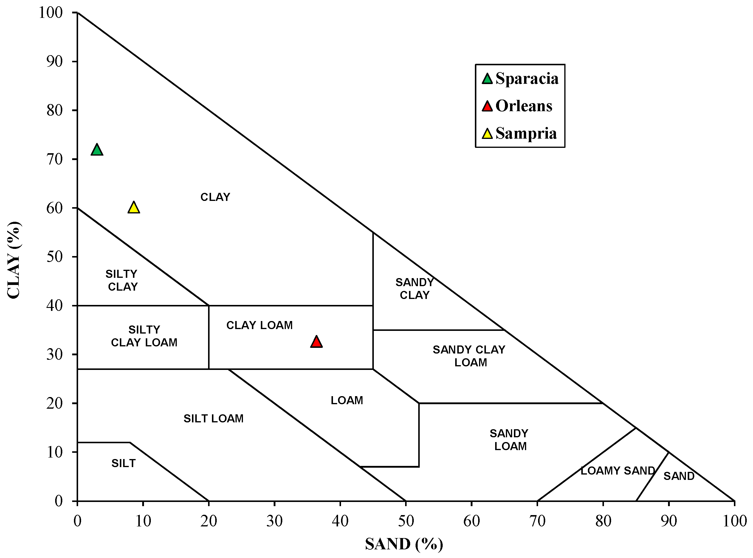
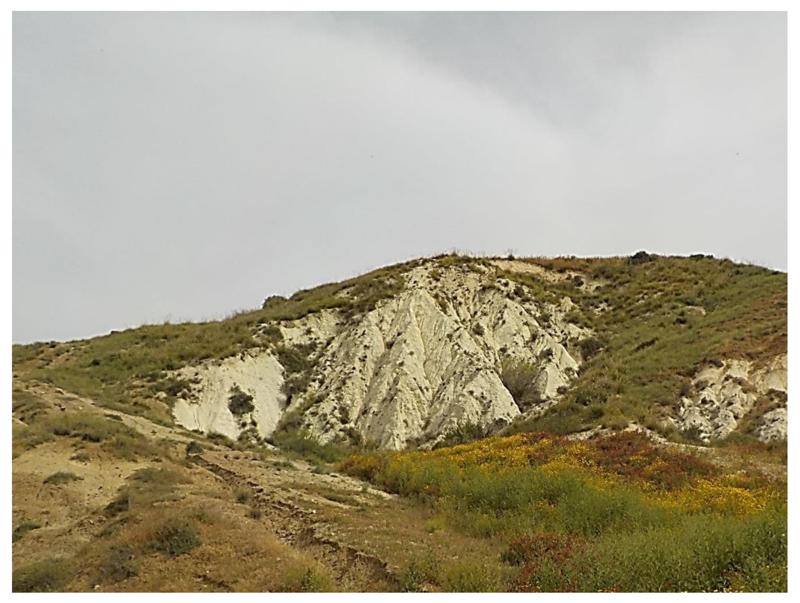
4.1. Soils

In this investigation, three soil samples with different textural characteristics were used. The first sample, named “Sparacia”, was collected in the experimental area located in Western Sicily, Southern Italy, approximately 100 km south of Palermo (37°38′10.27′′ N; 13°45′57.73′′ E). This soil is classified as clay (72% clay, 25% silt, and 3% sand) (Figure 2) and is characterized by a negligible gravel content. Further details on Sparacia soil are listed in Bagarello and Ferro [25] and Bagarello et al. [26].

The soil “Orleans” was collected in the experimental area of the Department of Agriculture, Food and Forest Sciences of the University of Palermo [28,29]. This soil has a clay-loam texture (32.7% clay, 30.9% silt, and 36.4% sand) (Figure 2) and negligible gravel content.

The third soil was collected in the “Sampria” Calanchi area (Figure 2 and Figure 3) located within the Platani river basin, Sicily (Italy) (37.498785° N, 13.848052° E). This soil is classified as clay (60.2% clay, 31.2% silt, and 8.6% sand) and has a negligible gravel content [30]. This area is characterized by heavy erosion processes [31], characterized by narrow channels with a deep V-shaped cross-section and very steep hillslopes. Calanchi landforms disclose well-developed drainage patterns in which erosion channels are separated by sharp knife-edged ridges (Figure 3).

The samples “Sparacia” and “Orleans” have different grain-size distributions, an agricultural land use, and are affected by soil erosion processes. “Sampria” is a degraded soil, due to past intensive erosion processes [32], and a low organic matter content (less than 1%). Agricultural practices in “Sampria” soil are forbidden. In the following, “Sparacia” and “Orleans” soils will be named “non-degraded”, while the soil “Sampria” will be mentioned as “degraded”.

4.2. Samples for the FFC NMR Analyses

The water holding capacity WHC of a soil (i.e., the maximum amount of water that a soil can retain before it starts leaching), was measured to establish a reference water content value of samples to be analyzed by FFC NMR relaxometry. The WHC was adopted as Conte and Ferro [16] established that WHC is the optimal water content to have reliable results (i.e., relaxation times longer than the instrumental switching time of 3 ms). The water holding capacity was measured by using the equipment described in Conte and Ferro [16] and the reliability of the applied procedure was also positively verified by applying the method described in Pohlmeier et al. [23] and Haber-Pohlmeier et al. [33,34].

For each investigated soil, the distribution of T₁ was measured by a sample-to-water ratio of 1:0.25 (w/w) corresponding to the WHC, at a proton Larmor frequency (ν_L) in the range 0.015–35 MHz. Consequently, the tests were carried out by a single value of the soil-to-water ratio and different values of the proton Larmor frequency. The samples were prepared in beakers and then transferred to the NMR tubes to obtain a homogeneous packing.

4.3. FFC NMR Relaxometry and Data Analysis

A Stelar Spinmaster FFC 2000 Fast-Field-Cycling Relaxometer (Stelar s.r.l., Mede, PV–Italy) at a constant temperature of 25 °C was used to carry out all relaxometry measurements. The proton Larmour frequency ν_L corresponding to the relaxation field (BRLX) was changed in the range 0.015–35 MHz by choosing 25 different values. When the ν_L were above 9 MHz, a non-polarized (NP) sequence was applied. Conversely, a pre-polarized (PP) sequence was needed when the proton Larmour frequency was changed for values less than 9 MHz. The PP sequence consists of the application of a polarization magnetic field (B_POL) corresponding to a proton Larmor frequency (ν_L) of 20 MHz for a period (T_POL) of about five times the T₁ estimated at this frequency. After each B_POL, the magnetic field intensity B_RLX was systematically changed. Further details on FFC NMR relaxometry experiments are reported in Conte and Ferro [17].

The Uniform PENalty regularization (UPEN) algorithm [18] was used to achieve the distribution of the longitudinal relaxation times useful to assess HCS.

5. Results

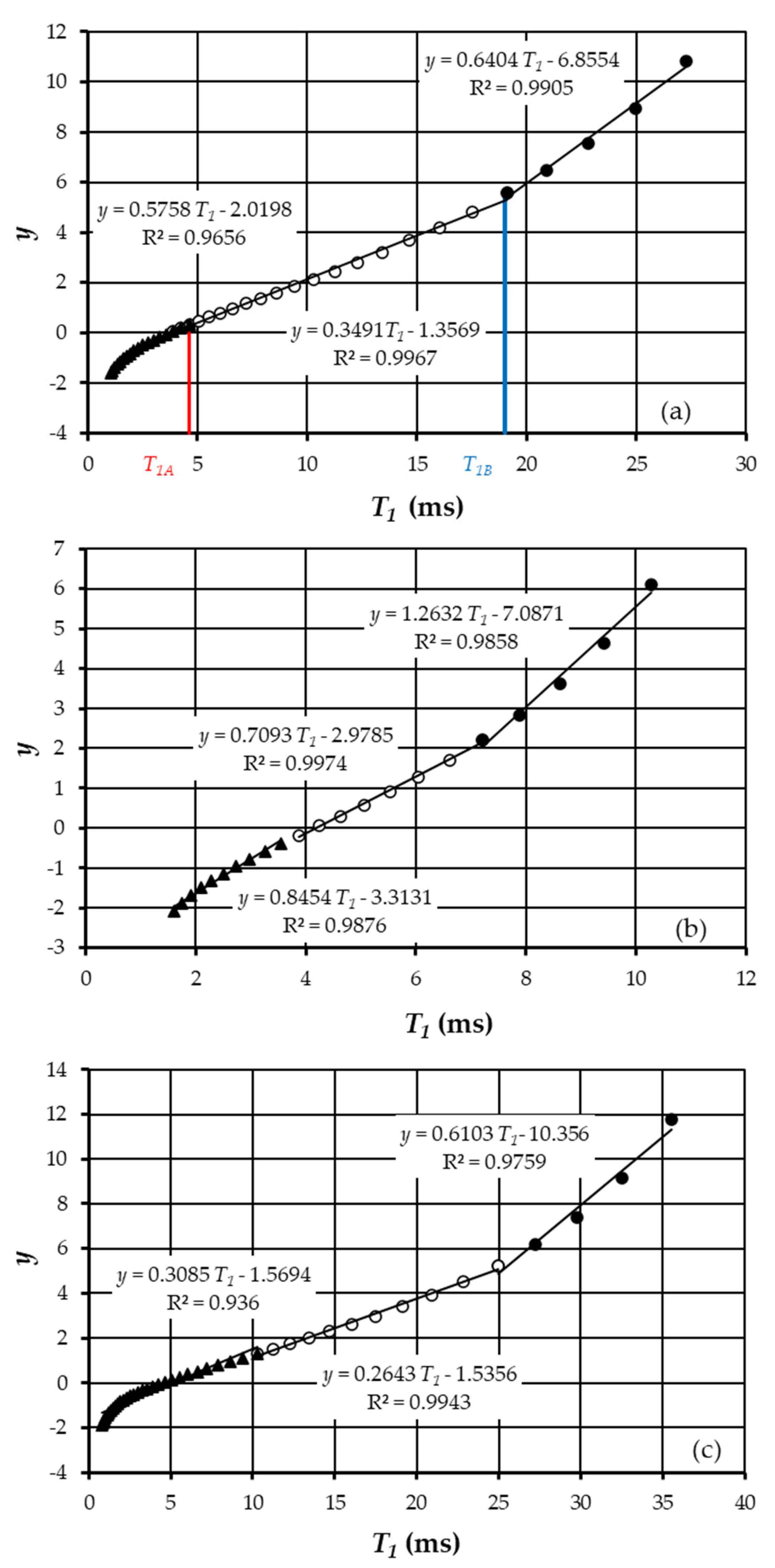
5.1. Plotting the Integral Curve of the Relaxogram in Gumbel’s Diagram

Gumbel’s distribution or Extreme Value Type 1 (EV1) is a double-exponential theoretical probability law [35] which has been applied successfully in many disciplines [36]. Gumbel’s diagram is a plot that allows representing the relationship between the original variable and the corresponding Gumbel’s normalized variable y, which is related to the empirical cumulative frequency of the original variable (Equation (1)).

The integral curve of the relaxogram, i.e., the empirical cumulative frequency distribution F(T₁), was plotted using Gumbel’s diagram, which reports in the x-axis the original variable T₁ and in the ordinate axis the normalized variable y having the following definition:

$$y=-\ln \left(\ln \left(\frac{1}{F\left(T_1\right)}\right)\right)$$

(1)

This diagram represents a different way to plot the pairs (T₁, F(T₁)), i.e., the S-shaped integral curve of the relaxogram. As an example, for the Orleans soil and ν_L = 1 MHz, Figure 4 shows the plot of the pairs (T₁, y) (Figure 4a) and the plot of the second derivative y” of the function y(T₁) (Figure 4b).

The pairs (T₁, y) demonstrate that the function y(T₁) is characterized by three different ranges of T₁ corresponding to three different components, and Figure 4b demonstrates that a flex point (second derivative equal to zero) bounds the low component characterized by the lowest T₁ values. In other words, the point A (Figure 1b), and its abscissa T_1A, can be determined by the flex point (y” = 0) of the integral curve of the relaxogram F(T₁) plotted by Gumbel’s diagram.

In particular, for the Orleans soil and ν_L = 1 MHz, Gumbel’s diagram of Figure 5a shows that the F(T₁) distribution is represented by three straight lines corresponding to three different ranges of T₁: (i) the low component (component 1) occurring for T₁ values less than T_1A = 4.6 ms, (ii) the intermediate component (component 2) corresponding to T₁ values ranging from T_1A = 4.6 ms and T_1B = 19 ms, and (iii) the high component (component 3) corresponding to T₁ values higher than T_1B.

Gumbel’s diagram of Figure 5b shows the F(T₁) distribution for Sampria degraded soil when ν_L = 1 MHz. This figure highlights that F(T₁) distribution is also represented by three straight lines for the degraded soil even if the range of the measured T₁ values (1.6–10 ms) and the corresponding T_1A (3.9 ms) and T_1B (7.2 ms) are less than those of the non-degraded soil (i.e., Orleans). The comparison between Figure 5a,b demonstrated that the F(T₁) distribution of the Sampria sample (i.e., the soil affected by heavy water erosion processes) is displaced on the left side of the F(T₁) distributions obtained for the non-degraded Orleans soil.

For the three investigated soils and some proton Larmor frequencies (ν_L = 0.01, 1, and 3 MHz),

Table 1. Characteristic values of the FFC NMR measurements.

Soil	νL (MHz)	m(T1) (ms)	s(T1) (ms)	G(T1)	T1A (ms)	T1B (ms)	F(T1A)	F(T1B)
Orleans	0.1	4.4	4.3	1.23	4.6	10.3	0.59	0.976
	1	7.5	7.4	1.23	4.6	19.1	0.39	0.996
	3	8.8	9.5	1.35	5.5	24.9	0.39	0.995
Sparacia	0.1	10.3	11.3	1.37	10.3	24.9	0.77	0.983
	1	9.3	9.6	1.28	10.3	24.9	0.76	0.995
	3	10.9	11.4	1.30	9.4	32.5	0.70	0.998
Sampria	0.1	4.6	2.7	0.73	3.5	8.61	0.37	0.992
	1	4.7	2.6	0.70	3.9	7.20	0.38	0.973
	3	4.8	2.4	0.61	4.2	8.61	0.37	0.989

Notes: ν_L = proton Larmor frequency, m(T₁) = mean value of T₁, s(T₁) = standard deviation of T₁, G(T₁) = skewness of T₁, T_1A = relaxation time corresponding to the point A of the F(T₁) distribution, T_1B = relaxation time corresponding to the point B of the F(T₁) distribution, F(T_1A) = empirical cumulative frequency distribution of T_1A, F(T_1B) = empirical cumulative frequency distribution of T_1B.

lists some characteristic values of the FFC NMR measurements: the mean T₁ value, m(T₁), the standard deviation of the measured relaxation times, s(T₁), the skewness, G(T₁), T_1A defining the low component 1 (T₁ < T_1A), T_1B defining the high component 3 (T₁ > T_1B), and the frequency values F(T_1A) and F(T_1B) calculated by the integral curve of the relaxogram of each investigated soil. The values listed in Table 1 allow for stating that: (i) the standard deviation of the relaxation time T₁ of the degraded soil is less than those of the non-degraded soils, confirming that the erosion processes tend to reduce the size variability of soil pores; (ii) for a given ν_L, the relaxation times T_1A and T_1B and the frequency F(T_1A) are characteristic of the investigated soil while the frequency F(T_1B), defining the macro-pore component, is less variable with the soil type and ν_L; and (iii) the F(T₁) distribution of Sampria sample is less skewed than those of the non-degraded soils. Table 1 also shows that all investigated samples are characterized by positive values of skewness G(T₁), i.e., both non-degraded and degraded soil have relaxograms with a tail of distribution extended along the highest T₁ values.

For studying the shape of the integral curve of the relaxogram in Gumbel’s diagram, the measured F(T₁) of the investigated sample was compared with a calculated F(T₁) obtained by a normal distribution, which is characterized by G(T₁) = 0, and mean m(T₁) and standard deviation s(T₁) equal to the measured values listed in Table 1. Therefore, for a given soil at any of the proton Larmor frequencies, the measured F(T₁) (integral curve of the measured relaxogram) is compared with a theoretical F(T₁) having a normal shape with statistical parameters, m(T₁) and s(T₁), equal to the measured values.

As an example, for ν_L = 1 MHz and the Orleans (a) and Sampria (b) samples, Figure 6 reports the comparison between the measured three components’ F(T₁) distribution and those calculated by a normal distribution of the measured relaxation time values.

For both samples, Figure 6 demonstrates that the actual F(T₁) distribution is skewed, presents three components, and cannot be expressed by a symmetric theoretical distribution which should be simply characterized by two components N₁ and N₂. Therefore, the skewed actual F(T₁) distribution is able to represent three pore size classes (micro-, meso-, and macro-pores), while Figure 6 demonstrates that normal and symmetric (G(T₁) = 0) distribution should correspond to a soil in which only two pore size classes could be distinguishable.

The positive skewness of the measured F(T₁) distribution is due to a tail of the relaxogram corresponding to the largest T₁ values and this shape of the relaxogram allow to detect three T₁ ranges which correspond to three pore size classes (micro-, meso-, and macro-pores).

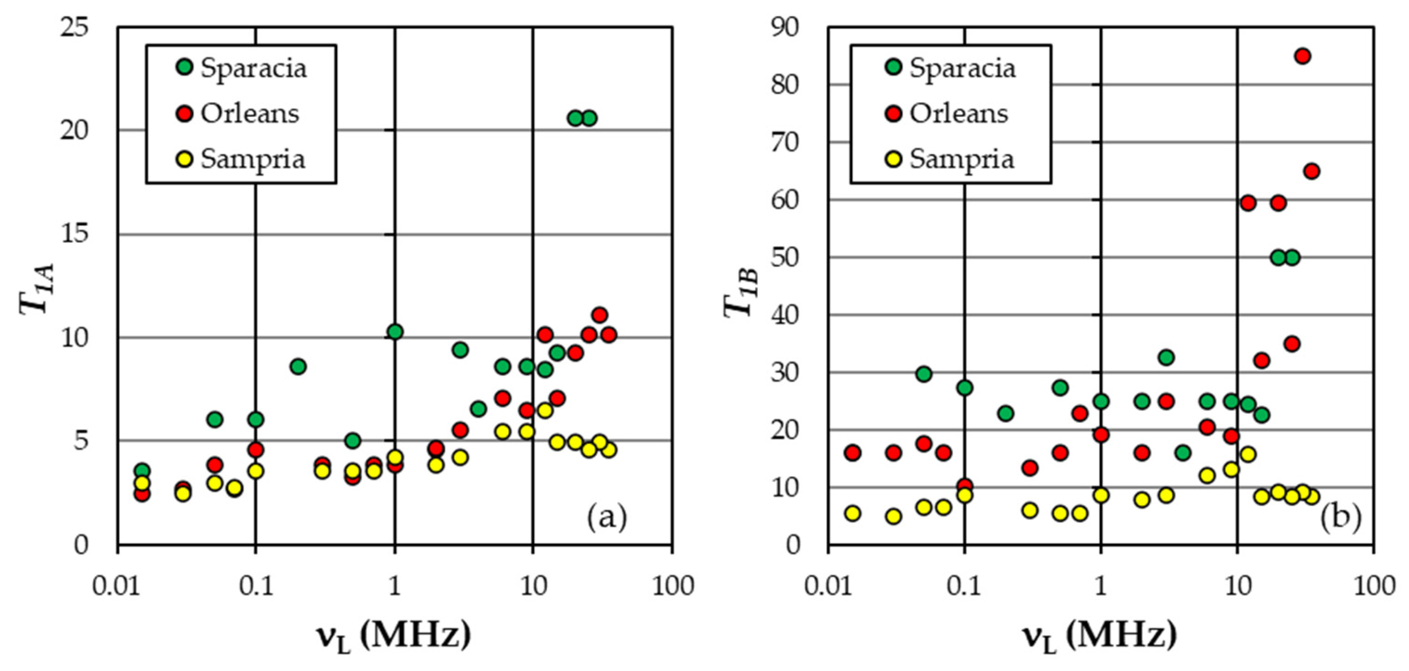
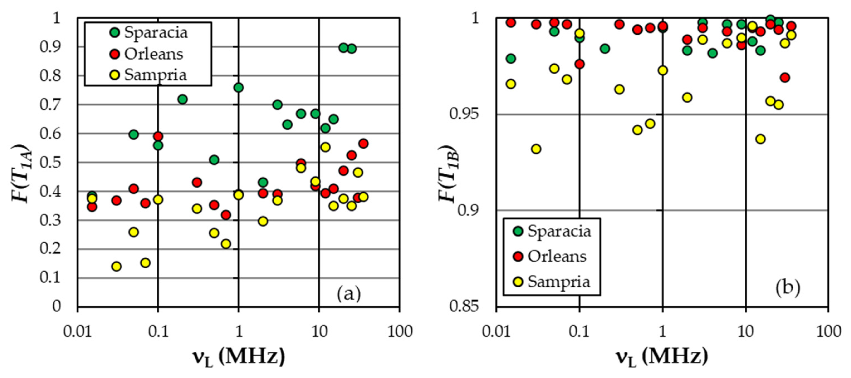
5.2. Characteristic Values of T_1A, T_1B, F(T_1A), and F(T_1B)

For the three investigated soils; Figure 7 shows the characteristic relaxation times T_1A and T_1B vary with ν_L ranging from 0.015 to 35 MHz. This figure shows that the characteristic times T_1A and T_1B and the corresponding frequencies; F(T_1A) and F(T_1B) (Figure 8); present; except for the highest ν_L values (>10 MHz); a poor variability with the proton Larmor frequency. For each investigated soil and ν_L < 10 MHz;

Table 2. Values of the characteristic relaxation times T_1A and T_1B.

Soil	m(T1A)	s(T1A)	m(T1B)	s(T1B)	MFT1A	SFT1A	MFT1B	SFT1B	PMI (%)	PME (%)	PMA (%)
Orleans	4.24	1.39	17.50	3.98	0.405	0.072	0.993	0.006	40.5	58.8	0.7
Sparacia	7.04	2.18	24.64	5.03	0.603	0.121	0.990	0.007	60.3	38.7	1.0
Sampria	3.74	0.92	7.69	2.55	0.313	0.104	0.968	0.019	31.3	65.5	3.2

Notes: m(T_1A) = mean value of T_1A, s(T_1A) = standard deviation of T_1A, m(T_1B) = mean value of T_1B, s(T_1B) = standard deviation of T_1B, MFT_1A = mean value of F(T_1A), SFT_1A = standard deviation of F(T_1A), MFT_1B = mean value of F(T_1B), SFT_1B = standard deviation of F(T_1B), PMI percentage of micro-pores, PME percentage of meso-pores, PMA percentage of macro-pores.

lists the mean values and the standard deviation of the characteristic times T_1A and T_1B and the corresponding frequencies; F(T_1A) and F(T_1B). The values listed in Table 2 demonstrate that: (i) the relaxation time T_1A and T_1B are; on average; affected by soil type; and the minimum values are characteristics of the degraded soil; (ii) the frequency F(T_1A) is; on average; dependent on soil type and this result is justified taking into account that this frequency corresponds to the percentage of micro-pores of the investigated sample; and (iii) the frequency F(T_1A) is; on average; independent of the investigated soil type and varies in a very narrow range (0.968-0.993)

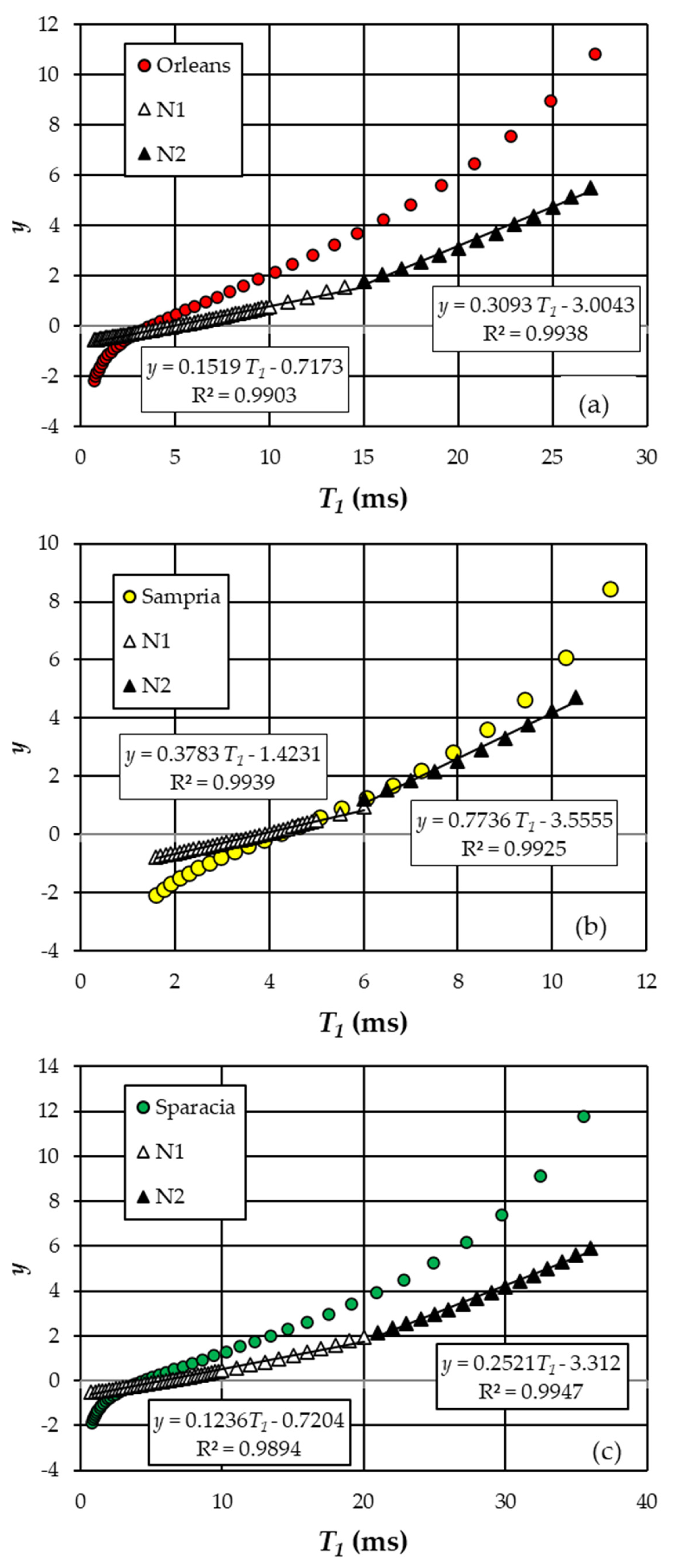
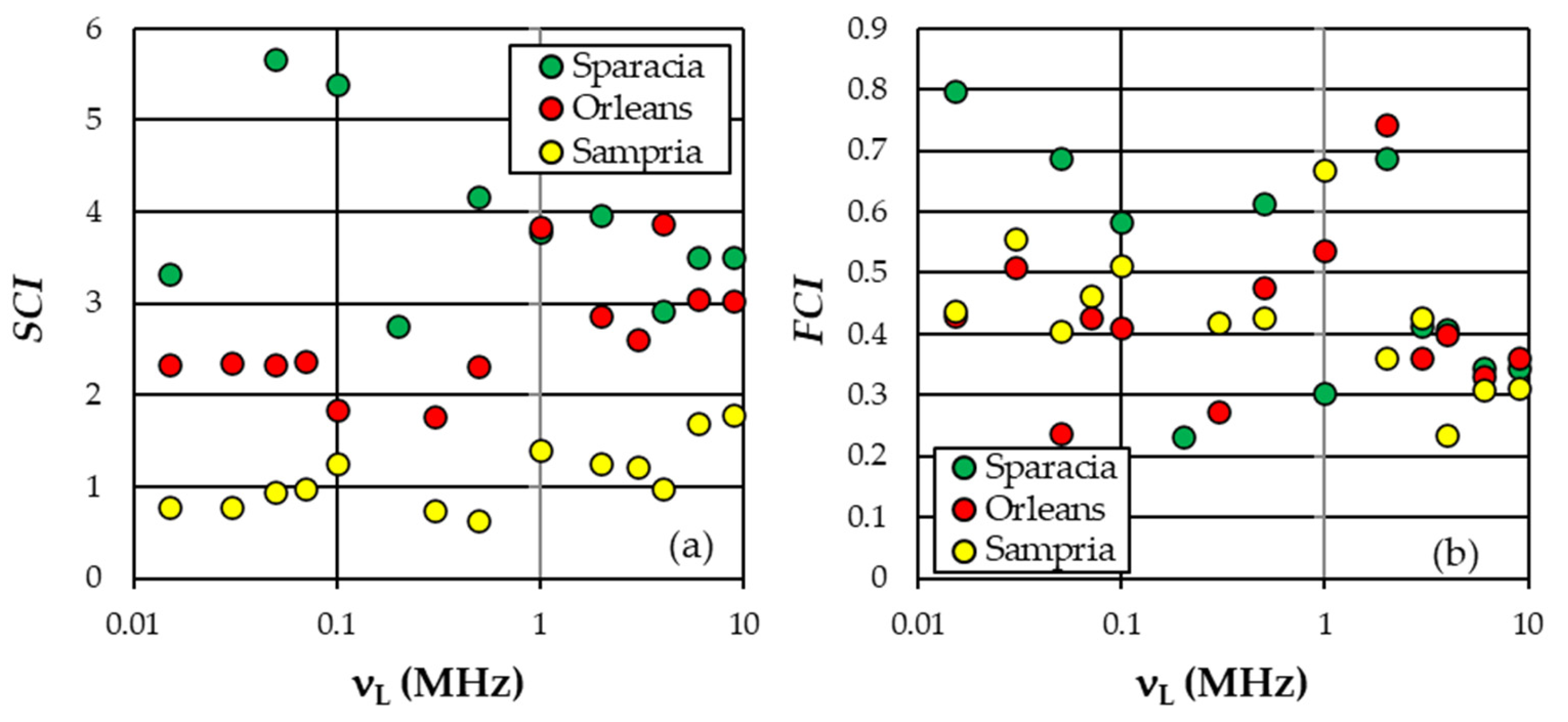
5.3. Definition of the Structural and Functional Connectivity Indices

By considering that the F(T₁) distribution plotted in Gumbel’s diagram (Figure 5) is represented by three straight lines corresponding to three different ranges of T₁, the slope of each component (S₁ for the low component 1, S₂ for the intermediate component 2, and S₃ for the high component 3) can be used to propose a new definition of the SCI and FCI indices.

In particular, the intermediate component (component 2) corresponds to the limb zone AB of the frequency distribution F(T₁) (Figure 1b) and can be used to calculate the structural connectivity index, SCI. In fact, according to Conte and Ferro [15], this choice is supported by the circumstance that the central range of T₁ values (T_1B−T_1A) is representative of the main structure of the soil. In other words, the interval (T_1B−T_1A), corresponding to water molecules moving in meso-pores, can be used to represent the spatial pattern inside the soil. According to the relationship between the relaxation time and the pore-size, the structural connectivity index, SCI, can be defined as:

$$SCI=\frac{1}{S_2}$$

(2)

For the functional component of hydrological connectivity inside the soil, the low component 1 and the high component 3 of F(T₁) have to be considered. In fact, the component 3 corresponds to T₁ values higher than T_1B, thereby representing water blocked in larger pores (unconstrained water molecules), while component 1 corresponds to T₁ < T_1A and water molecules trapped in smaller pores. As a consequence, the functional connectivity index FCI can be defined as:

$$FCI=\frac{S_1}{S_3}$$

(3)

For the three investigated soils, Figure 9 shows as SCI and FCI vary with ν_L in the range 0.015–35 MHz. Figure 9a demonstrates that the structural connectivity of a degraded soil (Sampria) is less than that of the investigated non-degraded soil as an increase of the slope S₂ corresponds to a decrease of the range of frequencies F(T₁) associated to the intermediate component, i.e., the percentage of meso-pores in the overall pore size distribution decreases. The mean value of SCI is equal to 3.96 (+0.93) for the Sparacia soil and decreases to 2.66 (±0.66) and 1.07 (±0.36) for the Orleans and Sampria soil, respectively. Figure 9b shows that no clear trend of FCI with proton Larmour frequency and soil type can be easily inferred for the investigated samples. However, the mean value of FCI is equal to 0.49 (±0.19) for the Sparacia soil and decreases to 0.42 (±0.13) and 0.39 (±0.10) for the Orleans and Sampria soil, respectively. Moreover, the empirical cumulative frequency distribution of FCI plotted in Figure 10 highlights that the frequency distribution of FCI, especially for FCI > 0.5, of a degraded soil is nearest to the frequency axis than non-degraded soils, confirming that the lowest functional connectivity characterizes a degraded soil.

For the investigated soils and three values of the proton Larmor frequency,

Table 3. Characteristic data of functional and structural components of HCS.

Soil	νL (MHz)	S1	S3	SCI	FCI	PMI (%)	PME (%)	PMA (%)
Orleans	0.1	0.5741	1.0906	1.84	0.41	59	38.6	2.4
	1	0.3847	0.6404	3.84	0.54	39	60.6	0.4
	3	0.2811	0.6640	2.61	0.36	39	60.5	0.5
Sparacia	0.1	0.3347	0.3617	5.39	0.58	77	21.3	1.7
	1	0.3085	0.6103	3.78	0.30	76	23.5	0.5
	3	0.3240	0.6042	4.54	0.41	70	28.8	1.2
Sampria	0.1	0.9485	1.4911	1.26	0.51	37	62.2	0.8
	1	0.8454	1.2632	0.86	0.21	38	59.3	2.7
	3	0.9270	1.6645	1.21	0.43	37	61.9	1.1

Notes: ν_L = proton Larmor frequency, S₁ = slope of the low component 1 of the F(T₁) distribution in the Gumbel plot, S_{3 =} slope of the high component 3 of the F(T₁) distribution in the Gumbel plot, SCI = structural connectivity index, FCI = functional connectivity index, PMI percentage of micro-pores, PME percentage of meso-pores, PMA percentage of macro-pores.

lists the value of the percentage of micro-pores, PMI, meso-pores, PME, and macro-pores, PMA detected by NMR measurements. In particular, the percentages were obtained by the following relationships:

$$PMA=100 \left[1-F\left(T_{1B}\right)\right]$$

(4)

$$PME=100 \left[F\left(T_{1B}\right)-F\left(T_{1A}\right)\right]$$

(5)

$$PMI=100-PMA-PMI$$

(6)

6. Discussion

6.1. Plotting the Integral Curve of the Relaxogram in Gumbel’s Diagram

As the F(T₁) distribution of Sampria soil is generally shifted towards shorter T₁ values (Figure 5) the erosion processes determine a reduction of the macropore size, consequently leading to a larger number of meso-pores and micro-pores [15]. Water molecules move faster in macropores than in meso- and micropores and a decrease of T₁ values corresponds to a disappearance of macropores and an increase of the number of meso- and micro-pores. Thereby, the degraded Sampria soil has also limited functional connectivity.

The relaxation time distribution of the degraded Sampria soil (Figure 6) is characterized by a shape that is more symmetric (G(T₁) in the range 0.61–0.73) as compared to the non-degraded soils (G(T₁) in the range 1.23–1.37), and this shape can be physically justified by considering the degraded soil sample has a more uniform pore size distribution dominated by micro- and meso-pores, making molecular motions difficult, and therefore, providing the shortest T₁ values [15]. Figure 6b demonstrates that the actual measured F(T₁) distribution of Sampria soil, in comparison with the non-degrades Orleans soil (Figure 6a), is nearer to the normal distribution as the intense erosion processes tend to reduce the size of the soil macro-pores [15] and to have an overall pore size distribution more uniform. The degraded soil sample (Figure 6b) presents a relaxogram shape that is near to a theoretical F(T₁) distribution in which the micro and meso-pores belong to the same pore size class; in other words, the intense erosion processes simplify the structure of the soil sample and the pore-size distribution is more similar to a two classes distribution.

6.2. Characteristic Values of T_1A, T_1B, F(T_1A), and F(T_1B)

The mean values of the relaxation time T_1A, listed in Table 2, demonstrate that this variable is representative of the soil type and this circumstance can be justified considering that T_1A is useful to establish the micro-pore component of the soil. The corresponding frequency value F(T_1A) varies with the soil type with a percentage of micro-pores (40.5% for the Orleans soil and 60.3% for the Sparacia soil) which increases with soil clay content (32.7% for Orleans and 72% for Sparacia). For the investigated soils, the Sampria sample has the minimum percentage of micro-pores of 31.3% and the maximum percentage of meso-pores (65.5%). This result can be justified by considering that the erosion process is selective, and the flow tends to transport small-size particles determining an eroded soil that has a coarser grain-size distribution than the original soil. The coarsening of the particle sizes of eroded soils is associated with an increase in the meso-pore class.

The mean values of the relaxation time T_1B point out that all investigated soils are characterized by a low percentage of sand (in the range 3–36.2%) which justifies the low percentage of macro-pores. The frequency value F(T_1B) corresponds to investigated soil types which are dominated by the presence of micro- and meso-pores with a percentage of 97–99%. In other words, for the investigated natural soils, a single value of 0.99 can be assumed as representative and can be used to individuate the point B in the integral relaxogram curve.

In previous studies [15,16,17] the position of the points A and B on the F(T₁) frequency distribution were arbitrarily selected using the frequency values equal to 0.01 for the point A and F(T₁) = 0.99 for the point B. The analysis developed in this paper demonstrated that the original criterion used by Conte and Ferro [15] for stating the position of the B point is coincident with that individuated by Gumbel’s diagram which is obtained considering the third component of the S-shaped F(T₁) frequency distribution. The arbitrary position of the point A chosen by Conte and Ferro [15] was not verified by the analysis developed in this paper as the first component is defined by a F(T_1A) value which is always higher than 0.01 and is dependent on the soil type. This last result is impressive from a physical point of view as the percentage of micro-pore existing in a soil sample is related to the grain-size distribution.

6.3. Definition of the Structural and Functional Connectivity Indices

Figure 9 shows that the structural connectivity is affected by soil degradation as the SCI of degraded soil (Sampria) is less than that of the investigated non-degraded soils. In other words, the intense erosion processes acting on Sampria calanchi area resulted in a different macro-pore distribution in comparison with non-degraded soils. This result confirms that the proposed SCI index obtained by the NMR technique is able to distinguish the low structural connectivity of degraded soils from that of non-degraded ones [17]. The SCI value of 1.07 for the degraded Sampria soil is appreciably less than the range (2.66–3.96) of non-degraded investigated soils. Figure 10 allows for establishing that degraded soil is also characterized by the lowest values of functional connectivity. This result can be justified by considering that the F(T₁) curve of the degraded Sampria soil has a quasi-uniform shape [15] corresponding to a quasi-uniform pore size distribution in which micro- and meso-pores prevail. This pore-size distribution, allowing restriction of water dynamics because of strong interactions with pore walls, provides the shortest relaxation times and is associated with a small SCI value. Moreover, as intense soil erosion processes affect the Sampria soil, the size of the soil macro-pores is reduced [15], and this condition limits soil functional connectivity.

The values of PMI, PME, and PMA listed in Table 3 for the investigated soils indicate that all samples are characterized by a low percentage of macro-pores, Sparacia soil having the high clay percentage is also characterized by the highest percentage of micro-pores, and the highest percentage of meso-pores correspond to Orleans soil having a clay-loam texture (32.7% clay, 30.9% silt, and 36.4% sand).

When the soil is characterized by a single component corresponding to the meso-pore size, the F(T₁) distribution in Gumbel’s diagram is represented by a single straight line having a slope S₁ = S₂ = S₃. If the three slopes S₁, S₂, and S₃ are coincident (i.e., S₁ = S₃ = S₂), the absence of micro-pore and macro-pore components determines, according to the definition of FCI (Equation (3)), a value of FCI equal to 1. In this condition (FCI = 1), according to the definition of SCI (Equation (2)), the following relationship is obtained:

$$SCI=\frac{1}{S_2}=\frac{y_{1max}-y_{1min}}{T_{1max}-T_{1min}}$$

(7)

in which T_1max is the maximum measured T₁ value, T_1min is the minimum measured T₁ value, y_1max and y_1min are the y values calculated by Equation (1) for the frequency values corresponding to T_1max and T_1min.

7. Conclusions

Using the results of previous papers [14,15,16,17,18], this study presents a new quantitative definition of the structural (SCI) and functional (FCI) connectivity indices. The proposed new representation of the relaxogram integration curve allowed for distinguishing three linear components, corresponding to three different relaxation time ranges, characterized by three different slopes, and these slope values were used to redefine the SCI and FCI indices.

In particular, the results showed that the two points, identified in Gumbel’s diagram by the abrupt slope changes of the relaxogram integration curve, are useful to establish two characteristic relaxation times, T_1A and T_1B, which allow for defining three well-known pore size classes (T₁ < T_1A micro-pores, T_1A < T₁ < T_1B meso-pores, and T₁ > T_1B macro-pores). For each investigated sample, the analysis demonstrated that the frequency values F(T_1A) and F(T_1B) obtained by the relaxogram integration curve are dependent on the applied Proton Larmor frequency, and the relaxogram can be used to determine the pore-size ranges of the investigated sample.

The developed analysis also established that the lowest SCI values correspond to soils characterized by erosion processes, while the difference in FCI values between non-degraded and degraded soils is more restrained. In particular, this analysis confirmed that degraded and non-degraded soils have different grain size distributions determining differences in SCI values.

Further experiments with soil samples with different textures are required to both confirm that the relaxogram can be used to determine the pore-size ranges of the investigated samples and the new proposed definition of the Structural Connectivity and Functional Connectivity Index.

References

1. Marchamalo, M.; Hooke, J.M.; Sandercock, P.J. Flow and Sediment Connectivity in Semi-arid Landscapes in SE Spain: Patterns and Controls. Land Degrad. Dev. 2016, 27, 1032–1044. [Google Scholar] [CrossRef]
2. Keesstra, S.D.; Bagarello, V.; Ferro, V.; Finger, D.; Parsons, A.J. Connectivity in hydrology and sediment dynamics. Land Degrad. Dev. 2020, 31, 2525–2528. [Google Scholar] [CrossRef]
3. Pringle, C. What is hydrologic connectivity and why is it ecologically important? Hydrol. Process. 2003, 17, 2685–2689. [Google Scholar] [CrossRef]
4. Bracken, L.J.; Wainwright, J.; Ali, G.A.; Tetzlaff, D.; Smith, M.W.; Reaney, S.M.; Roy, A.G. Concepts of hydrological connectivity: Research approaches, Pathways and future agendas. Earth Sci. Rev. 2013, 119, 17–34. [Google Scholar] [CrossRef] [Green Version]
5. Reaney, S.M.; Bracken, L.J.; Kirkby, M.J. The importance of surface controls on overland flow connectivity in semi-arid environments: Results from a numerical experimental approach. Hydrol. Process. 2014, 28, 2116–2128. [Google Scholar] [CrossRef] [Green Version]
6. López-Vicente, M.; Nadal-Romero, E.; Cammeraat, E.L.H. Hydrological Connectivity Does Change Over 70 Years of Abandonment and Afforestation in the Spanish Pyrenees. Land Degrad. Dev. 2017, 28, 1298–1310. [Google Scholar] [CrossRef] [Green Version]
7. Wu, Y.; Zhang, Y.; Dai, L.; Xie, L.; Zhao, S.; Liu, Y.; Zhang, Z. Hydrological connectivity improves soil nutrients and root architecture at the soil profile scale in a wetland ecosystem. Sci. Total. Environ. 2021, 762, 143162. [Google Scholar] [CrossRef]
8. Wainwright, J.; Turnbull, L.; Ibrahim, T.G.; Lexartza-Artza, I.; Thornton, S.F.; Brazier, R.E. Linking environmental régimes, space and time: Interpretations of structural and functional connectivity. Geomorphology 2011, 126, 387–404. [Google Scholar] [CrossRef]
9. Belisle, M. Measuring landscape connectivity: The challenge of behavioural landscape ecology. Ecology 2005, 86, 1988–1995. [Google Scholar] [CrossRef] [Green Version]
10. Turnbull, L.; Wainwright, J.; Brazier, R.E. A conceptual framework for understanding semi-arid land degradation: Ecohydrological interactions across multiple-space and time scales. Ecohydrology 2008, 1, 23–34. [Google Scholar] [CrossRef] [Green Version]
11. Uezu, A.; Metzger, J.P.; Vielliard, J.M.E. Effects of structural and functional connectivity and patch size on the abundance of seven Atlantic forest bird species. Biol. Conserv. 2005, 123, 507–519. [Google Scholar] [CrossRef]
12. Bracken, J.; Croke, J. The concept of hydrological connectivity and its contribution to understanding runoff-dominated geomorphic systems. Hydrol. Process 2007, 21, 1749–1763. [Google Scholar] [CrossRef]
13. Baartman, J.E.M.; Masselink, R.; Keesstra, S.D.; Temme, A.J.A.M. Linking landscape morphological complexity and sediment connectivity. Earth Surf. Process. Landf. 2013, 38, 1457–1471. [Google Scholar] [CrossRef]
14. Conte, P.; Di Stefano, C.; Ferro, V.; Laudicina, V.A.; Palazzolo, E. Assessing hydrological connectivity inside a soil by fast-field-cycling nuclear magnetic resonance relaxometry and its link to sediment delivery processes. Environ. Earth Sci. 2017, 76, 526. [Google Scholar] [CrossRef]
15. Conte, P.; Ferro, V. Measuring hydrological connectivity inside a soil by low field nuclear magnetic resonance relaxometry. Hydrol. Process. 2018, 32, 93–101. [Google Scholar] [CrossRef]
16. Conte, P.; Ferro, V. Standardizing the use of fast-field cycling NMR relaxometry for measuring hydrological connectivity inside the soil. Magn. Reson. Chem. 2020, 58, 41–50. [Google Scholar] [CrossRef]
17. Conte, P.; Ferro, V. Measuring hydrological connectivity inside soils with different texture by fast field cycling nuclear magnetic resonance relaxometry. Catena 2022, 209, 105848. [Google Scholar] [CrossRef]
18. Conte, P. Environmental Applications of Fast Field-cycling NMR Relaxometry. In Field-Cycling NMR Relaxometry: Instrumentation, Model Theories and Applications; Kimmich, R., Ed.; The Royal Society of Chemistry: Croydon, UK, 2019; pp. 229–254. [Google Scholar]
19. Conte, P.; Lo Meo, P. Nuclear Magnetic Resonance with Fast Field-Cycling Setup: A Valid Tool for Soil Quality Investigation. Agronomy 2020, 10, 1040. [Google Scholar] [CrossRef]
20. Jaeger, F.; Bowe, S.; Schaumann, G.E. Evaluation of 1H NMR relaxometry for the assessment of pore size distribution in soil samples. Eur. J. Soil Sci. 2009, 60, 1052–1064. [Google Scholar] [CrossRef]
21. Meyer, M.; Buchmann, C.; Schaumann, G.E. Determination of quantitative pore-size distribution of soils with 1H NMR relaxometry. Eur. J. Soil Sci. 2018, 69, 393–406. [Google Scholar] [CrossRef]
22. Novotny, E.H.; deAzevedo, E.R.; de Godoy, G.; Consalter, D.M.; Cooper, M. Determination of soil pore size distribution and water retention curve by internal magnetic field modulation at low field 1H NMR. Geoderma 2023, 431, 116363. [Google Scholar] [CrossRef]
23. Pohlmeier, A.; Haber-Pohlmeier, S.; Stapf, S. A Fast Field Cycling Nuclear Magnetic Resonance Relaxometry Study of Natural Soils. Vadose Zone J. 2009, 8, 735–742. [Google Scholar] [CrossRef]
24. Pagliai, M.; Vignozzi, N. The soil pore system as an indicator of soil quality. In Sustainable Land Management-Environmental Protection. A Soil Physical Approach; Pagliai, M., Jones, R., Eds.; Advances in GeoEcology, Catena Verlag; IUSS: Reiskirchen, Germany, 2002; pp. 71–82. [Google Scholar]
25. Bagarello, V.; Ferro, V. Plot-scale measurement of soil erosion at the experimental area of Sparacia (southern Italy). Hydrol. Process 2004, 18, 141–157. [Google Scholar] [CrossRef]
26. Bagarello, V.; Di Piazza, G.V.; Ferro, V.; Giordano, G. Predicting unit plot soil loss in Sicily, south Italy. Hydrol. Process. 2008, 22, 586–595. [Google Scholar] [CrossRef]
27. Hillel, D. Environmental Soil Physics; Academic Press: New York, NY, USA, 1998. [Google Scholar]
28. Carollo, F.G.; Di Stefano, C.; Nicosia, A.; Palmeri, V.; Pampalone, V.; Ferro, V. Flow resistance in mobile bed rills shaped in soils with different texture. Eur. J. Soil Sci. 2021, 72, 2062–2075. [Google Scholar] [CrossRef]
29. Di Stefano, C.; Nicosia, A.; Palmeri, V.; Pampalone, V.; Ferro, V. Rill flow resistance law under sediment transport. J. Soils Sediments 2022, 22, 334–347. [Google Scholar] [CrossRef]
30. Caraballo-Arias, N.A.; Conoscenti, C.; Di Stefano, C.; Ferro, V. Testing GIS-morphometric analysis of some Sicilian badlands. Catena 2014, 113, 370–376. [Google Scholar] [CrossRef]
31. Phillips, C.P. The badlands of Italy: A vanishing landscape? Appl. Geogr. 1998, 18, 243–257. [Google Scholar] [CrossRef]
32. Caraballo-Arias, N.A.; Di Stefano, C.; Ferro, V. Morphological characterization of calanchi (badland) hillslope connectivity. Land Degrad. Dev. 2017, 29, 1190–1197. [Google Scholar] [CrossRef]
33. Haber-Pohlmeier, S.; Stapf, S.; Pohlmeier, A. NMR Fast Field Cycling Relaxometry of Unsaturated Soils. Appl. Magn. Reson. 2014, 45, 1099–1115. [Google Scholar] [CrossRef]
34. Haber-Pohlmeier, S.; Stapf, S.; Van Dusschoten, D.; Pohlmeier, A. Relaxation in a Natural Soil: Comparison of Relaxometric Imaging, T 1-T 2 Correlation and Fast-Field Cycling NMR. Open Magn. Reson. J. 2010, 3, 57–62. [Google Scholar] [CrossRef]
35. Gumbel, E.J. Statistics of Extremes; Columbia University Press: New York, NY, USA, 1958. [Google Scholar]
36. Santner, J.F. An Introduction to Gumbel or Extreme Value Probability Paper; EPA-430/1-73-016; US Environmental Protection Agency, Water Programs Operations: Cincinnati, OH, USA, 1973. [Google Scholar]
Figure 1. Example of distribution of the longitudinal relaxation time (a) with the corresponding empirical cumulative frequency F(T1) (b).
Water 15 02397 g001
Figure 2. Texture of the investigated soils [27].
Water 15 02397 g002
Figure 3. The “Sampria” experimental area.
Water 15 02397 g003
Figure 4. Pairs (T1, y) (a) and (T1, y”) (b) corresponding to a proton Larmor frequency of 1 MHz and the empirical cumulative frequency F(T1) distribution of the Orleans soil.
Water 15 02397 g004
Figure 5. Pairs (T1, y) corresponding to the empirical cumulative frequency F(T1) S-shaped distribution of the Orleans (a), Sampria (b), and Sparacia (c) soils for a proton Larmor frequency of 1 MHz.
Water 15 02397 g005
Figure 6. Comparison, for a proton Larmor frequency of 1 MHz, between the measured cumulative frequency F(T1) and the theoretical F(T1) having a normal shape (N1 and N2) for the Orleans (a), Sampria (b), and Sparacia (c) investigated samples.
Water 15 02397 g006
Figure 7. Relationship, for the investigated soils, between the relaxation times T1A (a), T1B (b), and the proton Larmour frequency.
Water 15 02397 g007
Figure 8. Relationship, for the investigated soils, between the empirical cumulative frequency F(T1A) (a), F(T1B) (b), and the proton Larmor frequency.
Water 15 02397 g008
Figure 9. Relationship, for the investigated soils, between the structural connectivity index SCI (a), the functional connectivity index FCI (b), and the proton Larmor frequency.
Water 15 02397 g009
Figure 10. Empirical frequency cumulative distribution of the functional connectivity index FCI for the investigated soils.
Water 15 02397 g010