Energy Transfer and Reverse Flow Characteristics in the Interaction Process between Non-Breaking Solitary Wave and a Steep Seawall: A Case Study

Abstract

This study utilized a two-dimensional numerical viscous wave tank to simulate the run-up and run-down processes of non-breaking solitary waves on a steep seawall. The research aimed to investigate the transformation between wave potential energy and kinetic energy, the evolution mechanisms of the wave and flow fields, and the correlation between the dynamic pressure gradient and the reverse flow near the sloping bed. The numerical model results were consistent with laboratory measurements of free surface elevations and flow velocity profiles, demonstrating the accuracy of the numerical model. This study focused on a solitary wave with a wave-height-to-water-depth ratio of 0.15, propagating on a representative seawall with a steep slope of 1:3 along the western coast of Taiwan. The simulation results indicate that the maximum run-up height occurs when the potential energy is at its highest. Undertow is caused by the adverse pressure gradient within the flow field, and the dynamic pressure on the sloping bed is directly proportional to the free surface elevation. Therefore, by observing the spatial changes in the free surface elevation, we can indirectly determine the occurrence time of undertow.

1. Introduction

The interactions between waves and structures during the wave propagation process are complex. The accompanying complex wave–structure interaction, wave pressure forces, and bottom shear stress play a significant role in the design of coastal structures such as seawalls, as well as having an impact on scouring in front of seawall toes.

The long waves brought by typhoons or tsunamis triggered by undersea earthquakes are often similar to solitary waves in terms of their characteristics. They typically have single-wave peaks and relatively simple flow fields, which makes them easier to study and understand than harmonic waves. Therefore, early researchers conducted many experiments on the run-up of solitary waves on steeply sloping beds to investigate the behavior of long waves attacking nearshore seawalls. By simplifying the complexity of the research problem in this manner, it will be beneficial for fundamental studies on wave–structure interactions.

Solitary waves, also known as solitons, are nonlinear waves that can travel long distances without changing their shape or speed. The Carrier–Greenspan theory [1] has been widely used in the analytical study of solitary waves. This theory is based on the non-linear shallow water (NLSW) equation, which can describe the changes in the shape and speed of solitary waves as they propagate in shallower waters [2,3]. Ref. [4] measured the maximum run-up height of solitary waves on sloping beaches, and studied the relationship between maximum run-up height and wave-height-to-water-depth ratio. With the advancement of experimental equipment and measurement techniques, high-speed cameras have been used to record the changes in the free surface during the run-up and overtopping of solitary waves. Similar studies include [5,6].

The factors that affect the run-up of solitary waves include incidence conditions, slope grade, and the roughness of the contact surface, among others. An excessive number of parameters tends to complicate the theoretical solution process. Consequently, many early analytical solutions focused on studying wave run-up before wave breaking [1,7,8,9,10,11,12]. Ref. [13] used shallow water wave equations to derive run-up changes in solitary waves on inclining slopes. Comparisons of the theoretical solutions and the experimental results indicate that linear shallow water wave equations were sufficient to derive the maximum run-up height of solitary waves. However, NLSW wave equations were found to describe the run-up process of solitary waves on inclining slopes more completely than linear equations. The studies conducted by [14,15,16] are other examples involving the use of NLSW wave equations to solve run-up problems.

Considering the effects of wave height, wave steepness, and breaking waves, Ref. [17] used the perturbation method to solve the NLSW wave equation and approximate the maximum run-up in the swash zone. Their estimation results were consistent with the run-up law proposed by [18], validating the applicability of their approach in predicting run-up. Ref. [19] proposed an energy balance model (EBM) based on the principle of conservation of energy, taking into account the dissipation of energy during wave breaking and neglecting factors such as bottom friction. Through experimental calibration, the model can be used to rapidly estimate the relationship between the maximum run-up height and the wave-height-to-water-depth ratio under different slope conditions.

Most previous studies have focused on measuring the maximum run-up height. However, when an incident solitary wave interacts with a slope, free surface deformation and energy dissipation occur, making it difficult to gain a comprehensive understanding of the entire water movement by observing changes in run-up height alone. In order to visualize the actual flow field, other studies have employed particle image velocimetry (PIV) technology, which combines digital image processing and flow visualization, as well as laser Doppler velocimetry (LDV), which allows for single-point measurement, to display the run-up and run-down flow fields. In an experimental tank, Ref. [20] generated incident solitary waves with a wave-height-to-water-depth ratio of 0.17 in the upstream section of the flume and propagated them towards a downstream sloping bed with the steep slope s = 1:1.732. Using PIV technology, they captured the free surface changes in the solitary waves on the slope and analyzed the velocity of underwater particles. Ref. [21] also used PIV to examine the flow field changes in the swash zone during the incidence of nonlinear solitary waves on an inclining seabed. Ref. [22] employed a laser to measure the surface line of water bodies on slopes in swash zones and investigate the three-dimensional run-up and turbulence caused by tsunamis near the coast. Ref. [23] conducted an experimental investigation using high-speed particle image velocimetry (HSPIV) to observe the evolution of the flow field of a non-breaking solitary wave propagating over a 1:3 sloping beach in a laboratory setting. The study aimed to explore the correlation between the flow separation and reverse flow phenomena at the bottom of the slope and the distribution of acceleration fields and pressure gradients during the run-up and run-down phases. Despite the maturity and high visualizability of PIV, the wide-angle lenses of cameras often limit the observation range. To achieve comprehensive image capture in experimental tanks, multiple image averaging or camera movement is required. Numerical models can fill this gap. After verifying the accuracy of the models, researchers can comprehensively study the flow field changes during the wave–structure interaction process or the entire energy evolution process.

Common numerical models used for simulating the interaction between waves and coastal structures are the depth-averaged and the Reynolds-averaged Navier–Stokes (RANS) methods. The basic theory of depth-averaged methods is to reduce the spatial scale by a dimension through depth integration, such as the NLSW wave equation or the Boussinesq equation (BE). The NLSW wave equation is suitable for shallow water areas, and its nonlinear convective term and bottom friction have a significant impact on simulating the shoaling process of waves near the coast. Many researchers, such as [24,25,26,27,28], have used these equations to simulate the run-up process of solitary waves and studied the relationship between run-up height and given water depths and slope angles. Subsequently, Ref. [29] extended the study to three-dimensional run-up analysis.

The NLSW wave equation assumes a uniform distribution of the flow field in the vertical direction, thereby neglecting the effects of dispersion. On the other hand, the BEs use a polynomial approximation of the flow field in the vertical direction, allowing for the retention of the nonlinear term and resulting in a flow field under non-static pressure distribution. The typical BEs [30] utilize a lower order of approximation, resulting in weaker nonlinear and dispersive characteristics. Therefore, subsequent studies, such as [31,32,33,34,35], have increased the order of the approximation to compensate for the weak nonlinear and dispersive characteristics, or incorporated artificial eddy viscosity into BEs in the simulation of breaking waves to examine energy dispersion during and after wave breaking and investigate changes in run-up.

Due to the fact that both the NLSW and the BE equations are derived from potential flow theory, they neglect the influence of fluid viscosity. In contrast, the RANS equations consider the fluid stress and strain and are coupled with the motion equations to more accurately describe the turbulent flow field of viscous fluids in the interaction process between waves and structures. In the study of the wave run-up and overtopping on seawalls, the key lies in accurately describing the complex changes of the free surface and the distribution of dynamic pressure.

Refs. [36,37] adopted a finite difference method to solve RANS equations and then processed the free surface using the VOF approach to simulate changes in breaking waves. Ref. [20] expanded on this numerical model to simulate the run-up and flow fields resulting from solitary waves on slopes. Their results were highly consistent with those of PIV experiments. Other applications of the VOF method to process free surfaces and simulate run-up include those of [38,39,40].

Ref. [41] employed the finite analytic method to discretize and solve the unsteady two-dimensional RANS equations and turbulence equations in order to simulate the passage of solitary waves over a shelf. To accurately model the complex free surface variations during the interaction between waves and the shelf, the particle level set method was employed. The primary contribution of the study was to analyze the energy conversion process between kinetic and potential energies throughout the wave-breaking process. The simulation results indicated that the maximum flow velocity occurs between the first splash-up and the second reattachment during the wave-breaking process. Ref. [42] utilized the same numerical model to simulate the impact of periodic waves on typical seawalls in Taiwan, which included vertical seawalls and steep seawalls with slope ratios of 1:2 and 1:5. The study also investigated the occurrence of partial standing waves or asymmetric recirculating cells, as well as the wave pressures on the seawall surface and the undertow resulting from breaking waves at different seawall slopes.

In the early stages of this study, we applied a self-developed numerical model to simulate the run-up and run-down processes of periodic waves in front of common seawalls along the west coast of Taiwan [42]. To investigate the impact of waves on these seawalls, we set the wave conditions in the model for a non-breaking solitary wave and focused on seawalls with a typical slope of 1:3. We first estimated the energy balance and its variation rate during the interaction between the solitary wave and the seawall. Then, we analyzed the wave and flow fields at significant moments during the energy exchange process, as well as the corresponding dynamic pressures on the seawall surface and bed shear stresses in front of the seawall, in order to clarify the wave characteristics during the run-up and run-down processes on the steep seawall.

2. Numerical Method and Verification

2.1. Numerical Method

A numerical wave tank developed in previous studies [41,42] was applied in this research. The continuity equation, unsteady Reynolds-averaged Navier–Stokes (RANS) equations, and low-Reynolds-number $\mathsf{\kappa }-\mathsf{\epsilon }$ turbulent model were discretized and solved using finite analytic methods [43] under two-dimensional Cartesian coordinates.

The initial conditions involved specifying the elevation and flow field of a solitary wave directly at the upstream location. The waveform of the initial solitary wave and its corresponding velocity field can be obtained using the third-order Grimshaw equation. Please refer to the related research in [44] or other applications in [41,45]. The boundary conditions considered include (1) the fixed boundary condition, including the boundaries of a rigid, impermeable breakwater and wave tank, where velocities, turbulent kinetic energy, and dissipation rate are set to zero. The simulation is terminated when the solitary wave reflects back to the upstream (left boundary); (2) the kinetic and dynamic free surface boundary conditions are at the interface Γ between the air and water phase (please refer to [41]).

The hybrid particle level set method (PLSM) was employed to accurately capture complex free surface [46]. Compared to the traditional wave simulation methods that use the MAC or VOF method to track changes in the free surface, the former is simple and accurate, but it has difficulty processing complex free surface changes such as wave breaking. The latter method requires a higher-resolution grid to achieve higher accuracy. In this study, we used the PLSM method, which combines Eulerian and Lagrangian concepts, to more accurately capture complex changes in the free surface. The level-set function was defined as signed normal distance from the free surface location, and the evolution of the level-set function was solved using the fourth-order TVD Runge–Kutta method [47] and the fifth-order WENO scheme [48]. A re-initialization process [49] was carried out to prevent numerical diffusion after a certain period of computational time. This involved iteratively solving a partial differential equation until a steady state was reached and replacing the original level-set function to ensure that it maintained a smooth distance function. After that, the level-set function near a free surface was adjusted by using Lagrangian marker particles.

To simulate fluid–solid interaction, a numerical technique [50] was adapted to satisfy solid boundary conditions and the continuity equation, even when the slope boundary did not always fit neatly into such a coordinate system. By taking the advantage of the level-set representation of the solid boundary, the boundary velocities near the fluid–solid interface could be evaluated easily and precisely. This allowed for the simulation of interactions between fluid and irregularly shaped solid boundaries.

2.2. Verification

To verify the accuracy of the numerical simulation of a solitary wave propagating on a slope, this section presents the comparisons between numerical simulation results and the laboratory experimental data conducted by [20]. The laboratory flume was 30 m long, 0.6 m wide, and 0.9 m high. The solitary wave was generated by a wave maker using the wave generation theory [51] at the upstream end. A slope with a slope ratio of 1:3 was placed at a distance of 6.49 m downstream from the numerical wave tank. The wave height ($H$) was set to 0.027 m and the still water depth ($h_o$) was 0.16 m, resulting in a wave-height-to-water-depth ratio of $H/h_o$ = 0.17 for the incident solitary wave. The measurement results of free surface variations in space at different time intervals are presented, along with corresponding flow velocity profiles.

Considering the limited length of the article, this study presents only two representative time periods as model validations, including the occurrence of maximum run-up and run-down heights. Figure 1 and Figure 2 present the comparison between the numerical results and experimental data of [20] at different time steps: 6.58 s and 7.18 s. In each figure, Figure 1a shows the variation of the free surface, where the solid line represents the numerical results and the dashed line represents the experimental data. Figure 1b–d present the velocity profiles at locations of 6.397 m, 6.556 m, and 6.715 m, respectively. The solid and dashed lines represent the horizontal and vertical velocity components of the numerical results, respectively, while the symbols (○) and (●) represent the experimental data of the horizontal and vertical velocity components, respectively.

The results demonstrate good agreement between the numerical simulation and experimental data, particularly for the free surface variation and velocity profiles. The numerical model successfully reproduces the various stages of the solitary wave’s propagation and interaction with the slope, including its run-up and run-down behavior. These findings provide support for the accuracy and reliability of the numerical model in predicting the flow behavior of the system under study.

3. Results and Discussion

3.1. Relationship between Run-Up Height and Energy Evolution

This study utilized a numerically validated wave tank, described in the previous section, to investigate the interaction between a non-breaking solitary wave and commonly encountered steep-slope seawalls in the western waters of Taiwan through wave energy budget analysis. We can use the following Formula [41] to estimate the wave-induced potential energy ($E_p$) and kinetic energy ($E_k$) of an advancing solitary wave. Therefore, the total energy ($E_t$) can be obtained by summing up the potential energy and kinetic energy.

$$E_p={\int }_{{\mathsf{\Omega }}_x}^{}{\int }_{{\mathsf{\Omega }}_y}^{}H\left(\varphi \right)·\rho gy dy dx-{\int }_{{\mathsf{\Omega }}_x}^{}{\int }_0^{h_o}H\left(\varphi \right)·\rho gy dy dx,$$

(1)

$$E_k={\int }_{{\mathsf{\Omega }}_x}^{}{\int }_{{\mathsf{\Omega }}_y}^{}H\left(\varphi \right)·\rho \frac{U^2+V^2}{2}dydx ,$$

(2)

where ${\mathsf{\Omega }}_x$ and ${\mathsf{\Omega }}_y$ denote the interval of integration in the $x$ and $y$ axes, respectively. Here, y = 0 represents the elevation of the bed, with positive values indicating upward direction. $h_o$ represents the still water depth. H(ϕ) is the smoothed Heaviside function, defined as:

$$H\left(\varphi \right)=\left\{\begin{array}{c}0\\ \frac{1}{2}\left[1+\frac{\varphi }{△}+\frac{1}{\pi }sin\left(\frac{\pi \varphi }{△}\right)\right]\\ 1\end{array}\right.\begin{array}{c}if \varphi < -△\\ if -△ < \varphi < △\\ if△ < \varphi \end{array}$$

(3)

In Equation (3), $\varphi (x,y,t)$ is defined as the signed normal distance from the free surface location, and $△$ is defined as 1.5 times grid width. In order to understand the fluid–structure interaction mechanism of a solitary wave propagating on a slope, we attempted to analyze the waveforms based on the energy balance of wave potential and kinetic energy. Figure 3 shows the free surface variations during the process of a non-breaking solitary wave entering and leaving a slope at non-dimensional time $t\sqrt{g/h_o}$ = 17.5, 24.5, 27, 30, 32, 33, 37.5, and 40. In this case, the wave-height-to-water-depth ratio of the solitary wave was $H/h_o=0.15$. The still water depth was set as $h_o=0.4.$ The steep slope was located at $x/h_o$ = 34.85, with a slope ratio of 1:3. The horizontal and vertical axes in the figure represent horizontal and vertical distances (x, y) and were nondimensionalized using the still water depth. Figure 3a shows the waveform of the solitary wave before entering the slope. Figure 3b,c represent the snapshots when a solitary wave reaches the slope, and the water body at the sloping bed achieves its maximum run-up height, respectively. Figure 3d–f depict the run-down process of upstream propagation of a solitary wave. Meanwhile, Figure 3f illustrates a solitary wave attaining the maximum run-down height. Figure 3g,h demonstrate the oscillations of the reflected wave after the solitary wave has left the slope.

Figure 4 shows the (i) variations in energy and (ii) rate of energy change over time during the process of a solitary wave approaching and leaving a steep seawall. The potential energy, kinetic energy, and total energy are represented using circles (○), dots (●), and triangles (▲), respectively. $E_I$ represents the total energy at the initial stage. The dashed lines labeled (a)~(h) indicate the times of Figure 3a–h, where (a) shows the approach of the solitary wave, (b) marks the time when the highest rate of change in potential energy occurs, (c) denotes the time at which maximum potential energy appears, (d) shows the time when the highest rate of change in kinetic energy occurs, (e) marks the time at which maximum kinetic energy appears, (f) represents the time when the second-highest rate of change in potential energy occurs, (g) shows the time when the second-highest rate of change in kinetic energy occurs, and (h) displays the time at which the wave leaves.

From Figure 3 and Figure 4, it can be observed that the maximum run-up height occurs when the potential energy reaches its maximum, and attains the maximum run-down height when the second-highest rate of change in potential energy occurs.

3.2. Relationship between Flow Field and Energy Evolution

Figure 5, Figure 6, Figure 7, Figure 8, Figure 9, Figure 10, Figure 11 and Figure 12 depict the flow field on the slope during the eight stages in Figure 3 or Figure 4a–h. In each figure, subfigure (i) shows a schematic velocity vector field, while (ii) and (iii), respectively, display the horizontal and vertical velocity profiles at intervals of 0.5 times the dimensionless depth in the section of ${34\le x/h}_o\le 37.5$. Additionally, the velocity magnitudes are normalized by $U_o=\sqrt{g{h}_o}$.

Figure 5 illustrates the flow distribution at non-dimensional time $t\sqrt{g/h_o}$ = 17.5 when a solitary wave approaches the slope. Even though the wave crest has not yet reached the slope, the flow field near the wave front is already close to the slope. For this reason, lower horizontal and vertical velocities appear near the slope.

Figure 6 exhibits the flow field at $t\sqrt{g/h_o}$ = 24.5 after the arrival of the wave crest on the slope. Compared with Figure 4, the potential energy gradually increases and the rate of change reaches its peak. This indicates that the rising speed of the free surface gradually slows down during the wave run-up process. In Figure 6i, the higher velocities are concentrated at the front of the water body during the wave run-up process. Due to the viscous effects of the slope bottom, the velocity profile on the slope decreases gradually to zero near the bottom. The horizontal velocity is greater than the vertical velocity, as shown in Figure 6ii,iii.

Figure 7i shows the flow field at $t\sqrt{g/h_o}$ = 27, when the leading edge of the solitary wave approaches the maximum run-up height. At this point, most of the kinetic energy in the wave has been converted into potential energy required for run-up, and most velocities approach zero, resulting in minimum kinetic energy. From Figure 7ii,iii, it can be observed that there is a reverse flow near the sloping bed, known as the undertow. During the run-up of the solitary wave on the slope, the dynamic pressure increases in the landward direction along the slope, forming an adverse pressure gradient near the sloping bed, which in turn induces the seaward undertow near the sloping bed [23]. The distribution of dynamic pressure on the slope will be analyzed in more detail in subsequent sections.

Figure 8, Figure 9 and Figure 10 show the flow fields of the run-down process. During the time interval of $t\sqrt{g/h_o}$ = 30~33, the potential energy of the solitary wave was converted into kinetic energy, redirecting the velocity of the water front in the seaward direction. As shown in Figure 4, the wave’s kinetic energy increased, with a peak occurring at $t\sqrt{g/h_o}$ = 32. The maximum flow velocity was approximately 0.304 $U_o$, occurring at $x/h_o=$ 37.5. The flow field indicates that the highest velocity on the slope was not near the free surface but close to the sloping bed. The run-down flow tended to move seaward, and the velocity profile near the sloping bed gradually decreased to zero due to the effect of viscosity. However, the existence of an undertow at the previous time step ($t\sqrt{g/h_o}$ = 27), due to inertia still present on the slope, combined with the run-down, resulted in the occurrence of the overshooting phenomenon. This phenomenon persisted until the completion of the run-down process.

Figure 11 and Figure 12 illustrate the flow field distribution when a solitary wave runs down and returns to calm conditions. As shown in Figure 4, when the water body returns to its static position, the kinetic energy and potential energy of the solitary wave tend to equalize, with approximately 10–20% of the total energy being dissipated. The velocity profile in Figure 12 shows that, even though the solitary wave left the slope, inertia attempted to bring the free surface near the slope back to the static water level, causing the flow to move landward. However, overshooting phenomena still existed near the sloping bed.

Figure 13 shows the water level evolution at $x/h_o$ = 34.5 on the flat bed in front of the slope, along with the velocity profiles in the boundary layer under different phases. The water level $\eta \left(x,t\right)$ can be obtained by the level set of $\varphi \left(x,y,t\right)=0$. The dashed lines labeled (a)~(h) in the water level evolutions represent the non-dimensional time as in Figure 4. Eight different symbols are used in Figure 13 to represent the horizontal and vertical velocity profiles under different phases.

In Figure 13, it can be observed that the horizontal velocity within the boundary layer of the flat bottom in front of the slope is significantly greater than the vertical velocity, indicating that the boundary layer flow is dominated by horizontal velocity. Figure 13 shows that when $t\sqrt{g/h_o}$ = 24.5, the velocity profile within the boundary layer of the flat bottom before the slope is directed downstream in the region far from the bottom, and upstream near the bottom. Such a reverse flow distribution is commonly referred to as “undertow” caused by the adverse pressure gradient within the flow field [23]. Similarly, the phenomenon of reverse flow also occurs on the slope, accompanied by overshooting, as shown in Figure 11 and Figure 12. Additionally, the gradient of the velocity profile in the boundary layer near the flat bottom is significantly greater than that over the slope.

In summary, when a solitary wave enters and leaves a slope, an upstream reverse flow is generated in the slope. This reverse flow persists until the solitary wave leaves the slope, followed by the occurrence of the overshoot phenomenon. After the wave leaves the slope, the flow gradually calms down, and a reverse flow near the sloping bed shifts downstream, exhibiting a velocity magnitude significantly greater than that away from the bed. Similar flow characteristics can also be observed in the boundary layer over the flat bottom before the slope.

3.3. Reverse Flow and Dynamic Pressure

The direction of fluid motion is related to the pressure gradient. In order to understand the flow mechanism of a solitary wave on a slope, we attempted to analyze the distribution of dynamic pressure at the sloping bed and explain the occurrence of undertow by the gradient of dynamic pressure. Compared to laboratory PIV technology, it can provide a more comprehensive description of the dynamic pressure variation at different locations on the bed.

The pressure exerted by a solitary wave at the sloping bed can be divided into hydrostatic pressure and dynamic pressure. The hydrostatic pressure ($P_h$) can be expressed as:

$$P_h=\rho gd$$

(4)

in which $d=d\left(x\right)$ is the still water depth corresponding to each location (x) at the flat bed and sloping bed. The dynamic pressure ($P_d$) can be represented as the difference between total pressure ($P$) and hydrostatic pressure:

$$P_d=P-P_h=P-\rho gd$$

(5)

Figure 14 shows the water level evolution and dynamic pressure changes on the sloping bed corresponding to Figure 3a–h. The free surface elevation ($\eta$), with positive values above the still water level and negative values below it, and the dynamic pressure, are non-dimensionalized by $h_o$, and $\rho g{h}_o$, respectively. From the figure, it can be understood that the non-dimensional free surface elevation, $\eta /h_o$, seems to be proportional to the non-dimensional dynamic pressure, $P_d/\rho g{h}_o$, on the steep sloping bed. In essence, dynamic pressure on the sloping bed is proportional to the free surface elevation.

With a solitary water run-up and run-down on a slope, the dynamic pressure gradient dominates the direction of the flow field near the bed. In Figure 14b, in the range of $x/h_o$ = 35 and 37, the dynamic pressure increases toward the land, creating an adverse dynamic pressure gradient that causes the flow field to move in the opposite direction to the wave near the sloping bed. We can observe in Figure 13 the reverse flow field caused by the adverse dynamic pressure gradient occurring in the boundary layer as $t\sqrt{g/h_o}$ = 24.5. In the range of x > 37, the dynamic pressure decreases toward the land, forming a forward dynamic pressure gradient, as shown in the flow field in Figure 6. Similarly, in Figure 14c, the dynamic pressure gradient at the sloping bed is consistently adverse, leading to distinct undertow near the bottom, as shown in Figure 7.

In summary, we can determine the dynamic pressure gradient at the surface of the sloping bed by observing the spatial changes in free surface elevation. Consequently, we can indirectly determine the occurrence time of undertow by observing the spatial changes in water level. This finding distinguishes itself from previous research that primarily focused on the relationship between the undertow and adverse (total) pressure gradient on flat beds.

4. Conclusions

A numerical wave tank developed in previous studies [41,42] was applied in this research. The continuity equation, unsteady Reynolds-averaged Navier–Stokes (RANS) equations, and low-Reynolds-number $\mathsf{\kappa }-\mathsf{\epsilon }$ turbulent model were solved. The hybrid particle level set method [44] was employed to accurately capture complex free surface, and a numerical technique [47] was adapted to simulate fluid–solid interaction by taking the advantage of the level-set representation of the solid boundary. The proposed numerical model was applied to investigate the viscous flow fields induced by a solitary wave with a wave-height-to-water-depth ratio of 0.15, propagating on a representative seawall with a steep slope of 1:3 along the western coast of Taiwan. Based on the numerical experiments and analysis in this study, we conclude the following points:

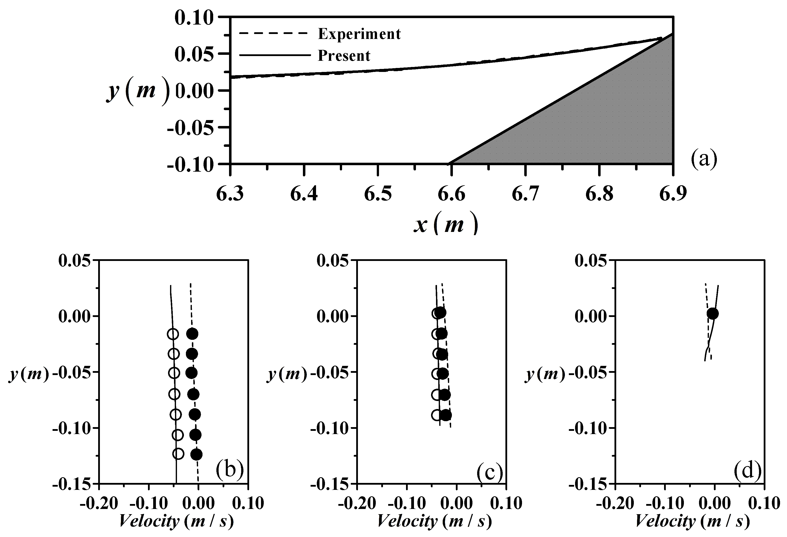
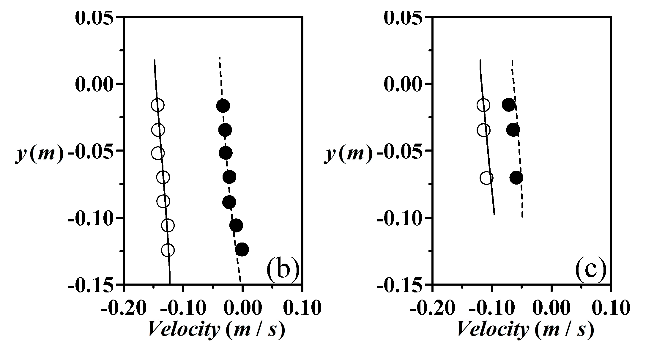
• Compared with the laboratory experimental data of free surface elevations and velocity profiles, it is demonstrated that the numerical model successfully reproduces the various stages of the solitary wave run-up and run-down on a steep seawall.
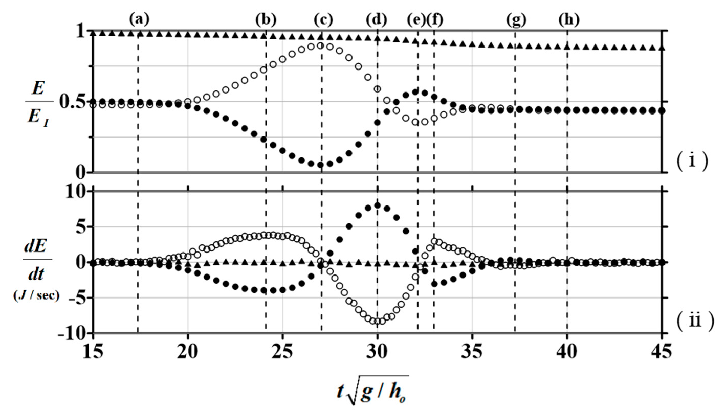
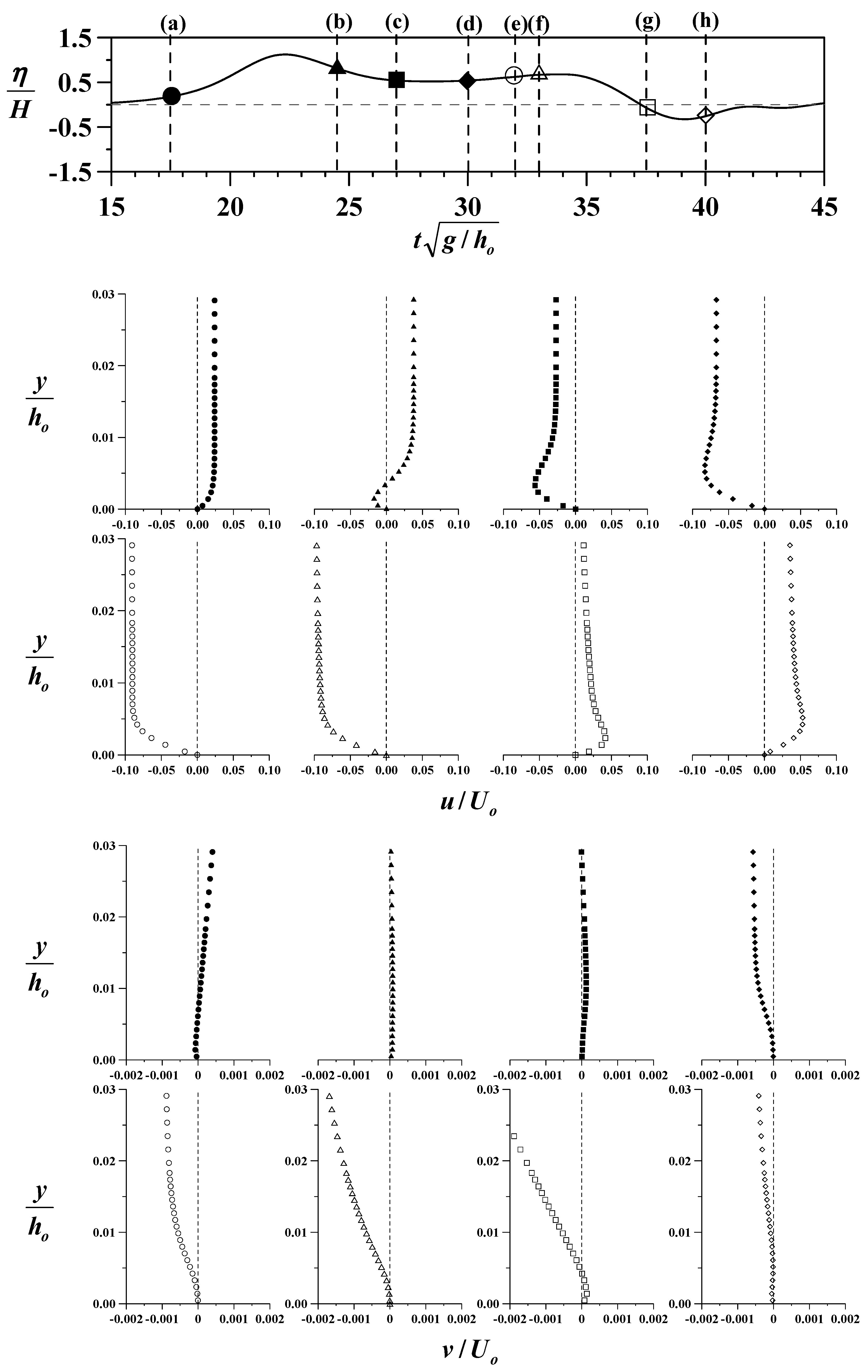
• The free surface variations during the process of a non-breaking solitary wave entering and leaving a slope at various stages are shown, as well as energy and rate of energy change over time. It can be observed that the maximum run-up height occurs when the potential energy reaches its maximum, and then reaches minimum run-up height when the second-highest rate of change in potential energy occurs.
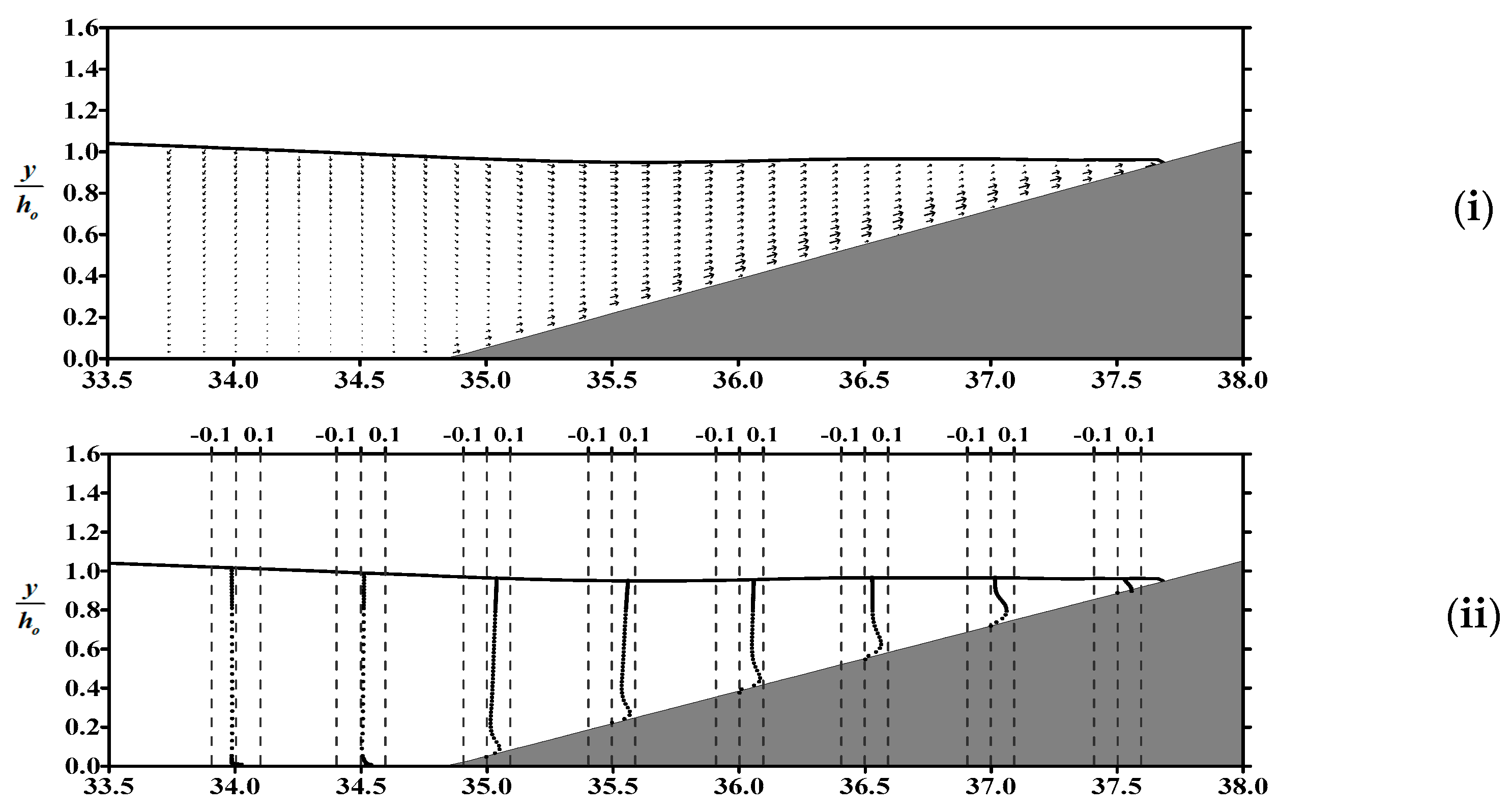
• After the arrival of the wave crest on the slope, the potential energy gradually increases and the rate of change reaches its peak. The higher velocities are concentrated at the front of the water body during the wave run-up process.
• When the leading edge of the solitary wave approaches the maximum run-up height, most of the kinetic energy in the wave has been converted into potential energy required for run-up, and most velocities approach zero, resulting in minimum kinetic energy.
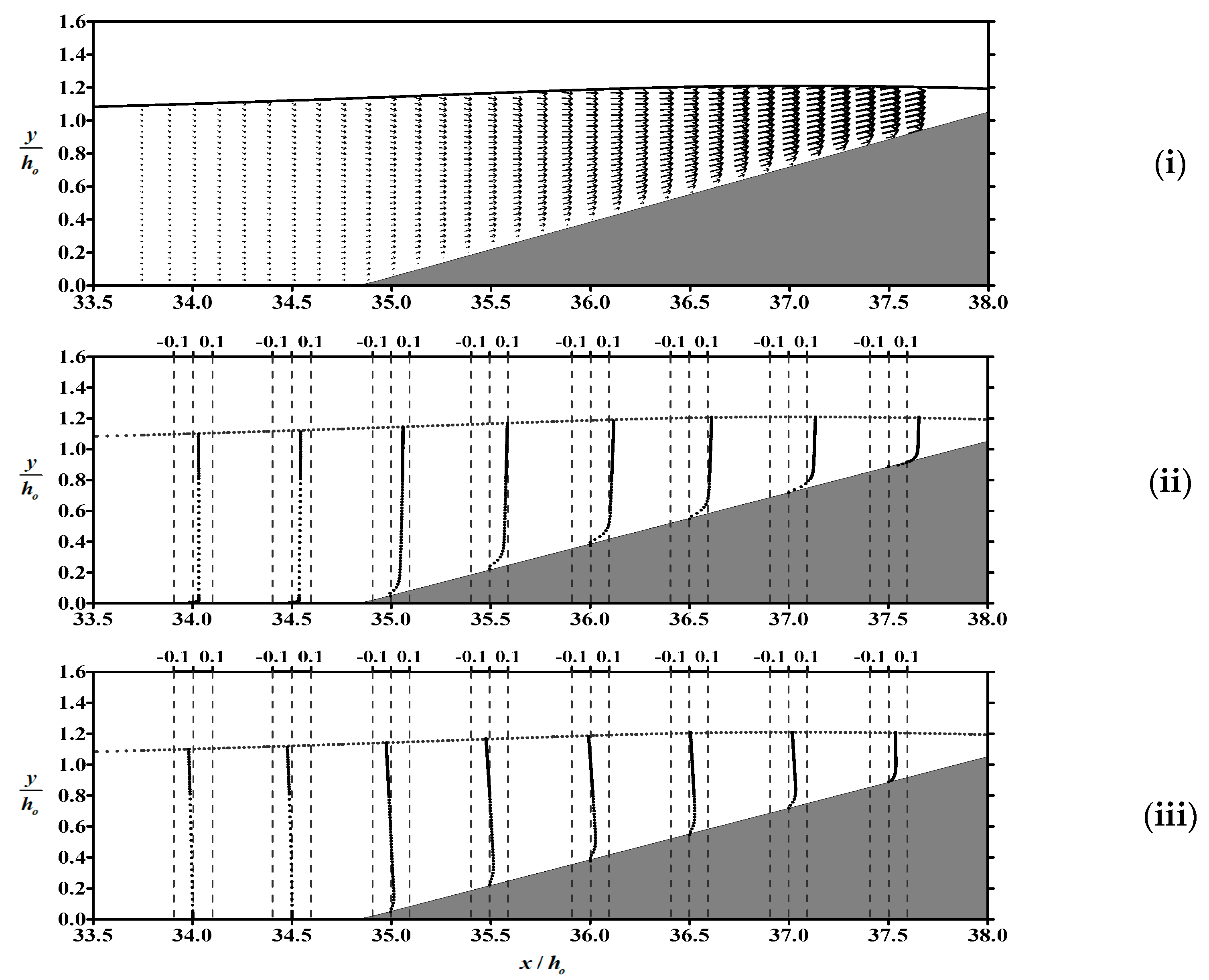
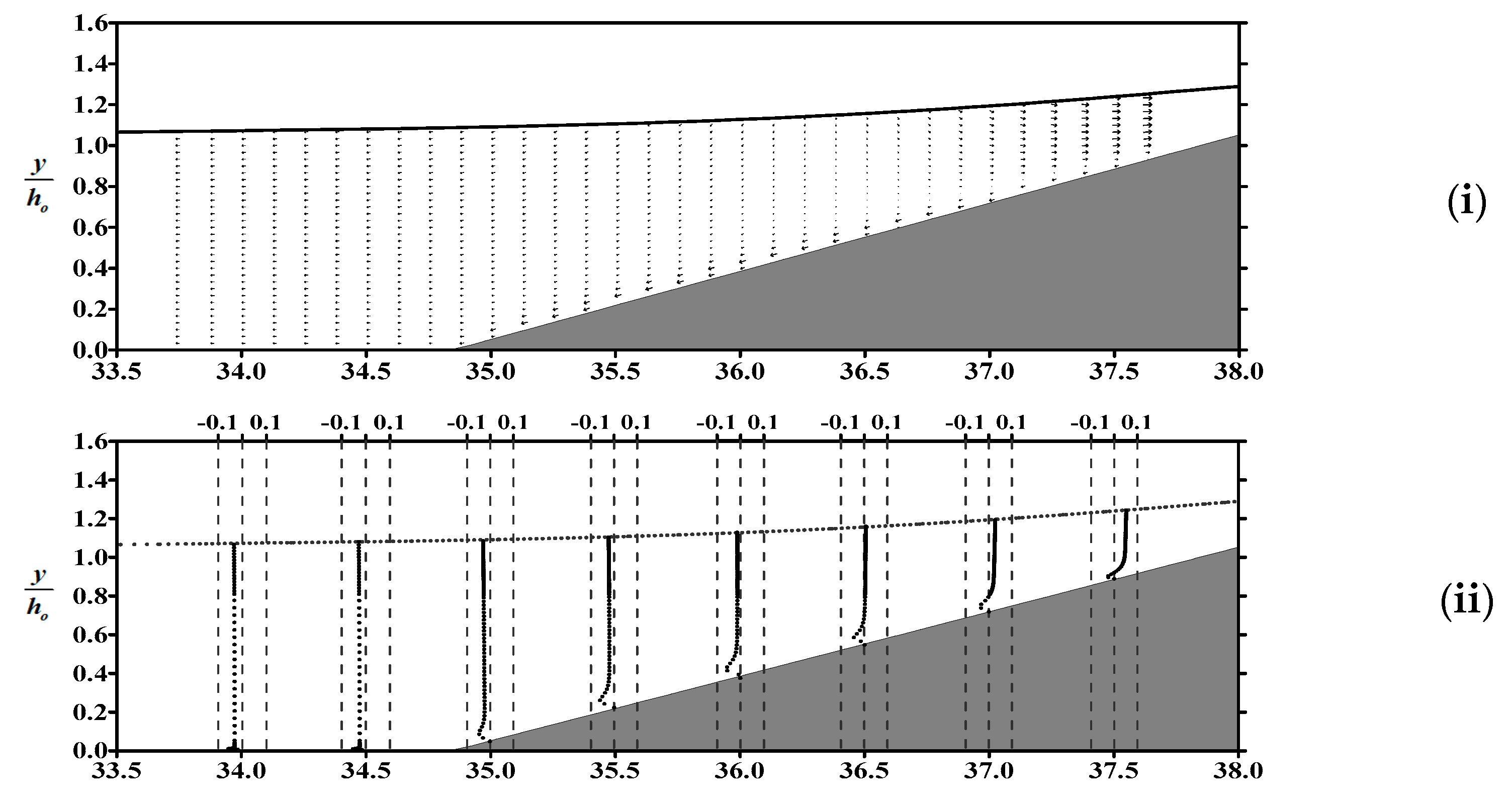
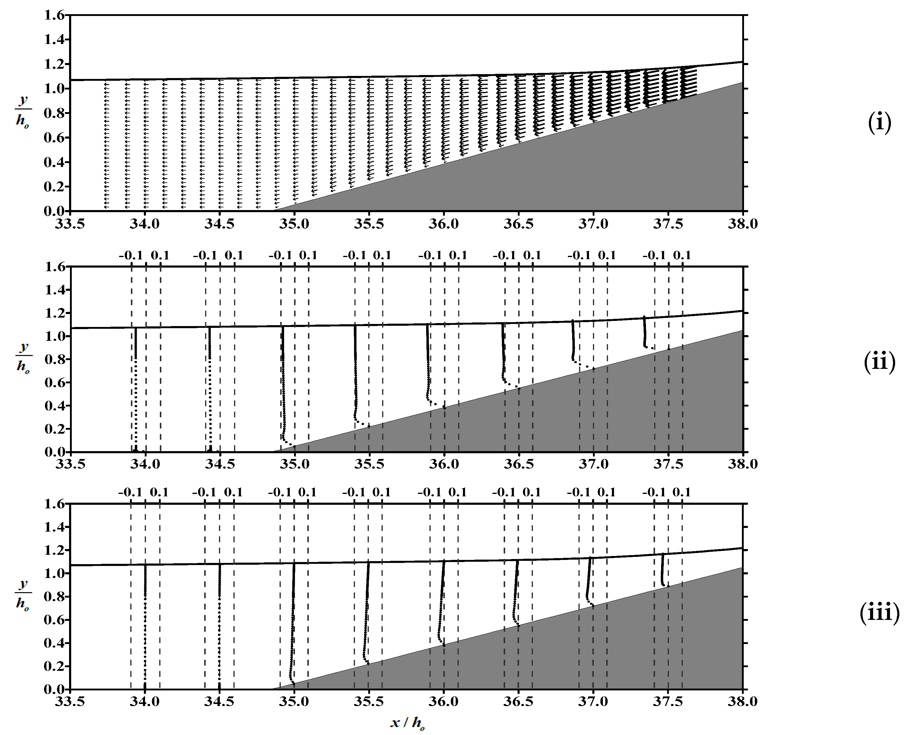
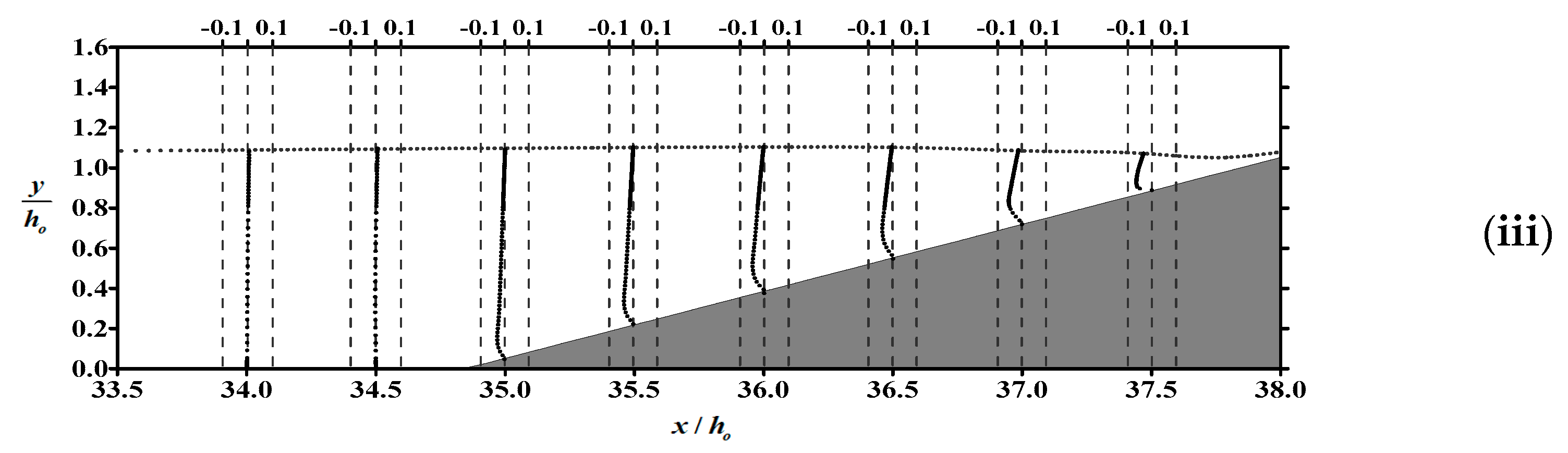
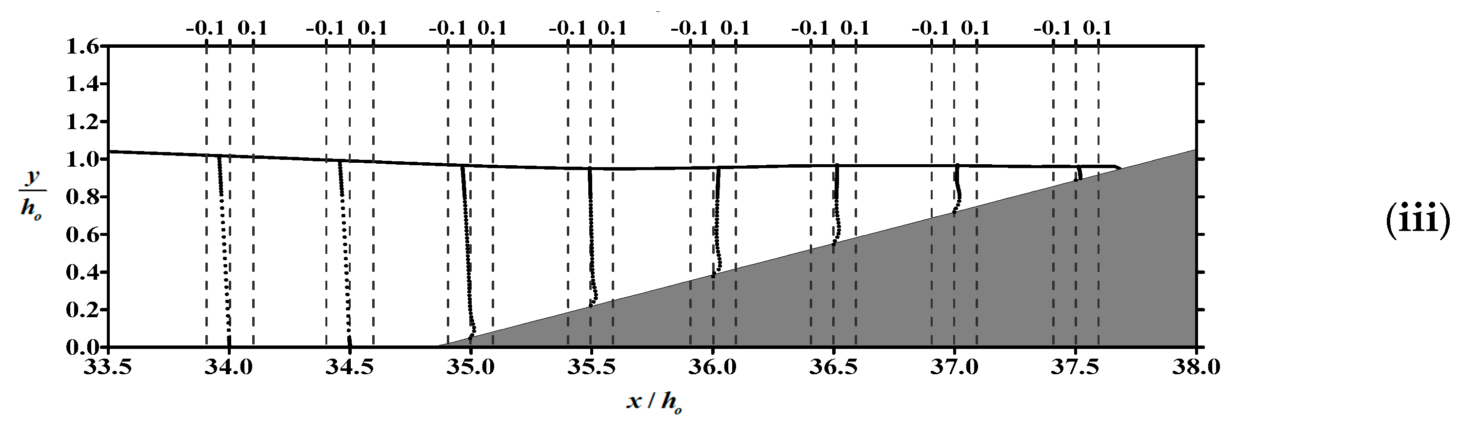
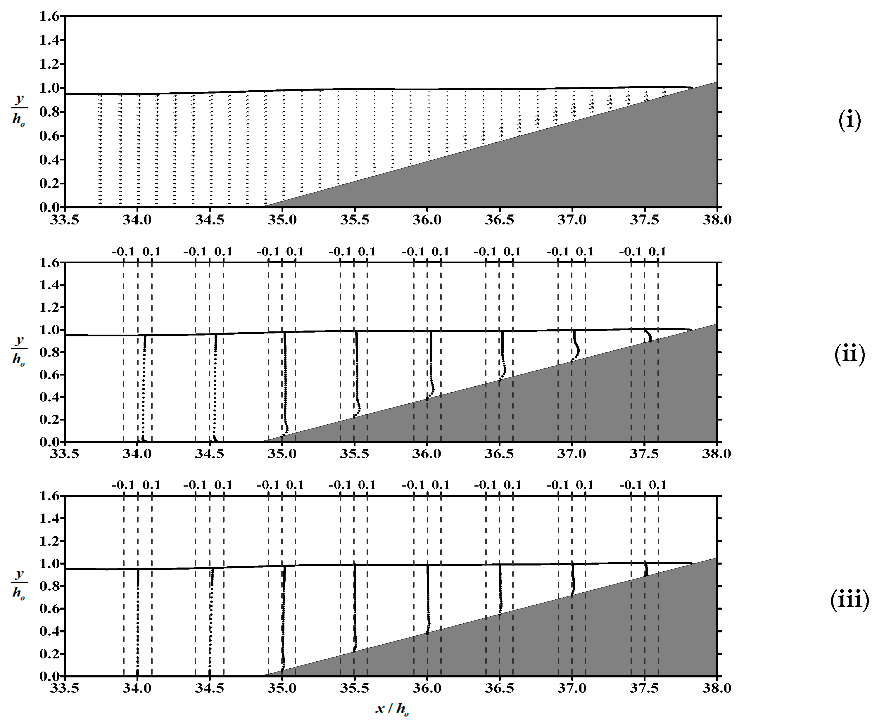
• During the run-down process, the potential energy of the solitary wave is converted into kinetic energy, redirecting the velocity of the water front in the seaward direction. The maximum flow velocity was approximately 0.304 $U_o$, occurring at $x/h_o=$ 37.5 as $t\sqrt{g/h_o}$ = 32. The flow field indicates that the highest velocity on the slope was not near the free surface but close to the sloping bed. When the water body returns to its static position, the kinetic energy and potential energy of the solitary wave tend to equalize, with approximately 10–20% of the total energy being dissipated.
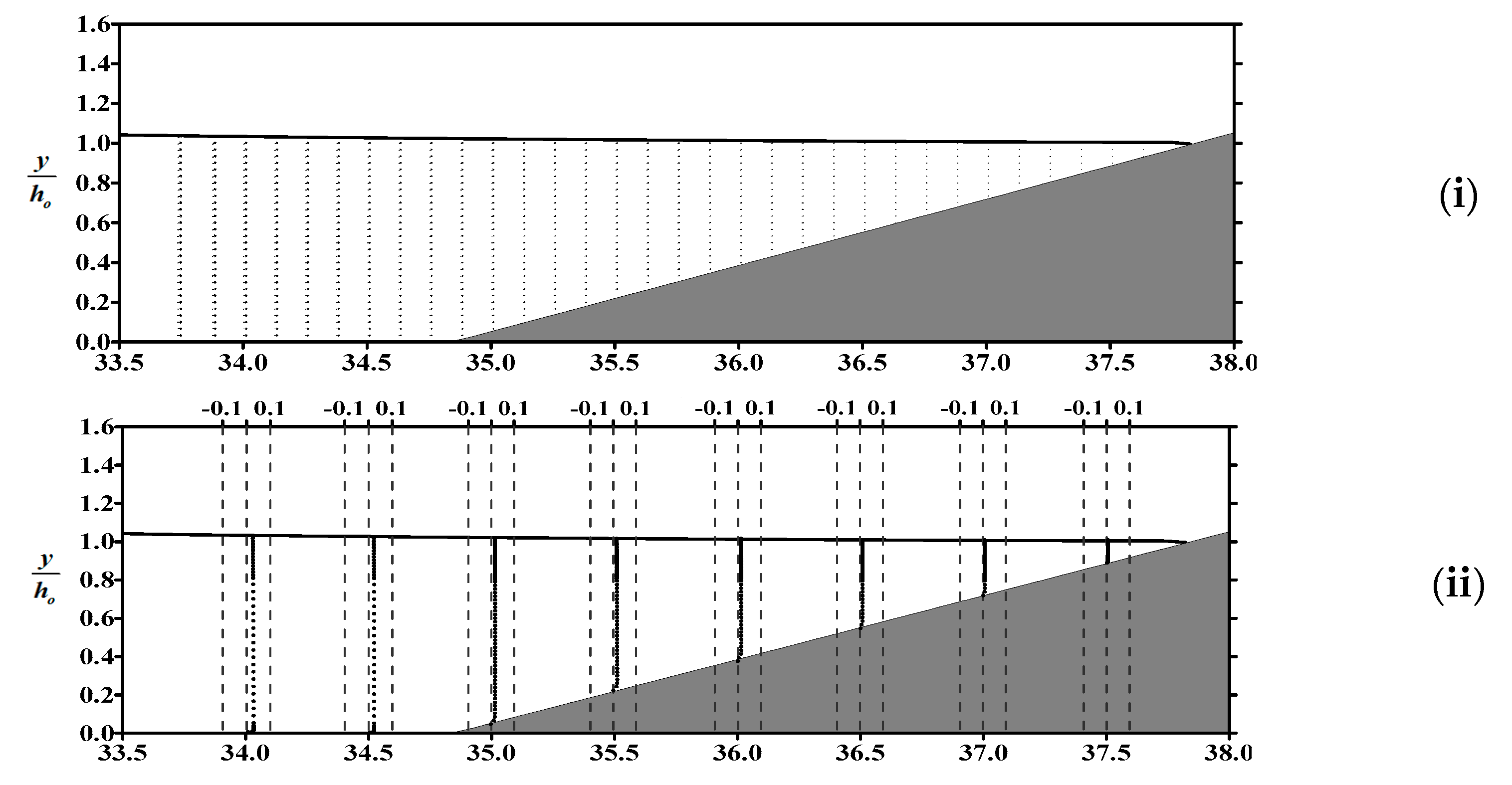
• Within the boundary layer of the flat bottom in front of the slope, the boundary layer flow is dominated by horizontal velocity. The phenomenon of reverse flow occurs in the flow field, as well as on the slope, and the gradient of velocity profile in the boundary layer near the flat bottom is significantly greater than that over the slope.
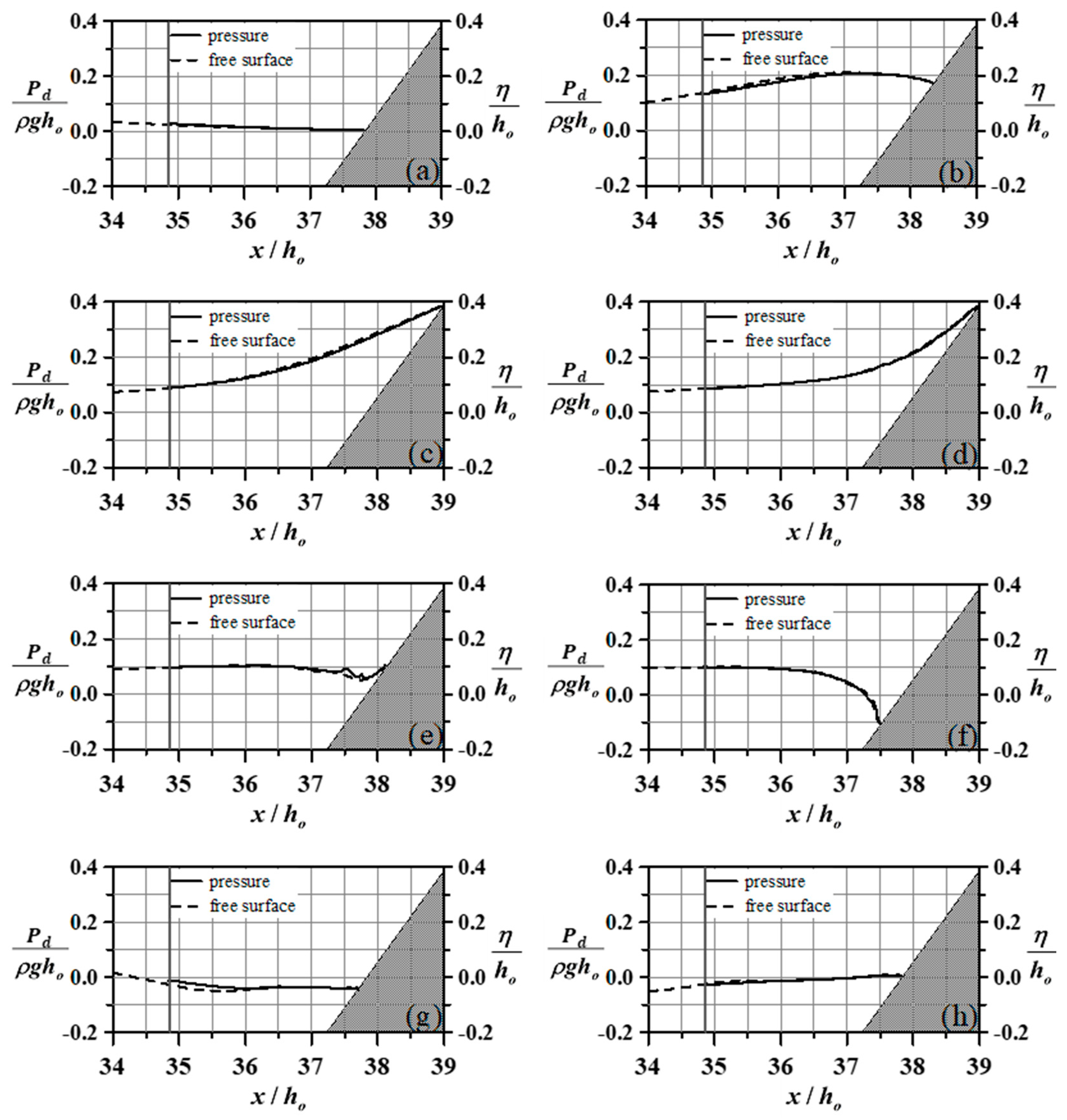
• The dynamic pressure on the sloping bed is proportional to the free surface elevation. Due to the dominant influence of the dynamic pressure gradient on the flow field in the vicinity of the bed, we can indirectly ascertain the occurrence time of undertow by examining the spatial variations in water level.

Wave breaking is often accompanied by a significant dissipation of energy, making it an important issue in seawall design. Different conditions of solitary waves and seawall slopes often lead to more complex flow patterns, breaking waves, and energy variations, which provide potential research directions for future investigations. To explore the optimal design of slopes that can withstand waves, a more detailed comparison of different cases with varying conditions of solitary waves and slope gradients could be conducted in the next phase of this study. This will be a focus of future research to further enhance our understanding in this area.

References

1. Carrier, G.F.; Greenspan, H.P. Water waves of finite amplitude on a sloping beach. J. Fluid Mech. 1958, 4, 97–109. [Google Scholar] [CrossRef]
2. Johnson, R.S.; King, R.A. Nonlinear Waves in Fluids: Finite-Amplitude Waves, Instability and Turbulence; Springer: Berlin/Heidelberg, Germany, 1983. [Google Scholar]
3. Wazwaz, A.M. Partial Differential Equations and Solitary Waves Theory; Higher Education Press and Springer: Berlin/Heidelberg, Germany, 2009. [Google Scholar]
4. Hall, J.; Watts, J. Laboratory Investigation of the Vertical Rise of Solitary Waves on Impermeable Slopes; Beach Erosion Board, US Army Corps of Engineer, Tech. Memo: Washington, DC, USA, 1953; Volume 33, p. 14. [Google Scholar]
5. Zelt, J. The run-up of nonbreaking and breaking solitary waves. Coast. Eng. 1991, 15, 205–246. [Google Scholar] [CrossRef]
6. Li, Y.; Raichlen, F. Solitary Wave Runup on Plane Slopes. J. Waterw. Port Coast. Ocean Eng. 2001, 127, 33–44. [Google Scholar] [CrossRef]
7. Shuto, N. Standing Waves in Front of a Sloping Dike. Coast. Eng. Jpn. 1972, 15, 13–23. [Google Scholar] [CrossRef]
8. Goto, C.; Shuto, N. Numerical simulation of tsunami run-up. Coast. Eng. Jpn. 1978, 21, 13–20. [Google Scholar]
9. Goto, C.; Shuto, N. Run-up of tsunamis by linear and nonlinear theories. In Proceedings of the 17th International Conference on Coastal Engineering, JSCE, Sydney, Australia, 23–28 March 1980; pp. 56–60. [Google Scholar]
10. Kim, S.K.; Liu, P.L.-F.; Liggett, J.A. Boundary integral equation solutions for solitary wave generation, propagation and run-up. Coast. Eng. 1983, 7, 299–317. [Google Scholar] [CrossRef]
11. Pelinovsky, E.; Mazova, R.K. Exact analytical solutions of nonlinear problems of tsunami wave run-up on slopes with different profiles. Nat. Hazards 1992, 6, 227–249. [Google Scholar] [CrossRef]
12. Carrier, G.F.; Wu, T.T.; Yeh, H. Tsunami run-up and draw-down on a plane beach. J. Fluid Mech. 2003, 475, 79–99. [Google Scholar] [CrossRef]
13. Synolakis, C.E. The runup of solitary waves. J. Fluid Mech. Digit. Arch. 1987, 185, 523–545. [Google Scholar] [CrossRef]
14. Tadepalli, S.; Synolakis, C.E. The run-up of N-waves on sloping beaches. Proc. R. Soc. A Math. Phys. Eng. Sci. 1994, 445, 99–112. [Google Scholar]
15. Kânoğlu, U.; Synolakis, C.E. Long wave runup on piecewise linear topographies. J. Fluid Mech. 1998, 374, 1–28. [Google Scholar] [CrossRef]
16. Kânoğlu, U. Nonlinear evolution and runup–rundown of long waves over a sloping beach. J. Fluid Mech. 2004, 513, 363–372. [Google Scholar] [CrossRef]
17. Matteo, A.; Brocchini, M. Maximum run-up, breaking conditions and dynamical forces in the swash zone: A boundary value approach. Coast. Eng. 2008, 55, 732–740. [Google Scholar] [CrossRef]
18. Synolakis, C.E. The Runup of Long Waves. Ph.D. Thesis, California Institute of Technology, Pasadena, CA, USA, 1986. [Google Scholar]
19. Li, Y.; Raichlen, F. Energy Balance Model for Breaking Solitary Wave Runup. J. Waterw. Port Coast. Ocean Eng. 2003, 129, 47–59. [Google Scholar] [CrossRef]
20. Lin, P.; Chang, K.-A.; Liu, P.L.-F. Runup and Rundown of Solitary Waves on Sloping Beaches. J. Waterw. Port Coast. Ocean Eng. 1999, 125, 247–255. [Google Scholar] [CrossRef]
21. Jensen, A.; Pedersen, G.K.; Wood, D.J. An experimental study of wave run-up at a steep beach. J. Fluid Mech. 2003, 486, 161–188. [Google Scholar] [CrossRef] [Green Version]
22. Yeh, H.H. Tsunami bore runup. Nat. Hazards 1991, 4, 209–220. [Google Scholar] [CrossRef]
23. Lin, C.; Wong, W.-Y.; Raikar, R.V.; Hwung, H.-H.; Tsai, C.-P. Characteristics of Accelerations and Pressure Gradient during Run-Down of Solitary Wave over Very Steep Beach: A Case Study. Water 2019, 11, 523. [Google Scholar] [CrossRef] [Green Version]
24. Hibberd, S.; Peregrine, D.H. Surf and run-up on a beach: A uniform bore. J. Fluid Mech. 1979, 95, 323–345. [Google Scholar] [CrossRef]
25. Kobayashi, N.; Karjadi, E.A. Surf-similarity parameter for breaking solitary-wave runup. J. Waterw. Port Coast. Ocean. Eng. 1994, 120, 645–650. [Google Scholar] [CrossRef]
26. Titov, V.V.; Synolakis, C.E. Modeling of Breaking and Nonbreaking Long-Wave Evolution and Runup Using VTCS-2. J. Waterw. Port Coast. Ocean Eng. 1995, 121, 308–316. [Google Scholar] [CrossRef]
27. Titov, V.V.; Synolakis, C.E. Numerical Modeling of Tidal Wave Runup. J. Waterw. Port Coast. Ocean Eng. 1998, 124, 157–171. [Google Scholar] [CrossRef]
28. Li, Y.; Raichlen, F. Non-breaking and breaking solitary wave run-up. J. Fluid Mech. 2002, 456, 295–318. [Google Scholar] [CrossRef] [Green Version]
29. Hubbard, M.E.; Dodd, N. A 2D numerical model of wave run-up and overtopping. Coast. Eng. 2002, 47, 1–26. [Google Scholar] [CrossRef]
30. Peregrine, D.H. Long waves on a beach. J. Fluid Mech. 1967, 27, 815–827. [Google Scholar] [CrossRef]
31. Nwogu, O. Alternative Form of Boussinesq Equations for Nearshore Wave Propagation. J. Waterw. Port Coast. Ocean Eng. 1993, 119, 618–638. [Google Scholar] [CrossRef] [Green Version]
32. Lynett, P.J.; Wu, T.-R.; Liu, P.L.-F. Modeling wave runup with depth-integrated equations. Coast. Eng. 2002, 46, 89–107. [Google Scholar] [CrossRef]
33. Avgeris, I.; Karambas, T.; Prinos, P. Boussinesq modeling of wave run-up and overtopping. In Proceedings of the 7th International Conference on HydroScience and Engineering, Philadelphia, PA, USA, 10–13 September 2006. [Google Scholar]
34. Korycansky, D.G.; Lynett, P.J. Run-up from impact tsunami. Geophys. J. Int. 2007, 170, 1076–1088. [Google Scholar] [CrossRef] [Green Version]
35. Fuhrman, D.R.; Madsen, P.A. Tsunami generation, propagation, and run-up with a high-order Boussinesq model. Coast. Eng. 2009, 56, 747–758. [Google Scholar] [CrossRef]
36. Lin, P.; Liu, P.L.-F. A numerical study of breaking waves in the surf zone. J. Fluid Mech. 1998, 359, 239–264. [Google Scholar] [CrossRef]
37. Lin, P.; Liu, P. Turbulence transport, vorticity dynamics, and solute mixing under plunging breaking waves in surf zone. J. Geophys. Res. Oceans 1998, 103, 15677–15694. [Google Scholar] [CrossRef]
38. Wood, D.J.; Pedersen, G.K.; Jensen, A. Modelling of run up of steep non-breaking waves. Ocean Eng. 2003, 30, 625–644. [Google Scholar] [CrossRef]
39. Hieu, P.D.; Tanimoto, K. Verification of a VOF-based two-phase flow model for wave breaking and wave–structure interactions. Ocean Eng. 2006, 33, 1565–1588. [Google Scholar] [CrossRef]
40. Dong, Z.; Zhan, J.-M. Numerical Modeling of Wave Evolution and Runup in Shallow Water. J. Hydrodyn. 2009, 21, 731–738. [Google Scholar] [CrossRef]
41. Huang, C.-J.; Lin, Y.-T.; Lin, C.-Y. Viscous Flow Fields Induced by a Breaking Solitary Wave over a Shelf. J. Mar. Sci. Technol. 2015, 23, 855–863. [Google Scholar]
42. Lin, C.-Y.; Huang, C.-J.; Hsu, T.-W. Viscous Flow Fields Induced by the Run-Up of Periodic Waves on Vertical and Sloping Seawalls. J. Mar. Sci. Eng. 2022, 10, 1512. [Google Scholar] [CrossRef]
43. Chen, C.-J.; Chen, H.-C. Finite analytic numerical method for unsteady two-dimensional Navier-Stokes equations. J. Comput. Phys. 1984, 53, 209–226. [Google Scholar] [CrossRef]
44. Grimshaw, R. The solitary wave in water of variable depth. J. Fluid Mech. 1970, 42, 639–656. [Google Scholar] [CrossRef]
45. Bagherizadeh, E.; Zhang, Z.; Farhadzadeh, A.; Angelidis, D.; Ghazian Arabi, M.; Moghimi, S.; Khosronejad, A. Numerical modelling of solitary wave and structure interactions using level-set and immersed boundary methods by adopting adequate inlet boundary conditions. J. Hydraul. Res. 2021, 59, 559–585. [Google Scholar] [CrossRef]
46. Enright, D.; Fedkiw, R.; Ferziger, J.; Mitchell, I. A Hybrid Particle Level Set Method for Improved Interface Capturing. J. Comput. Phys. 2002, 183, 83–116. [Google Scholar] [CrossRef] [Green Version]
47. Osher, S.; Sethian, J.A. Fronts propagating with curvature-dependent speed: Algorithms based on Hamilton-Jacobi formulations. J. Comput. Phys. 1988, 79, 12–49. [Google Scholar] [CrossRef] [Green Version]
48. Jiang, G.-S.; Shu, C.-W. Efficient Implementation of Weighted ENO Schemes. J. Comput. Phys. 1996, 126, 202–228. [Google Scholar] [CrossRef] [Green Version]
49. Peng, D.; Merriman, B.; Osher, S.; Zhao, H.; Kang, M. A PDE-Based fast local level set method. J. Comput. Phys. 1999, 155, 410–438. [Google Scholar] [CrossRef] [Green Version]
50. Huang, C.-J.; Lin, C.-Y.; Chen, C.-H. Numerical simulations of fluid-structure interaction based on Cartesian grids with two boundary velocities. Int. J. Numer. Methods Fluids 2015, 79, 138–161. [Google Scholar] [CrossRef]
51. Goring, D.G. Tsunami: The Propagation of Long Waves onto a Shelf; Technical Report No. KH-R-38; W. M. Keck Laboratory of Hydraulics and Water Resources, California Institute of Technology: Pasadena, CA, USA, 1978. [Google Scholar]
Figure 1. Comparison between numerical results of the present model and experimental data at t = 6.58 s. (a) Variation of free surface elevation, where the solid line (—) represents the numerical results of the present model and the dashed line (--) represents the experimental data of [20]. Subfigures (bd) depict velocity profiles at x = 6.397 m, x = 6.556 m, and x = 6.715 m, respectively. The solid line (—) and the dashed line (--) represent the horizontal and vertical velocities from the numerical simulations, while the symbols (○) and (●) represent horizontal and vertical velocities of the experimental data, respectively.
Water 15 02412 g001
Figure 2. Comparisons between numerical results of the present model and experimental data at t = 7.18 s. (a) Variation of free surface elevation, where the solid line (—) represents the numerical results of the present model and the dashed line (--) represents the experimental data of [20]. Subfigures (b,c) depict velocity profiles at x = 6.397 m and x = 6.556 m, respectively. The solid line (—) and the dashed line (--) represent the horizontal and vertical velocities from the numerical simulations, while the symbols (○) and (●) represent horizontal and vertical velocities of the experimental data, respectively.
Water 15 02412 g002aWater 15 02412 g002b
Figure 3. The wave profile of a solitary wave on a steep seawall at different time instants. The dimensionless times ( t g / h o ) for (ah) are 17.5, 24.5, 27, 30, 32, 33, 37.5, and 40, respectively.
Water 15 02412 g003
Figure 4. (i) The variations in energy and (ii) the rate of energy change over time during the progression of a solitary wave on a steep seawall. E I represents the total energy ( E t ) at the initial stage, and the symbols ○, ●, and ▲ represent potential energy, kinetic energy, and total energy, respectively. The dimensionless times ( t g / h o ) for (ah) are 17.5, 24.5, 27, 30, 32, 33, 37.5, and 40, respectively.
Water 15 02412 g004
Figure 5. Schematic diagram of flow distribution at t g / h o = 17.5 : (i) velocity vector field, (ii) horizontal velocity profile ( u / U o ), (iii) vertical velocity profile ( v / U o ).
Water 15 02412 g005aWater 15 02412 g005b
Figure 6. Schematic diagram of flow distribution at t g / h o = 24.5 : (i) velocity vector field, (ii) horizontal velocity profile ( u / U o ), (iii) vertical velocity profile ( v / U o ).
Water 15 02412 g006
Figure 7. Schematic diagram of flow distribution at t g / h o = 27 : (i) velocity vector field, (ii) horizontal velocity profile ( u / U o ), (iii) vertical velocity profile ( v / U o ).
Water 15 02412 g007aWater 15 02412 g007b
Figure 8. Schematic diagram of flow distribution at t g / h o = 30 : (i) velocity vector field, (ii) horizontal velocity profile ( u / U o ), (iii) vertical velocity profile ( v / U o ).
Water 15 02412 g008
Figure 9. Schematic diagram of flow distribution at t g / h o = 32 : (i) velocity vector field, (ii) horizontal velocity profile ( u / U o ), (iii) vertical velocity profile ( v / U o ).
Water 15 02412 g009aWater 15 02412 g009b
Figure 10. Schematic diagram of flow distribution at t g / h o = 33 : (i) velocity vector field, (ii) horizontal velocity profile ( u / U o ), (iii) vertical velocity profile ( v / U o ).
Water 15 02412 g010
Figure 11. Schematic diagram of flow distribution at t g / h o = 37.5 : (i) velocity vector field, (ii) horizontal velocity profile ( u / U o ), (iii) vertical velocity profile ( v / U o ).
Water 15 02412 g011aWater 15 02412 g011b
Figure 12. Schematic diagram of flow distribution at t g / h o = 40 : (i) velocity vector field, (ii) horizontal velocity profile ( u / U o ), (iii) vertical velocity profile ( v / U o ).
Water 15 02412 g012
Figure 13. Temporal sequence of the free surface ( η / H ) of the solitary wave at x / h o = 34.5 , and its corresponding profiles of horizontal velocity ( u / U o ) and vertical velocity ( v / U o ) within the boundary layer. The dimensionless times ( t g / h o ) for (ah) are 17.5, 24.5, 27, 30, 32, 33, 37.5, and 40. Eight different symbols are used to represent the horizontal and vertical velocity profiles under various phases.
Water 15 02412 g013
Figure 14. Dynamic pressure and free surface profiles of solitary wave acting on the steep seawall. The solid line represents the dimensionless dynamic pressure, and the dashed line represents the dimensionless free surface. The dimensionless times ( t g / h o ) for (ah) are 17.5, 24.5, 27, 30, 32, 33, 37.5, and 40.
Water 15 02412 g014
Disclaimer/Publisher’s Note: The statements, opinions and data contained in all publications are solely those of the individual author(s) and contributor(s) and not of MDPI and/or the editor(s). MDPI and/or the editor(s) disclaim responsibility for any injury to people or property resulting from any ideas, methods, instructions or products referred to in the content.