Abstract
Hydrology and land surface and models (HM and LSM) are essential tools for estimating global terrestrial water storage (TWS), an important component of the global water budget for assessing the accessibility and long-term variability of water supplies. With the expansion of open-source and open-data policies, the community can now perform model TWS simulation from source codes as well as directly exploit end-user hydrologic products for water resource applications. Regardless of the model effectiveness and usability, an accuracy assessment is necessary to quantify the model’s global and regional strengths, weaknesses, and reliability. This paper compares the most recent global TWS estimates from six models, namely the PCRaster Global Water Balance (PCR-GLOBWB), Noah, Noah-Multiparameterization (Noah-MP), Catchment LSM, and Variable Infiltration Capacity (VIC), and Community Atmosphere Biosphere Land Exchange (CABLE)—the latter of which is cross validated for the first time. TWS observations from the Gravity Recovery And Climate Experiment (GRACE) and GRACE Follow-On (GRACE-FO) satellite missions between 2002 and 2021 are used to validate the model. The analyses show that Noah-MP outperforms other models in terms of global average correlations and root mean square errors. PCR-GLOBWB performance is superior in irrigated regions because of the inclusion of human intervention components in the model. CABLE, a core LSM of the Australian climate model, significantly outperforms all others in Australia. CLSM performs reasonably well, but the TWS long-term trend appears to be incorrect due to an overestimated groundwater component. Noah performs similarly (but inferiorly) to Noah-MP, most likely due to model physics sharing. VIC has the least agreement with GRACE and GRACE-FO. The evaluation also sheds some light on the role of forcing data in model performance, particularly for ready-to-use products such as GLDAS, where incorporating MERRA-2 or ERA5 data into GLDAS Noah simulations may potentially improve its TWS accuracy, which has previously been overlooked due to limited modeling capacity. Despite each model’s unique strength, the ensemble mean TWS, particularly when Noah-MP and PCR-GLOBWB are included, yields better TWS estimates than an individual model result. The findings of this study could serve as a benchmark for future model development and the data published in this paper could aid in the scientific advancement and discoveries of the hydrology community.
1. Introduction
TWS is a key element of the global water budget and is closely related to a water supply’s availability and sustainability. TWS can be defined as the total storage quantity comprising soil moisture, groundwater, snow, canopy, and surface water components, all of which are vital for assessing climate variation and water scarcity [1]. However, measuring TWS on a global scale is challenging for three reasons. First, the global ground measurement network is relatively sparse; data are sampled unevenly globally, and measurements are frequently taken in developed countries. Second, various sensors are required to measure each TWS component, but most ground stations lack these comprehensive sets of equipment. The third and most important factor is the high cost of maintaining a continuous data record, which results in significant data gaps in ground observations [2].
Hydrology and land surface and models (HM and LSM) have been essential in supplementing the limited coverage of ground measurements. Models employ complex physics to simulate the terrestrial water (and energy) cycle to estimate flux exchanges and water storage (including TWS) at desired spatiotemporal resolutions [3]. The expansion of open-source policies allows the scientific community to modify and incorporate new features into models, improving model accuracy, flexibility, and usability. The Community Atmosphere Biosphere Land Exchange (CABLE) [4], Noah-Multiparameterization (Noah-MP) [5], and PCRaster Global Water Balance (PCR-GLOBWB) [6] are examples of many advanced open-source models.
CABLE is a community model that is the foundation for the Australian Community Climate and Earth-System Simulator (ACCESS) weather model. It simulates radiation, moisture, and heat/momentum exchanges between the land surface and the atmosphere. A recent CABLE development included subgrid soil and groundwater as well as a new turbulent resistance parameterization to improve the accuracy of water storage and evapotranspiration components [7]. CABLE simulation accuracy appears reasonable globally, with a notable performance at the regional level, particularly in Australia [4]. Like CABLE, Noah-MP LSM is also maintained by a (larger) community. It is one of the core LSMs of the weather research forecasting (WRF) model. Noah-MP includes multiple land process schemes, allowing users to configure appropriate optimal model physics for specific regions and applications [5]. Specifically, Noah-MP enhances the capabilities of the base model, Noah LSM, by accommodating various physics and parameterization options, such as multiple snowpack layers, one-layer vegetation canopy, a groundwater component, and a more realistic permeable frozen soil scheme. The model is frequently updated, and the assessment of Noah-MP accuracy has always been a focus [8,9,10].
Despite the overall performance of LSMs, previous research found that TWS estimates underperformed when TWS was represented without groundwater storage (GWS) or human intervention components [11]. This behavior is most noticeable in heavily irrigated areas. Advanced hydrology models such as PCR-GLOBWB incorporate human water demands to reflect a more realistic water storage variation across urban, industrial, and agricultural domains [6]. Although this concept can potentially improve hydrologic system representation, the accuracy of TWS simulations may be influenced by the quality of human impact information used. The PCR-GLOBWB results have been previously evaluated [12], but the advantage of including anthropogenic information in a model on TWS accuracy has not been thoroughly assessed (e.g., over an irrigated domain), leaving the PCR-GLOBWB benefit relative to other models unclear.
Aside from performing model simulations in-house, which necessitates extensive computing demands and programming skills, end-user products of TWS estimates are also available from the GLDAS data [13]. GLDAS employs a number of LSMs to estimate global water and energy components in near-real time. The most recent GLDAS version 2.1 includes three LSMs: Noah, Variable Infiltration Capacity (VIC), and Catchment LSM (CLSM). Noah and VIC only offer soil moisture storage (SM), snow water equivalent (SWE), and canopy water storage (CNP), whereas CLSM also includes GWS in TWS. Despite the absence of the GWS component, previous studies have reported the remarkable performance of GLDAS-Noah in terms of temporal TWS variations in many regions [14,15].
The developer’s ultimate goal is to create the best model that provides accurate hydrologic information anywhere on Earth. Previous studies confirmed that achieving such a goal is difficult; a model’s performance was observed to be regionally dependent, and an individual model could not represent accurate TWS globally. In most environmental science applications, the ensemble mean (average) value computed from multiple model outputs can be considered to improve the overall model performance [16,17]. This also applies to hydrology, where taking variants of model simulation into account can outperform the individual model scenario [18]. However, despite the variety of available model TWS simulations, the ensemble model TWS that could result in the optimal TWS estimate has not been thoroughly investigated thus far.
The only source of large-scale TWS measurements is the Gravity Recover And Climate Experiment (GRACE) and GRACE Follow-On satellite missions [19]. Both gravity missions are twin low-Earth orbit satellites equipped with GPS positioning, accelerometers, microwave (or laser in GRACE-FO) ranging, and attitude sensors that are used to map the Earth’s gravity change every month. The gravity measurements are then converted to mass variations associated with hydrologic loadings, i.e., TWS. Because gravity variations at the monthly scale are dominated by subsurface components (e.g., rootzone soil moisture, groundwater), GRACE appears to be suitable for a broad range of hydrologic applications, particularly groundwater studies [20]. For convenience, GRACE and GRACE-FO will be referred to as GRACE in this paper.
Model estimates often offer high spatiotemporal resolutions and relatively low data latency, making them valuable for local and near real-time applications that require more detailed information than satellite observations can provide. However, to ensure the reliability of the results, it is essential to assess the accuracy of these models to determine their practical validity. In this study, the TWS estimation performance of various HM and LSM models is validated against GRACE measurements. Specifically, this study incorporates the latest developments in HM and LSM (namely CABLE, Noah-MP, and PCR-GLOBWB) in the global TWS evaluation and identifies the optimal combination of model ensembles that can yield the most accurate TWS estimates. It is acknowledged that previous comparisons have been made between GRACE and model results. This study adds to previous research in three ways. First, it conducts a cross-comparison of the most recent HM and LSM developments (i.e., CABLE, Noah-MP, PCR-GLOBWB) that have not been previously considered. Second, it delves into an in-depth analysis of a ready-to-use model, which has usually been overlooked due to limited modeling capacity. The ready-to-use model was previously utilized without providing any insights into how to improve it. Lastly, this study investigates the optimal combination of ensemble model estimates that could produce the most accurate TWS, a facet that has received little attention in previous research. The findings presented in this paper can serve as a reference point for the future development of HM and LSM TWS. At the same time, the datasets generated and made publicly available by this study can facilitate scientific progress and contribute to the advancement of the hydrology, water resources, and climate community.
2. Models and Data
This section describes the data access, data processing, and model configurations used in this study. It is worth noting that most models exclude Antarctica (i.e., latitude < 60° S) from the simulation, most likely due to the high uncertainty associated with the absence of or inaccurate glacial physics. Despite having quasi-global HM/LSM outputs, the hydrologic community recognizes global HM/LSM. This study also uses the term global, but with the caveat that TWS estimates are only evaluated within the 90° N–60° S boundary (excluding Antarctica, Figure 1). The evaluation is carried out over a 20-year period, beginning in April 2002 and ending in December 2021.
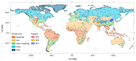
Figure 1.
Geographical locations of global river basins used in this study. The names of the basins are listed in Table S1. The Köppen-Geiger climate classification world map is used to characterize the climate zones [21]. The map also depicts heavily irrigated areas, such as the High Plains Aquifer (HPA), Northwest India (NWI), and North China Plain (NCP).
2.1. CABLE LSM
CABLE is a community LSM written in Fortran and can be accessed at https://trac.nci.org.au/trac/cable (last access: 1 October 2021). CABLE simulates radiation, moisture, and heat/momentum exchanges between the land surface and the atmosphere and can be used to estimate global TWS. Several CABLE repositories have been developed to achieve various objectives (e.g., land use change, hydrology, climate projection). CABLE SubgridSoil GroundWater (CABLE-SSGW) [4] is used in this study because of its comprehensive TWS components, particularly the inclusion of groundwater. CABLE requires precipitation, air temperature, humidity, surface pressure, wind speed, and shortwave and longwave downward radiation as forcing data. This study obtains the meteorological forcing from the Modern-Era Retrospective analysis for Research and Applications, version 2 product (MERRA-2) [22], and precipitation data from the European Centre for Medium-Range Weather Forecasts Re-Analysis product version 5 (ERA5) [23]. The substitution of precipitation is for improved model TWS estimates. All forcing variables are resampled to a 0.5° × 0.5° global grid to match the resolution of model parameters, and the model simulation is performed at 3-hourly time steps. Prior to the simulation, the model is spun up for approximately 200 years to allow the model states to reach equilibrium. This process is carried out by repeating a 2002–2021 run ten times, with the state estimates from the last time step serving as the initial states of the next spinup run. The same spinup procedure is also used for Noah-MP (Section 2.2) and PCR-GLOBWB (Section 2.3). After the simulation is completed, CABLE’s TWS is computed as the sum of soil moisture (six layers), SWE, CNP, and GWS. Then, monthly TWS estimates are calculated by averaging 3-hourly model outputs.
2.2. Noah-MP LSM
The Noah-MP was designed to incorporate a variety of model physics in order to represent an extended spectrum of terrestrial biophysical and hydrological processes [5]. The model is developed based on Noah LSM with the addition of multiple biophysical process representations, such as interactive vegetation canopy, multilayer snowpack, and dynamic groundwater, which have been shown to positively impact the estimated water cycle components [24]. The model source codes (written in Fortran) can be obtained from https://ral.ucar.edu/solutions/products/noah-multiparameterization-land-surface-model-noah-mp-lsm (last access: 1 September 2022). However, in this study, the Land Information System (LIS) [25] is used to run Noah-MP, which can speed up the process due to its parallel computation capability. The TWS components of the Noah-MP consist of soil moisture (4 layers), SWE, CNP, and GWS. This study ran the Noah-MP simulation with the default model configurations (see, e.g., https://www.jsg.utexas.edu/noah-mp/scheme-options, last access: 1 February 2023). The forcing data and simulation configuration (e.g., spatial, temporal resolution, spinup) are the same as in the CABLE case (Section 2.1).
2.3. PCR-GLOBWB HM
PCR-GLOBWB is a grid-based hydrology model that simulates continuous fields of global water balance variables such as water storage, flux, and human water consumption [6]. The model source code (written in PCRaster-Python) and hydrologic parameters can be obtained from https://github.com/UU-Hydro/PCR-GLOBWB_model (last access: 1 February 2023). Unlike the LSMs considered in this study, PCR-GLOBWB includes surface water and groundwater abstraction components. Groundwater usage is controlled by water availability and demand for irrigation, industrial sectors, and households. PCR-GLOBWB version 2.0 is used to estimate global TWS at 0.5° × 0.5° resolution. The TWS components consist of soil moisture (two layers), surface water, GWS (two layers), and SWE. The daily precipitation, air temperature, and potential evapotranspiration from the ERA5 product are used to run the model.
2.4. GLDAS
GLDAS provides comprehensive global hydrologic variables from various LSM outputs [13]. This study uses the monthly GLDAS Level 4 Version 2.1 data from the NASA Goddard Earth Sciences Data and Information Services Center (GES DISC; https://disc.gsfc.nasa.gov, last access: 1 September 2022). Outputs of three models, Noah, VIC, and CLSM, with 1° × 1° spatial resolution, are used in this study. Detailed information about the GLDAS models can be found in the accompanying product documentation. Noah-derived TWS comprises soil moisture (four layers), SWE, and CNP. The same storage components are found in VIC-derived TWS but with three soil moisture layers. CLSM’s TWS structure differs slightly from Noah and VIC in that TWS includes surface soil moisture, root zone soil moisture, SWE, CNP, and GWS.
2.5. GRACE Data
The model TWSs are evaluated using the GRACE and GRACE-FO mascon solution (RL06M.MSCNv02) of the Jet Propulsion Laboratory (JPL), California Institute of Technology, obtained from http://grace.jpl.nasa.gov (last access: 1 September 2022). The mascon with the Coastline Resolution Improvement (CRI) filter is used. The mascon approach estimates Earth’s mass variation by employing mass concentration blocks as a basis function, which improves TWS estimates when compared to a spherical harmonic solution [26]. The JPL product provides monthly TWS variations with respect to the 2004–2009 long-term mean (baseline). The product has a spatial resolution of approximately 3° × 3° and has been available since April 2002, with noticeable data gaps between July 2017 and May 2018 due to the transition between the GRACE and GRACE-FO missions.
3. Evaluation Approaches
Model TWS estimates are compared to GRACE mascon in terms of correlation, root mean square error (RMSE), long-term trend, and annual amplitude. Due to the inconsistency in spatial resolution between LSM/HM and GRACE mascon, the model TWS is resampled to mascon resolution prior to evaluation by averaging all values within a 3° × 3° mascon block. At each mascon cell, the long-term TWS mean computed from all data in the time series between April 2002 and December 2021 is subtracted from each monthly TWS data to obtain TWS variation relative to the 2002–2021 evaluation period.
3.1. Correlation and RMSE
The Pearson correlation coefficient () and RMSE are used to assess the agreement between the model and the GRACE data. At a specific mascon cell, is calculated as:
where the y vector contains the validation data (GRACE observations), the x vector contains the model estimates, is the expectation operator, and () and () are the mean and standard derivations of y and x, respectively. The RMSE is computed as:
where L denotes the length of the time series.
3.2. Long-Term Trend and Annual Amplitude
The long-term trend and annual amplitude of the time series are estimated using the least-squares fit associated with five parameters, offset (a), long-term trend (b), annual variation (c, d), and semi-annual variation (e, f). A time series () at a particular grid cell can be expressed as:
where the t vector contains time, and T denotes a one-year period. The coefficient b represents the trend, while the annual amplitude () is computed as:
Absolute trend () and amplitude differences () are used to quantify the agreement between model TWS estimates and GRACE mascon data, computed as follows:
Positive and negative values of (or ) indicate that the magnitude of model estimates is larger and smaller than GRACE, respectively. Values closer to zero represent a greater agreement between the two.
In addition, the percentage with which the estimated trend direction between models and GRACE agrees () or disagrees () can be used to evaluate their consistency in terms of long-term tendency:
where , and indicate the number of pixels where trends of both (the model and GRACE) agree (), and disagree () in direction, and is the total number of evaluated cells.
3.3. Ensemble Mean TWS
The ensemble mean TWS () can be calculated by averaging all variants of model outputs in the following manner:
where represents TWS estimates from model i and N denotes the number of models considered (1–6 in this study).
4. Results
4.1. Correlation and RMSE Evaluation
The model TWSs are compared to the GRACE mascon estimates in terms of their temporal and magnitude agreements (Figure 2). Note that areas with glaciers (e.g., Greenland, Antarctica, parts of Alaska, and South America) are excluded from the comparison to reduce model uncertainty induced by the absence or inaccurate representation of glacial physics. In all models, relatively high correlations (>0.5) are found in most parts of Europe, Australia, and South America (see Figure 2, left panel). Low or anti-correlations are observed in the Sahara Desert, Central, and high mountain Asia regions. Negative correlations are more visible in Noah and VIC, particularly over Africa and the Tibetan plateau. Considering the six models evaluated here, only Noah and VIC’s TWS simulations lack the GWS component, which could explain the poor correlations. To confirm this hypothesis, an extended analysis is performed by recalculating TWS from each model, but this time GWS is removed from CABLE, CLSM, Noah-MP, and PCR-GLOBWB, making the TWS estimates from all models relatively equivalent in terms of TWS components. However, the extended analysis’s correlation, particularly over Africa and the Tibetan plateau, does not differ significantly from the original finding. A minor effect of the missing GWS component is likely due to the fact that seasonal variation driven by soil moisture dominates the correlation, and the TWS deficiency seen in Noah and VIC could be caused by other factors, such as model configuration accuracy or forcing data. In anthropogenic areas such as Northeast China or Saudi Arabia, all models show low correlation except PCR-GLOBWB, which accounts for human water demands in the model. This reflects the advantage of incorporating the water consumption component into the TWS calculation.
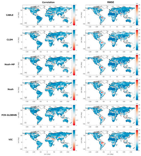
Figure 2.
Correlation coefficients (left) and RMSE (right) calculated between model TWS estimates and GRACE JPL masons (CABLE (a,b), CLSM (c,d), Noah-MP (e,f), Noah (g,h), PCR-GLOBWB (i,j), and VIC (k,l)). For ease of interpretation, a different (contrast) color scheme is used for correlation and RMSE, with cool (blue) and warm (red) colors indicating greater and lesser agreement with GRACE data, respectively.
The RMSE of all models reflects a similar spatial feature, with low RMSE observed over most of the Sahara, Southern Africa, Australia, parts of Northern China, and Russia. These areas are dominated by desert, and the low RMSE is due to a relatively small magnitude of TWS variation. High RMSE is observed in areas characterized by surface water (e.g., Amazon), anthropogenic activities (e.g., Northwest India), ice (e.g., High Mountain Asia), and earthquakes (e.g., Northern Indonesia). Notably, GRACE senses earth mass variation that includes all of the components above. In contrast, these are absent or underrepresented in most models, leading to significant mismatches in these particular regions. Due to the inclusion of surface water and water consumption components, PCR-GLOBWB has a lower RMSE than other models over Amazon, Northwest India, and North China Plain.
The global average correlation and RMSE exhibit a reasonable agreement between models and GRACE (Figure 3). The average correlation is between 0.5 and 0.6, with Noah-MP outperforming all other evaluated models. The average RMSE is about 6–9 cm, and Noah-MP has the smallest RMSE or best agreement with GRACE. However, it should be noted that Figure 3 only reflects the global average value, while the agreement at the basin level may differ. For instance, CABLE, which is primarily developed by the Australian community, provides the most accurate TWS in Australia (e.g., Murray Darling Basin, see basin 19 in Figure S1), whereas PCR-GLOBWB excels in irrigated areas (e.g., Northeast China, see, e.g., basin 22 in Figure S1).
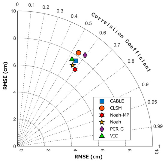
Figure 3.
Global averaged correlation coefficient (-) and RMSE (cm) values calculated between different model TWS estimates and GRACE data.
Noah-MP and Noah have similar correlations and RMSEs spatial features in several locations despite Noah-MP superiority. The resemblance is likely due to Noah-MP being built on Noah, and Noah-iMP’s physics representation contributes to improved model performance. The forcing data used in the Noah-MP model simulation also play an important role in improving TWS accuracy. Recall that Noah-MP is forced by MERRA-2 and ERA5 in this study, while Noah is forced by GLDAS forcing data. To demonstrate the impact of forcing data on model performance, the Noah-MP simulation is reperformed with GLDAS forcing data, and the correlation and RMSE are recalculated (Figure 4). Noah-MP associated with GLDAS data exhibits a similar correlation pattern to Noah, e.g., with lower correlation in Central Asia and South America (Figure 2g vs. Figure 4b), confirming the apparent role of forcing data on TWS estimates. Figure 4 also suggests that GLDAS forcing data could be the source of Noah’s negative correlation in Africa and the Tibetan plateau. Despite the use of GLDAS data, Noah-MP still outperforms Noah, which is likely attributable to the enhanced physics representation of the model. The global average correlation and RMSE both point to the same conclusion: Noah-MP (GLDAS) is closer to Noah (Figure 4c,f), and employing MERRA-2 and ERA5 forcing data improves TWS estimates.
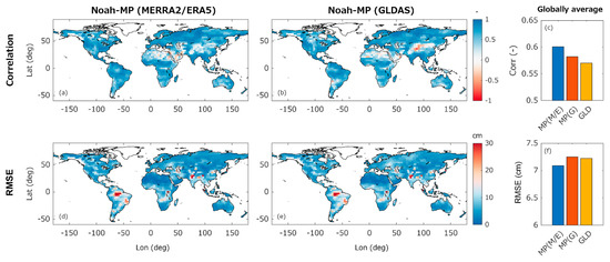
Figure 4.
Correlation coefficient (top row) and RMSE (bottom row) of Noah-MP simulations associated with forcing data from MERRA-2 and ERA-5 (M/E, left column (a,d)) and GLDAS (G, middle column (b,e)). For ease of interpretation, a different (contrast) color scheme is used for correlation and RMSE, with cool (blue) and warm (red) colors indicating greater and lesser agreement with GRACE data, respectively. The global average correlation coefficients and RMSE of two Noah-MP (MP) simulation scenarios with different forcing data, MERRA-2/ERA-5 (M/E) and GLDAS (G), are shown in the rightmost column. For reference, the global average statistical values from the Noah (GLD) simulation are also shown (c,f).
4.2. Assessing Annual Amplitude and Long-Term Trend
TWS seasonality and long-term trend are important indicators for assessing water availability, particularly when influenced by changes in climate dynamics. GRACE has been demonstrated to provide an accurate interannual TWS variation [11], which can be used to assess the model’s performance in annual amplitude and long-term trend estimates (see Equations (5) and (6)). When comparing annual amplitude between models and GRACE (Figure 5, left column), large amplitude differences are typically observed near equatorial areas, such as the Amazon, Africa, and South Asia, where TWS seasonality is relatively stronger than in higher latitude zones. GLDAS models (Figure 5c,g,k) overestimate TWS in high-latitude areas such as Europe and North America. All models exhibit underestimated annual amplitudes over the Amazon River, where surface water variation—which is missing in most models—most likely governs TWS annual variations. PCR-GLOBWB accounts for surface water storage, yielding the most accurate TWS estimate for the Amazon River (Figure 5i). PCR-GLOBWB also has the best global average agreement with GRACE, which may be attributed to the model’s more comprehensive hydrological/anthropogenic processes.
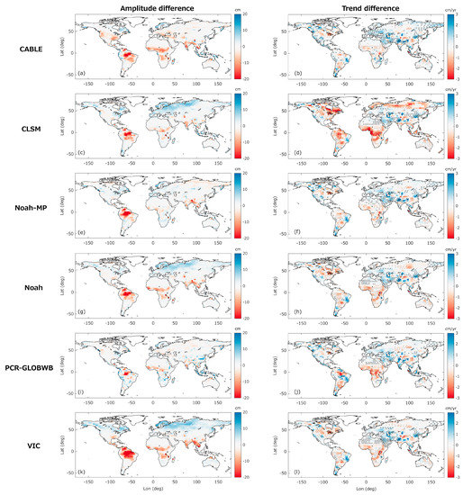
Figure 5.
The absolute annual amplitude (left column) and trend (right column) differences calculated between various model TWS results and GRACE data (CABLE (a,b), CLSM (c,d), Noah-MP (e,f), Noah (g,h), PCR-GLOBWB (i,j), and VIC (k,l)). In trend differences (right column), two different marks (cross (x) and dot (·)) are used to indicate the inconsistency in the trend estimates between models and GRACE. Cross (x) represents that model trends are positive, while GRACE shows negative trends. Conversely, dot (·) denotes that models estimate negative trends, whereas GRACE trends are positive. The locations with no marks indicate the agreement between models and GRACE trend directions. The color scheme represents the magnitude difference between models and GRACE, with cool (blue) and warm (red) color tone denoting model estimates that are larger or smaller relative to GRACE data, respectively. For instance, VIC annual amplitude difference (k) depicts a red tone over the Amazon River, indicating that VIC TWS estimates are smaller than GRACE in this area.
The spatial variability of trend differences between models and GRACE is greater than the amplitude (Figure 5, right column). The GRACE trend is higher than in models (see blue) in areas impacted by irrigation, glacial activity, and extreme events (i.e., drought, flood). These areas include the United States Great Plains, Northwest India, the North China Plain, High Mountain Asia, and Eastern Brazil, where models cannot capture the negative trend (as GRACE does) due to underrepresentation of the land processes (e.g., glacial, human water consumption), resulting in a significant trend mismatch. Additionally, models underestimate the increased trend (shown in red) over inundated areas such as the Amazon, Central Africa, and Central Asia. Surface water variation most likely dominates the trend in these areas, and models fail to capture it because such river and lake components are absent or incorrectly represented. CLSM has the greatest trend inconsistency with GRACE of any model (Figure 5d). By inspecting CLSM TWS components (Figure 6), it is discovered that the CLSM TWS trend is primarily driven by GWS, which exhibits strong negative trends (e.g., more than −2 cm/year) over areas with significant CLSM TWS trend differences.
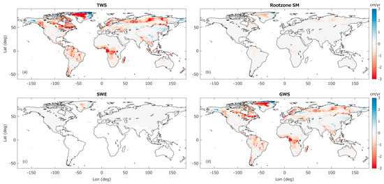
Figure 6.
Long-term trend estimates for CLSM TWS components: (a) TWS, (b) rootzone SM, (c) SWE, and (d) GWS.
Examining the agreement in trend direction (i.e., positive or negative) between models and GRACE (Equations (7) and (8)) reveals that models are able to capture the correct TWS tendency by around 50–60% globally (Table 1). For example, CABLE and GRACE observe the same direction of increased/decreased TWS by about 60% of all global mascon cells, while the remaining 40% show contrast in trend directions. GLDAS models achieve 50–55% accuracy, while CABLE, Noah-MP, and PCR-GLOBWB accuracy is about 10% higher. The best agreement with GRACE is achieved by PCR-GLOBWB and Noah-MP (62–63%), indicating that the cutting-edge model can accurately capture the correct trend direction. However, despite the distinguishable model performance, this analysis highlights the difficulty in obtaining accurate long-term trend estimates from models and the importance of future model development to improve model accuracy for such an application.

Table 1.
The number of mascon cells (%) from different models’ long-term tendency estimates which agree and disagree with GRACE.
4.3. Model Performance in Various Climate Zones and Irrigated Areas
The model’s performance differs depending on climate zones and land surface characteristics (e.g., with irrigation practice). This section evaluates the regionally average correlation, RMSE, and trend difference computed over four different climate zones, namely equatorial, arid, warm temperate, and snow, as well as three heavily irrigated areas, namely High Plains Aquifer, Northwest India, and North China Plain (see Figure 1 for locations). Note that the average trend difference is computed as RMSE to avoid cancellation between positive and negative values.
According to the climate zones analysis (Figure 7, left column), all models perform relatively well in terms of correlation over equatorial, warm temperate, and snow areas, which is likely due to strong seasonal variation in both models and GRACE (Figure 7a). The magnitude of RMSE corresponds to the magnitude of TWS variations, with higher RMSE near the equator and lower RMSE over arid areas (Figure 7c). All models provide a similar trend difference of about 0.5 cm/yr (Figure 7e), except CLSM, which is associated with the overestimated trends discussed in Section 4.2.
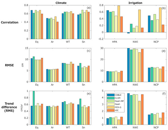
Figure 7.
Statistical values, correlation (top row (a,b)), RMSE (middle row (c,d)), and trend difference (in terms of RMS, bottom row (e,f)) calculated between various model TWS estimates and GRACE data averaged across different climate zones (left column (a,c,e)) and irrigated areas (right column (b,d,f)). Climate zones used in this analysis include equatorial (Eq), arid (Ar), warm temperate (WT), and snow (Sn), and irrigation areas include the High Plains Aquifer (HPA), Northwest India (NWI), and North China Plain (NCP). Higher correlation, lower RMSE, and lower trend difference (RMS) values indicate a stronger agreement between the model and GRACE.
Analyzing the model effectiveness in different climate conditions reveals that CABLE performs well in equatorial and arid areas but underperforms in warm temperate and snow domains (see, e.g., Figure 7a). CLSM performance is comparable to CABLE in terms of correlation and RMSE, but it is inferior in trend estimates across all climate zones (due to the overestimated GWS trends elaborated in Section 4.2). Noah-MP and PCR-GLOBWB performances are superior, ranking first or second in TWS accuracy across all metrics (i.e., highest correlation, lowest RMSE). Noah performs moderately, ranking in the middle of all models. VIC provides relatively accurate TWS amplitudes (as measured by RMSE and trend), but its temporal variability appears inconsistent with GRACE, leading to low correlation values in most climate zones.
In heavily irrigated areas, the benefit of including irrigation schemes in models is evident, with PCR-GLOBWB outperforming other models in all three metrics (Figure 7, right column). The PCR-GLOBWB correlation can reach 0.8 (i.e., in High Plains Aquifer), whereas other models (without irrigation modules) have a lower correlation, as low as −0.05 (see, e.g., CABLE in Northwest India, Figure 7b). Additional water supply or withdrawal is usually brought to farmlands, and models that rely solely on natural process representation cannot produce accurate TWS estimates. This irrigation practice alters the magnitude and timing of the TWS, resulting in the discrepancy between model estimates and GRACE. The RMSE and trend analyses show the same pattern, emphasizing the importance of including some levels of an irrigation scheme in the model to improve TWS estimates in irrigated areas.
4.4. Determining Optimal TWS Ensembles
The quality of model TWS estimates varies with location due to the fact that the accuracy of land surface physics, parameters, and forcing data is inhomogeneous in space. When the TWS simulations of different models are treated as random variables, the ensemble mean (averaged) TWS computed from several model outputs (referred to as ensemble members or realizations) may improve global TWS estimates. However, despite the potential benefit, using all available ensemble members may lead to suboptimal TWSs, given that some models produce inaccurate results. As such, identifying a set of accurate ensemble members must be performed prior to calculating the ensemble mean in order to obtain the optimal TWS estimates.
Various combinations of six ensemble members (obtained from six model TWSs) are investigated here. GRACE is used to evaluate the ensemble mean TWS in terms of correlation, RMSE, and trend difference (as RMS, see explanation in Section 3.3), and the global average values are analyzed for each combination. Figure 8 depicts the optimal statistical value from different combinations (e.g., using two (2M), three (3M), and four ensemble members (4M)) where models with color are used in that combination. For example, when only one model is used (1M), PCR-GLOBWB provides the highest correlation value, 0.66 (Figure 8a). When two models are used (2M), the ensemble mean of CABLE and PCR-GLOBWB yields the best correlation value, 0.69. The correlation values increase with the number of models and reach the highest value (0.71) when four models are used: CABLE, CLSM, Noah-MP, and PCR-GLOBWB. The values decrease when the VIC or Noah model is included in the calculation. The inclusion of PCR-GLOBWB in the ensemble mean calculation is necessary to achieve the best correlation estimate.
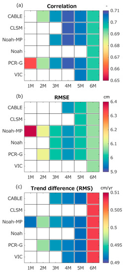
Figure 8.
Statistical results, correlation (top row (a)), RMSE (middle row (b)), and trend difference (in terms of RMS, bottom row (c)) calculated between GRACE data and various ensemble mean TWS values obtained from different model combinations. Only models with the best statistical values in the combination are displayed. For instance, when one model (1M) is used, PCR-GLOBWB (PCR-G) has the highest correlation value (see top row), and it is thus shown on the map. Similarly, when two models (2M) are analyzed, the ensemble mean of PCR-GLOBWB and CABLE yields the highest correlation value, so they are displayed. For ease of interpretation, a different (contrast) color scheme is used for different metrics, with cool (blue) and warm (red) colors indicating greater and lesser agreement with GRACE data, respectively.
For RMSE (Figure 8b), the optimal result is obtained when Noah-MP and PCR-GLOBWB are included in the combination. Similar to the correlation analysis, the ensemble mean of four models (Noah-MP, PCR-GLOBWB, Noah, and CABLE) yields the best global average RMSE, 5.9 cm. In addition, Noah-MP and PCR-GLOBWB demonstrate an advantage in trend estimation (Figure 8c). Unlike correlation and RMSE, a single ensemble member (Noah-MP) produces better trend estimates than the ensemble mean associated with two to four ensemble members. The optimal trend estimate is found when five models are used (all models except CLSM). The overestimated CLSM GWS trend contributes to the degraded trend estimate in the 6M case. This analysis sheds some light on Noah-MP and PCR-GLOBWB’s superiority in providing the best TWS estimates among all evaluated models.
5. Discussion
This study evaluates the performance of global TWS simulations from six different models. Noah-MP and PCR-GLOBWB provide the best global average TWS estimates, likely due to the comprehensive TWS components, e.g., GWS and anthropogenic influence, consistent with GRACE and GRACE-FO TWS observations. CLSM simulations, on the other hand, are not always in line with GRACE, despite the presence of GWS in the model. The thorough analysis reveals that CLSM GWS is overestimated, resulting in a significant mismatch with GRACE data. The causes of CLSM overestimated trends are beyond the scope of this study, but it is anticipated that the error might be related to an improper water distribution over surface water and snow-dominant domains, where strong GWS trends are observed. Extending model spinup times to allow groundwater stores to reach an equilibrium state may also be considered for improving CLSM TWS trend estimates.
The model performance is found to be regionally dependent. This is most likely due to the primary goal of the model, which is designed or calibrated to achieve the best performance in target regions. For instance, in Australian basins, the performance of CABLE, developed by the Commonwealth Scientific and Industrial Research Organization (Australia) is superior [4]. Similarly, the PCR-GLOBWB developed by Utrecht University (the Netherlands) performs admirably across European basins [6]. As a result, obtaining accurate global TWS from a single model is difficult. A quick solution to this issue is the use of ensemble mean TWS, which blends information from multiple models to improve overall (global) TWS accuracy. However, given that not all models produce accurate TWSs, using only the best model combination in ensemble mean calculation is critical to achieving the best results. The most important ensemble members among all six models evaluated in this study are Noah-MP and PCR-GLOBWB.
The global average RMSE obtained from this study’s model TWS simulations is about two times larger than the GRACE global average uncertainty obtained from the JPL mascon product (~3 cm). The difference between models and GRACE could be attributed to two major factors: (1) The model lacks or underrepresents some TWS components (e.g., missing GWS), and (2) GRACE contains a geophysical signal that is not associated with terrestrial water variations. For example, the analysis shows that an absent or inaccurate surface water component can cause significant RMSE over the Amazon River. Meanwhile, the RMSE evaluation near epicenter areas may be invalid due to differences in observed geophysical/hydrologic signals between models and GRACE. As such, the mismatch does not necessarily indicate poor model performance but may relate to the two’s different natures. This analysis implies the importance of incorporating hydrologic knowledge into interpreting GRACE and model simulations. Excluding areas with inconsistent geophysical/hydrologic signals from the analysis required accurate spatiotemporal geographical information, which is difficult to obtain (or is unknown). Despite this crucial challenge, separating the geophysical from hydrologic components from GRACE has already been attempted, with reasonable accuracy, albeit imperfectly and with considerable effort [27]. The global RMSE of model TWS simulation would most likely decrease if accurate signal isolations could be accomplished.
Like previous findings [11], this study encounters difficulties in using models for accurate trend estimates. The trend disagreement may be due to (but not limited to) inaccurate meteorology forcing, underrepresented model physics, or oversimplified water storage components, all of which contribute to TWS uncertainty. Some studies incorporated GRACE data into models via a data assimilation approach to improve trend estimates [28]. Despite its effectiveness, data assimilation is computationally expensive and frequently involves using a high computation performance (HPC) facility to perform ensemble model runs. Alternatively, a direct combination of GRACE and model TWS simulation can bypass model propagation and ensemble processes and requires much less computational effort [29]. The combination approach may be more suitable than data assimilation when only improved TWS (or TWS components) are of interest.
6. Conclusions
The evaluation of global TWS simulations from six models (CABLE, CLSM, Noah-MP, Noah, PCR-GLOBWB, and VIC) benchmark their performances and reveals some plausible solutions for improvement. While each model has advantages in different regions, Noah-MP and PCR-GLOBWB have the best global average correlation, RMSE, and trend estimates when evaluated with GRACE and GRACE-FO data. In the irrigated region, PCR-GLOBWB outperforms other models, demonstrating the benefit of including a human water consumption scheme in the model. Comprehensive TWS components, such as incorporating GWS into the model, could improve TWS simulation quality (observed from, e.g., Noah-MP and PCR-GLOBWB). On the other hand, the quality of TWS components is also critical, as comprehensive but inaccurate estimates lead to degraded TWS accuracy (e.g., in the CLSM case). The impact of forcing data on TWS accuracy is also evident, and the analysis suggests that MERRA-2 or ERA5 data may be used to improve the GLDAS accuracy. Furthermore, the ensemble mean TWS (computed from multiple models) could be regarded as a quick solution for improving the overall accuracy of the global TWS. However, given that not all model TWSs are accurate, it is recommended that a specific set of ensemble members must be identified to avoid achieving suboptimal TWS. The optimal TWS results are obtained by incorporating Noah-MP and PCR-GLOBWB into the ensemble mean calculation. Nevertheless, it is worth noting that PCR-GLOBWB and Noah-MP are optimal among the six evaluated models available to this study, and future research is encouraged to expand a range of models (and model configurations) to determine other possible optimal TWS or ensemble TWS estimates [12] and provide the best hydrologic information (or publicly accessible data) to the hydrology community.
Supplementary Materials
The following supporting information can be downloaded at: https://www.mdpi.com/article/10.3390/w15132456/s1, Figure S1: Correlation coefficients calculated over different river basins between various model TWS estimates and GRACE data; Table S1: The Names of the global river basins used in this study.
Funding
This research is supported by the Asian Institute of Technology (AIT) Research Initiation Grant (RIG) number SET-2023-006.
Data Availability Statement
All data used in this study are publicly available, and instructions to access the data are given in Section 2. GLDAS can be obtained from GES DISC; https://disc.gsfc.nasa.gov (last access: 1 September 2022). Due to limited computational and storage capacity, TWS estimates from CABLE, Noah-MP, and PCR-GLOBWB generated by this study are available for download upon request.
Acknowledgments
This research is supported by the Asian Institute of Technology (AIT) Research Initiation Grant (RIG) number SET-2023-006. The National Science and Technology Development Agency (NSTDA) Thailand Supercomputer Center (ThaiSC) provides computational resources under the pre-5045 and lt200041 projects.
Conflicts of Interest
The author declares no conflict of interest.
References
- Pokhrel, Y.; Felfelani, F.; Satoh, Y.; Boulange, J.; Burek, P.; Gädeke, A.; Gerten, D.; Gosling, S.N.; Grillakis, M.; Gudmundsson, L.; et al. Global Terrestrial Water Storage and Drought Severity under Climate Change. Nat. Clim. Chang. 2021, 11, 226–233. [Google Scholar] [CrossRef]
- Dorigo, W.A.; Wagner, W.; Hohensinn, R.; Hahn, S.; Paulik, C.; Xaver, A.; Gruber, A.; Drusch, M.; Mecklenburg, S.; van Oevelen, P.; et al. The International Soil Moisture Network: A Data Hosting Facility for Global in Situ Soil Moisture Measurements. Hydrol. Earth Syst. Sci. 2011, 15, 1675–1698. [Google Scholar] [CrossRef]
- Wood, E.F.; Roundy, J.K.; Troy, T.J.; van Beek, L.P.H.; Bierkens, M.F.P.; Blyth, E.; de Roo, A.; Döll, P.; Ek, M.; Famiglietti, J.; et al. Hyperresolution Global Land Surface Modeling: Meeting a Grand Challenge for Monitoring Earth’s Terrestrial Water. Water Resour. Res. 2011, 47, W05301. [Google Scholar] [CrossRef]
- Decker, M. Development and Evaluation of a New Soil Moisture and Runoff Parameterization for the CABLE LSM Including Subgrid-Scale Processes. J. Adv. Model. Earth Syst. 2015, 7, 1788–1809. [Google Scholar] [CrossRef]
- Niu, G.-Y.; Yang, Z.-L.; Mitchell, K.E.; Chen, F.; Ek, M.B.; Barlage, M.; Kumar, A.; Manning, K.; Niyogi, D.; Rosero, E.; et al. The Community Noah Land Surface Model with Multiparameterization Options (Noah-MP): 1. Model Description and Evaluation with Local-Scale Measurements. J. Geophys. Res. Atmos. 2011, 116, D12109. [Google Scholar] [CrossRef]
- Sutanudjaja, E.H.; van Beek, R.; Wanders, N.; Wada, Y.; Bosmans, J.H.C.; Drost, N.; van der Ent, R.J.; de Graaf, I.E.M.; Hoch, J.M.; de Jong, K.; et al. PCR-GLOBWB 2: A 5 arcmin Global Hydrological and Water Resources Model. Geosci. Model Dev. 2018, 11, 2429–2453. [Google Scholar] [CrossRef]
- Decker, M.; Or, D.; Pitman, A.; Ukkola, A. New Turbulent Resistance Parameterization for Soil Evaporation Based on a Pore-Scale Model: Impact on Surface Fluxes in CABLE. J. Adv. Model. Earth Syst. 2017, 9, 220–238. [Google Scholar] [CrossRef]
- Yang, Z.-L.; Niu, G.-Y.; Mitchell, K.E.; Chen, F.; Ek, M.B.; Barlage, M.; Longuevergne, L.; Manning, K.; Niyogi, D.; Tewari, M.; et al. The Community Noah Land Surface Model with Multiparameterization Options (Noah-MP): 2. Evaluation over Global River Basins. J. Geophys. Res. Atmos. 2011, 116, D12110. [Google Scholar] [CrossRef]
- Ma, N.; Niu, G.-Y.; Xia, Y.; Cai, X.; Zhang, Y.; Ma, Y.; Fang, Y. A Systematic Evaluation of Noah-MP in Simulating Land-Atmosphere Energy, Water, and Carbon Exchanges Over the Continental United States. J. Geophys. Res. Atmos. 2017, 122, 12245–12268. [Google Scholar] [CrossRef]
- Li, J.; Miao, C.; Zhang, G.; Fang, Y.-H.; Shangguan, W.; Niu, G.-Y. Global Evaluation of the Noah-MP Land Surface Model and Suggestions for Selecting Parameterization Schemes. J. Geophys. Res. Atmos. 2022, 127, e2021JD035753. [Google Scholar] [CrossRef]
- Scanlon, B.R.; Zhang, Z.; Save, H.; Sun, A.Y.; Schmied, H.M.; van Beek, L.P.H.; Wiese, D.N.; Wada, Y.; Long, D.; Reedy, R.C.; et al. Global Models Underestimate Large Decadal Declining and Rising Water Storage Trends Relative to GRACE Satellite Data. Proc. Natl. Acad. Sci. USA 2018, 115, E1080–E1089. [Google Scholar] [CrossRef] [PubMed]
- Bolaños Chavarría, S.; Werner, M.; Salazar, J.F.; Betancur Vargas, T. Benchmarking Global Hydrological and Land Surface Models against GRACE in a Medium-Sized Tropical Basin. Hydrol. Earth Syst. Sci. 2022, 26, 4323–4344. [Google Scholar] [CrossRef]
- Rodell, M.; Houser, P.R.; Jambor, U.; Gottschalck, J.; Mitchell, K.; Meng, C.-J.; Arsenault, K.; Cosgrove, B.; Radakovich, J.; Bosilovich, M.; et al. The Global Land Data Assimilation System. Bull. Am. Meteorol. Soc. 2004, 85, 381–394. [Google Scholar] [CrossRef]
- Syed, T.H.; Famiglietti, J.S.; Rodell, M.; Chen, J.; Wilson, C.R. Analysis of Terrestrial Water Storage Changes from GRACE and GLDAS. Water Resour. Res. 2008, 44, W02433. [Google Scholar] [CrossRef]
- Awange, J.L.; Forootan, E.; Kuhn, M.; Kusche, J.; Heck, B. Water Storage Changes and Climate Variability within the Nile Basin between 2002 and 2011. Adv. Water Resour. 2014, 73, 1–15. [Google Scholar] [CrossRef]
- Willcock, S.; Hooftman, D.A.P.; Blanchard, R.; Dawson, T.P.; Hickler, T.; Lindeskog, M.; Martinez-Lopez, J.; Reyers, B.; Watts, S.M.; Eigenbrod, F.; et al. Ensembles of Ecosystem Service Models Can Improve Accuracy and Indicate Uncertainty. Sci. Total Environ. 2020, 747, 141006. [Google Scholar] [CrossRef]
- Jose, D.M.; Vincent, A.M.; Dwarakish, G.S. Improving Multiple Model Ensemble Predictions of Daily Precipitation and Temperature through Machine Learning Techniques. Sci. Rep. 2022, 12, 4678. [Google Scholar] [CrossRef]
- Razavi, T.; Coulibaly, P. Improving Streamflow Estimation in Ungauged Basins Using a Multi-Modelling Approach. Hydrol. Sci. J. 2016, 61, 2668–2679. [Google Scholar] [CrossRef]
- Tapley, B.D.; Watkins, M.M.; Flechtner, F.; Reigber, C.; Bettadpur, S.; Rodell, M.; Sasgen, I.; Famiglietti, J.S.; Landerer, F.W.; Chambers, D.P.; et al. Contributions of GRACE to Understanding Climate Change. Nat. Clim. Chang. 2019, 9, 358. [Google Scholar] [CrossRef]
- Yin, W.; Li, T.; Zheng, W.; Hu, L.; Han, S.-C.; Tangdamrongsub, N.; Šprlák, M.; Huang, Z. Improving Regional Groundwater Storage Estimates from GRACE and Global Hydrological Models over Tasmania, Australia. Hydrogeol. J. 2020, 28, 1809–1825. [Google Scholar] [CrossRef]
- Kottek, M.; Grieser, J.; Beck, C.; Rudolf, B.; Rubel, F. World Map of the Köppen-Geiger Climate Classification Updated. Meteorol. Z. 2006, 15, 259–263. [Google Scholar] [CrossRef] [PubMed]
- Gelaro, R.; McCarty, W.; Suárez, M.J.; Todling, R.; Molod, A.; Takacs, L.; Randles, C.A.; Darmenov, A.; Bosilovich, M.G.; Reichle, R.; et al. The Modern-Era Retrospective Analysis for Research and Applications, Version 2 (MERRA-2). J. Clim. 2017, 30, 5419–5454. [Google Scholar] [CrossRef] [PubMed]
- Hersbach, H.; Bell, B.; Berrisford, P.; Hirahara, S.; Horányi, A.; Muñoz-Sabater, J.; Nicolas, J.; Peubey, C.; Radu, R.; Schepers, D.; et al. The ERA5 Global Reanalysis. Q. J. R. Meteorol. Soc. 2020, 146, 1999–2049. [Google Scholar] [CrossRef]
- Cai, X.; Yang, Z.-L.; David, C.H.; Niu, G.-Y.; Rodell, M. Hydrological Evaluation of the Noah-MP Land Surface Model for the Mississippi River Basin. J. Geophys. Res. Atmos. 2014, 119, 23–38. [Google Scholar] [CrossRef]
- Peters-Lidard, C.D.; Houser, P.R.; Tian, Y.; Kumar, S.V.; Geiger, J.; Olden, S.; Lighty, L.; Doty, B.; Dirmeyer, P.; Adams, J.; et al. High-Performance Earth System Modeling with NASA/GSFC’s Land Information System. Innov. Syst. Softw. Eng. 2007, 3, 157–165. [Google Scholar] [CrossRef]
- Rowlands, D.D.; Luthcke, S.B.; McCarthy, J.J.; Klosko, S.M.; Chinn, D.S.; Lemoine, F.G.; Boy, J.-P.; Sabaka, T.J. Global Mass Flux Solutions from GRACE: A Comparison of Parameter Estimation Strategies—Mass Concentrations versus Stokes Coefficients. J. Geophys. Res. Solid Earth 2010, 115, B01403. [Google Scholar] [CrossRef]
- Deggim, S.; Eicker, A.; Schawohl, L.; Gerdener, H.; Schulze, K.; Engels, O.; Kusche, J.; Saraswati, A.T.; van Dam, T.; Ellenbeck, L.; et al. RECOG RL01: Correcting GRACE Total Water Storage Estimates for Global Lakes/Reservoirs and Earthquakes. Earth Syst. Sci. Data 2021, 13, 2227–2244. [Google Scholar] [CrossRef]
- Li, B.; Rodell, M.; Kumar, S.; Beaudoing, H.K.; Getirana, A.; Zaitchik, B.F.; de Goncalves, L.G.; Cossetin, C.; Bhanja, S.; Mukherjee, A.; et al. Global GRACE Data Assimilation for Groundwater and Drought Monitoring: Advances and Challenges. Water Resour. Res. 2019, 55, 7564–7586. [Google Scholar] [CrossRef]
- Tangdamrongsub, N.; Hwang, C.; Borak, J.S.; Prabnakorn, S.; Han, J. Optimizing GRACE/GRACE-FO Data and a Priori Hydrological Knowledge for Improved Global Terrestial Water Storage Component Estimates. J. Hydrol. 2021, 598, 126463. [Google Scholar] [CrossRef]


Disclaimer/Publisher’s Note: The statements, opinions and data contained in all publications are solely those of the individual author(s) and contributor(s) and not of MDPI and/or the editor(s). MDPI and/or the editor(s) disclaim responsibility for any injury to people or property resulting from any ideas, methods, instructions or products referred to in the content. |
© 2023 by the author. Licensee MDPI, Basel, Switzerland. This article is an open access article distributed under the terms and conditions of the Creative Commons Attribution (CC BY) license (https://creativecommons.org/licenses/by/4.0/).