Article

Water Quality Prediction Based on the KF-LSTM Encoder-Decoder Network: A Case Study with Missing Data Collection

1
Department of Computer Science, Shantou University, Shantou 515063, China
2
Guangdong Province Shantou Ecological Environment Monitoring Central Station, Shantou 515057, China
*
Author to whom correspondence should be addressed.
Water 2023, 15(14), 2542; https://doi.org/10.3390/w15142542
Submission received: 28 May 2023 / Revised: 3 July 2023 / Accepted: 4 July 2023 / Published: 11 July 2023

Abstract

:
This paper focuses on water quality prediction in the presence of a large number of missing values in water quality monitoring data. Current water quality monitoring data mostly come from different monitoring stations in different water bodies. As the duration of water quality monitoring increases, the complexity of water quality data also increases, and missing data is a common and difficult to avoid problem in water quality monitoring. In order to fully exploit the valuable features of the monitored data and improve the accuracy of water quality prediction models, we propose a long short-term memory (LSTM) encoder-decoder model that combines a Kalman filter (KF) with an attention mechanism. The Kalman filter in the model can quickly complete the reconstruction and pre-processing of hydrological data. The attention mechanism is added between the decoder and the encoder to solve the problem that traditional recursive neural network models lose long-range information and fully exploit the interaction information among high-dimensional covariate data. Using original data from the Haimen Bay water quality monitoring station in the Lianjiang River Basin for analysis, we trained and tested our model using detection data from 1 January 2019 to 30 June 2020 to predict future water quality. The results show that compared with traditional LSTM models, KF-LSTM models reduce the average absolute error ( M A E ) by 10%, the mean square error ( M S E ) by 21.2%, the root mean square error ( R M S E ) by 13.2%, while increasing the coefficient of determination ( R 2 ) by 4.5%. This model is more suitable for situations where there are many missing values in water quality data, while providing new solutions for real-time management of urban aquatic environments.

1. Introduction

River pollution has profound effects on all aspects of human life. The discharge of large amounts of pollutants and domestic wastewater makes it challenging to maintain the ecological stability of rivers, which in turn directly or indirectly affects the ecological balance around them [1,2,3]. In recent years, scientists have proposed various scientifically effective methods for managing river pollutants. For example, Tayseer M. Alasri et al. proposed an effective method for photocatalytic degradation of dissolved organic dyes [4], while Mohamed Mokhtar M. Mostafa et al. proposed a method for managing solid waste from aluminium cans and effectively reducing its impact on the environment [5]. The use of machine learning methods can effectively monitor and predict changes in water quality data, which has a more beneficial impact on the livability and resilience of smart cities [6]. This includes: (1) improving the efficiency of urban water supply management and the safety of water quality to significantly improve the quality of drinking water and the living standards of urban residents; (2) improving emergency response capabilities to sudden water pollution incidents; (3) helping cities to develop more scientific and sustainable plans for the development and use of water resources to support urban economic development.
Therefore, the development of mathematical models for predicting changes in water quality plays an important role in detecting changes in water quality and pollution situations in a more timely manner, predicting future conditions, and formulating scientific responses to ensure the safety and stability of aquatic ecosystems [7].
Traditional water quality analysis methods rely heavily on a large number of manual operations, requiring the selection of monitoring points in the river to be tested and the collection of samples at regular intervals, which are then taken to the laboratory for analysis and identification. Although the traditional analysis methods can reflect the pollution situation of water quality to a certain extent, there are some shortcomings that make the traditional testing methods unable to achieve timely detection of water pollution and difficult to prevent enterprises from discharging industrial wastewater exceeding the standard into the river, for example, the testing process requires a lot of human and material resources and time, the sample collection and processing process is easily disturbed, thus causing errors, the testing is also difficult to prevent enterprises from discharging industrial wastewater exceeding the standard into the river [8].
With the advent of artificial neural networks, they have become widely used in water quality prediction due to their non-linear adaptability and data processing capabilities. With the continuous development of computer hardware and computing power, the depth of neural networks continues to increase, allowing them to encode more abstract content. Among them, recurrent neural networks (RNN) have better modelling capabilities for short-term and long-term time relationships in complex data, making them more suitable for modelling water quality sequence data [9]. As the length of sequence data increases, the disappearance or explosion of gradients becomes a serious problem for RNN models. It is difficult for the model to capture the long-term features of the sequences and the prediction results are often unsatisfactory. Traditional RNN models are unable to handle high-dimensional data; high-dimensional covariate data are compressed into fixed-length vectors, resulting in loss of covariate feature information. In addition, water quality monitoring stations may be subject to various uncontrollable factors such as climatic conditions, equipment environmental changes, or battery loss, which can result in a large number of missing values in the monitoring data. The presence of many missing values can seriously affect the final prediction results by introducing statistical bias into the analysis process, leading to reduced estimation accuracy and biased prediction effects [10].
This paper proposes a model framework based on an encoder-decoder architecture to address the above issues. An LSTM model combining the Kalman filter and attention mechanism was built to predict the dissolved oxygen content in the Haimen Bay monitoring station data of the Lianjiang River in Guangdong, China. Several sets of different time series models were compared to demonstrate the effectiveness of the proposed model. The main contributions of this paper are as follows:
(1)
In this article, a Kalman filter is used to process raw data from monitoring stations, perform optimal estimation on missing values in the original data, fill in missing data, and smooth noise reduction on the original data to fully exploit all data features and improve the accuracy of model prediction.
(2)
In the traditional encoder-decoder architecture, an attention mechanism is introduced to capture long-range dependent features and multi-dimensional covariate information in sequences. This helps to overcome the shortcoming of traditional RNN models, which forget long-range data information and fully exploit interactive information from high-dimensional data.
(3)
We compare several traditional time series prediction models. The model proposed in this article performs better than other comparative models in predicting dissolved oxygen in the Lianjiang River in Guangdong, China.
This article is divided into several parts for discussion. Section 2 provides an overview of recent research on water quality prediction in both national and international contexts. Section 3 presents the overall construction of the model. Section 4 presents the results of the model, a comparison between different models and a discussion of the hyperparameters of the model. Section 5 presents the conclusions of this paper and future research directions.

2. Related Work

The current water quality prediction model is a type of time sequence prediction model, the general idea is to predict the result of water quality in the future by processing the model of water quality data collected in the past period [11]. From simple to complex machine learning model research, researchers have proposed a large number of excellent models for water quality problems, offering different modelling capabilities.

2.1. Machine Learning Methods

In machine learning, models are divided into white box, grey box and black box models according to their interpretability and transparency. Early white box models were based on simple mathematical and statistical methods, typically based on the statistical characteristics of a time series, using past time data to predict future data, building a simple method, and Siros Shahriari [12] and others used the Autoregressive Moving Average Model (ARMA) to model time series trends combined with the GARCH model to complete a model of traffic sequence that takes into account space and time. Zhiyang Zhao [13] uses the Seasonal Autoregressive Integrated Moving Average Model (SARIMA) to combine the LSTM model, build the SARIMA-LSTM model and apply it to influenza prediction, compensating for the problem of the non-linear part of the SARIMA model prediction and the poor accuracy of direct prediction of the original sequence. Hongbin Dai [14] combined with Vector Autoregression (VAR) and XGBoost to predict the ozone content in China’s atmosphere, and compared the XGboost results with a better boost.But this kind of white box model does not predict complex nonlinear, non-flat or noisy data, and is not suitable for larger and complex data sets.
The grey box model between the white box model and the black box model has better performance and interpretability, reduces the cost of modelling and improves the versatility of the model, and has a very wide range of applications in practice. Common grey box models such as support for vector regression (SVM) [15], XGBoost [16], Logical Regression [17], Random Forest [18] and so on. Given the conventional WQI methodology, which requires a lot of time and monitoring costs to calculate water quality standards, Jun Yung Ho and others [19] found that using decision tree models to analyse parameters with a smaller impact on water quality and prediction accuracy of more than 75.0% in the case of reduced parameter type input. Lu [20] and others have proposed two models of XGboost and Random Forest (RF) that improve the performance in predicting Tualatin River water quality data using adaptive noise fully integrated experience with modular noise decomposition technology.Tadesse G. Wakjira [21] proposed a new interpretable predictive model based on machine learning to interpret XGBoost model output, and built a user-friendly web prediction tool to quickly and effectively predict the horizontal circular response of back-foundation swaying steel bridges. Subhasis Giri [22] used random forest classification and return models to predict uranium concentrations in private drinking water wells in New Jersey, achieving prediction accuracies of 66% and 55%. Jianlong Xu [23] and others achieved 92.94% accuracy in predicting salinity of coastal waters based on the random forest water quality prediction framework, and successfully reproduced the salt distribution of Shenzhen Bay by remote sensing. However, the white box and grey box models in traditional machine learning have strict data requirements, and the models generated by these data are linearly constrained, and the long-term prediction effect is not stable and requires more time cost.
Traditional machine learning is gradually becoming scarce in the process of handling large amounts of congested data, while neural network-based deep learning as a black box model, through a large number of data iteration optimization to obtain the optimal weight and deviation configuration, Using the neural networks strong nonlinear adaptation ability to process time-series data, learn more profound information, with higher predictive performance and accuracy, such as back-propagation neural networks (BPNN) [24], deep belief network (DBN) [25] and so on. Sarkar and Pandey [26] studied artificial neural networks (ANN), selected self-organized mapping (SOM) and combined with the K-means algorithm, which can solve the nonlinear relationships between variables that cannot be extracted in traditional PCA analysis, and simulated the dissolved oxygen concentration in the Amuna River, but the structure of the ANN model is difficult to adjust, and the data noise sensitivity characteristics tend to make the ANN model less likely to the expected results when training water quality data. A 2017 study by Anita Csábrági [27], which used multi-set pretransmission and backtransmission neural networks to process the water quality of the Hungarian Danube in 1998–2003 and predict the DO in it, showed that the generic regression neural network GRNN and the radial-based neural system RBFNN performed better than the classical multi-layer sensor MLPNN. Yue Zhang [28] and others chose BP neural networks and Random Forest models to validate accurate predictions of flood flow for the past N hours in the current reservoir in Zhejiang Province, Shandong, taking advantage of BP neural networks to make multi-stage prediction based on reducing the complexity of the model.
With the development of machine learning and the production of large amounts of data, people began to use more sophisticated black box models, among which the common models are RNN and (volume neural network) CNN models, but traditional RNN models and CNN models in dealing with long sequence input problems, as the length of the sequence increases, will produce a marked explosion of scale and long-term information loss problems, and to mitigate such problems Sepp Hochreiter and others proposed the LSTM [29] model. LSTM models based on RNN architectures have been proposed to mitigate problems inherent in traditional RNN models, and have been widely used for predicting water quality sequences [30]. In 2019, TAO and others [31] realised air pollution prediction using a one-dimensional volume combined with a two-way door cycle unit, demonstrating the advantage of the model in comparison with machine learning. Ma et al. [32] used LSTM to eliminate the problem of reverse transmission error decline to predict the traffic flow speed of major highways in the Beijing region, proving that it is superior to other models of RNN structures in terms of accuracy and stability. Liu et al. [33] used the LSTM model to accurately predict the quality of drinking water in the Yangtze River Guayaquil, demonstrating the feasibility of LSTM as a tool for predicting water quality.
Due to the presence of data noise, nonlinear models are prone to overfitting. To effectively improve the ability of the model to handle nonlinear data, it is necessary to smooth the original data and reduce the effect of noise. Filters are an effective method for dealing with data noise and have been widely used in time series data processing in recent years, such as: Moving Average Filter (MA Filter) [34], Exponential Moving Average Filter (MM Filter) [35], Savitzky-Golay Filter [36]. However, when water quality data contains both noise and missing values, filters such as Savitzky-Golay and MA filters cannot help to improve the completeness of the data. This is not ideal for dealing with datasets that have a large number of missing values.

2.2. Missing Data Processing

Another common problem with water quality data is how to deal with large numbers of missing values. Most water quality prediction models pay little attention to the treatment of missing values in water quality data and instead use traditional interpolation methods such as filling missing values with the mean, median, or zero value. These methods often result in a loss of the information properties of the data and affect the accuracy of the results [37,38,39].
One of the aims of this paper is to propose a method to improve the accuracy of water quality prediction. The missing values in the data are worthy of our attention. In recent years, the use of digital signal technology to process water quality data has been a new approach to data processing. The Kalman filter, a very sophisticated linear prediction solution, can be used to recover noisy signals or to estimate system state values. The Kalman filter was first proposed by Rudolf E. Kalman in 1960 and was originally used to solve linear filtering problems with discrete data [40]. The main idea is to use minimum mean square error as the optimal estimation criterion, using a state-space model of signal and noise, updating the estimated state variables using the previous estimate and the current observation to obtain the current estimate. Kalman filtering is widely used in signal processing and control systems, and also helped NASA solve orbit prediction problems during the Apollo programme. In recent years, Kalman filtering has been increasingly applied to time series data and is widely used for time series forecasting, such as short-term traffic flow prediction [41,42,43]. However, its application in water quality data is not commonly seen. Therefore, the use of a Kalman filter combined with an RNN neural network structure can not only smooth the observations to eliminate the influence of noise and isolated points, but also improve the accuracy and robustness of the model, increasing the tolerance to uncertain data.

2.3. Encoder-Decoder Architecture and Attention

In 2014, Ilya Sutskever and others proposed a better prediction model structure using the sequence-to-sequence (seq2seq) framework with recursive neural networks for both the encoder and decoder. The encoder and decoder are connected by intermediate state vectors, allowing the model to capture context vectors of input sequences and derive target sequences. This breakthrough overcomes the bottleneck of early encoder-decoder models and achieves variable input-output sequence lengths [44], the structure is shown in Figure 1. The encoder in the model can be any type of RNN cell or its variants LSTM, gated recurrent unit (GRU) [45]. The encoder reads the input data from beginning to end and processes it to obtain the semantic vector C of the output data. At the same time, it is fed to the decoder and, on the basis of the previously generated historical information y 0 , y 1 , y 2 , …, it obtains the target value y i at time t. The decoder processes the target value y i into the semantic vector C of the output data.
Google team Ashish Vaswani et al. used the attention mechanism [46] in their 2017 Transformer model, achieving the then top 11 NLP tasks. The attention mechanism mimics the human visual system and automatically detects key points in the information processing process, improving recognition efficiency. Attention is widely used in Time Series Forecasting (TSF). We added an attention mechanism to the traditional LSTM model and used it to weight and sum the encoder output to identify important features. Attention can better capture internal features of high-dimensional data as well as correlations between different features, which helps to address long-term dependency issues in modelling. The formula for calculating attention is as follows:
Attention ( Q , K , V ) = softmax Q K T d k V
Specifically, in the first step of the model, the input information is transformed into appropriate embedding vectors and the corresponding Q, K, V vectors are computed. The transpose multiplication of Q and K divided by d k is performed and normalised by the softmax activation function to obtain attention coefficients. Finally, multiplication by V produces attention scores.
Based on the previous research, we have summarised the problems that need to be addressed in the water quality prediction process: (1) There are many missing values in the original water quality data, which ultimately reduces the accuracy of the model predictions. (2) Traditional RNN and CNN models can predict water quality data more accurately, but when dealing with long sequence inputs, these models cannot capture long-term dependencies of key data very well, resulting in loss of feature information and biased prediction results. To address these issues, we propose to use a Kalman filter to repair the data and to use an LSTM model as both encoder and decoder with an additional attention mechanism for better performance. We will now provide a detailed introduction to the construction and processing flow of this model.

3. Materials and Methods

3.1. Overall Framework

The construction of the model can be divided into three steps: (1) The data is pre-processed by the Kalman filter module, which reconstructs the data while performing smoothing and noise reduction operations. (2) An encoder-decoder based model is constructed, where both the encoder and the decoder are LSTM models. To solve the problem of feature disappearance in long sequence data and information loss due to compressed covariate features, we introduce an attention mechanism in our model to capture long-term dependencies between input decoder covariates and feature variables. (3) The model continuously adjusts its parameters using training data to improve its accuracy and generalisation ability. This section focuses on the construction process of the KF-LSTM model, the overall structure of which is shown in Figure 2.

3.2. Data Preprocessing Based on Kalman Filter

As mentioned above, lack of data is unavoidable in water quality research. However, if there are obviously a large number of incomplete data, this will inevitably affect the accuracy of the model. The result will be biased and erroneous prediction results [47]. Therefore, in order to improve the accuracy of the model, we need to choose a good way to handle missing values in the detection data.
The Kalman filter provides optimal estimation of the real-time state for finite-dimensional stochastic systems, which can be truly practical. For water quality data, we know that data is composed of data at each time point, and there are two ways to obtain data at a single time point: (1) Obtained by detection at monitoring stations, but the accuracy of the data is limited by the precision of the instruments and environmental factors. (2) Predicting its value based on all previous data prior to that time, but the predicted value may not be accurate. To obtain the most accurate value, the Kalman filter combines these two methods by predicting past data and correcting it with current state information. Therefore, the processing of the Kalman filter can be divided into a prediction phase and an update phase, where the past states of the system are used as estimates in the feedback correction during the update phase to obtain predicted states.
The initialisation of the Kalman filter equation for the prediction phase is as follows:
x ^ k k 1 = F k x ^ k 1 k 1 + B k u k P k k 1 = F k P k 1 k 1 F k T + Q k
x ^ k 1 k 1 represents the estimated value of the state from the previous time step, and P K represents the covariance matrix of the state based on the previous time step, which represents the uncertainty matrix of the system. The update phase describes how to compute the Kalman gain and obtain predicted values. The update equation for the observation phase is as follows:
K k = P k 1 k 1 H k T H k P k 1 k 1 H k T + R k 1 x ^ k k = x ^ k k 1 + K k z k H k x ^ k k 1 P k k = I K k H k P k k 1
K k is the Kalman gain, which indicates the weight of each observation on the estimated value. z k is the current value of the water quality detection instrument and helps to adjust the state of the current observation with the noise matrix R k to improve the accuracy of the system. Finally, the algorithm needs to continue looping and updating the covariance matrix to achieve the final state estimation. The pseudocode form of the steps of the Kalman filter is shown in the Algorithm 1.
Algorithm 1: Kalman Filter Algorithm
 1:
x k ^ k 1 = initial state estimate
 2:
P k k 1 = initial error covariance matrix
 3:
while measurement available do
 4:
x k k 1 ← state transition function ( x k ^ k 1 )
 5:
P k k 1 ← state transition matrix ( P k 1 k 1 ) + Q
 6:
K k P k k 1 H k T H k P k k 1 H k T + R k 1
 7:
x ^ k ^ k x ^ k k 1 + K k z k h x ^ k k 1
P k k I K k H k P k k 1
 8:
 output x k ^ k
 9:
end while

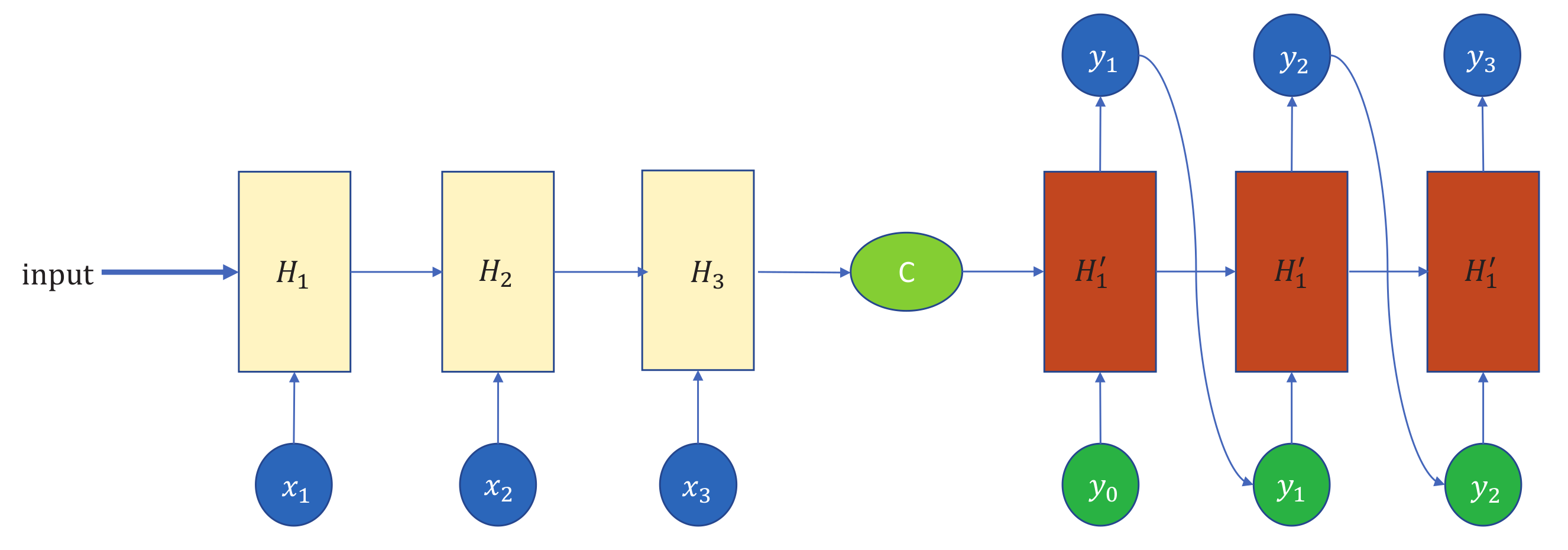
3.3. Attention with Encoder and Decoder

Unlike previous RNN models, which were plagued by the problem of short-term memory, the main feature of the LSTM is that it regulates the selection and forgetting of important and unimportant information through a sigmoid neural network layer and a “gate” structure that multiplies bit by bit. The LSTM model can handle long-term dependencies as well as gradient disappearance and explosion problems caused by long sequence training very well [48]. However, as the input data length increases, the amount of forgotten information selected by the model will inevitably gradually increase. Water quality data often cover a long time period (from one year to several years), contain high-dimensional features, and carry a lot of noise. Therefore, using LSTM models as encoders and decoders to process water quality information containing high-dimensional feature data will encounter the following problems:
(1)
The encoder LSTM only outputs the state at the last time step, which is used as the initial state for the decoder LSTM. This indicates that the model cannot fully use information from all time steps for prediction. For example, input from the last time step of a sequence cannot capture features from earlier in the sequence.
(2)
Although LSTM can handle long sequence data, when dealing with multi-dimensional covariate data, it will compress it into a context vector of fixed length. This causes the decoder to lose interactive information in multi-dimensional data, so that the decoder cannot obtain output information corresponding to different dimensional data.
The multidimensional information of covariates plays a crucial role in determining the accuracy of water quality prediction. To address this, we have incorporated an attention mechanism at the encoder layer. This computes corresponding attention weights for each output state of the decoder at each time step and multiplies them with the output vector of the decoder to obtain both label information and input covariate information. The encoder can then identify the most relevant information based on its importance and better capture high-dimensional features of the covariate information.
As shown in Figure 3, we take the vector of each time step k i (containing the covariate x i and the corresponding feature data z i ) specified by the step length k = { k 1 , k 2 , k m } , and obtain a tensor of fixed size as input to the LSTM decoder by embedding. We then obtain the hidden state h i of the encoder at time step i, as well as the current output vector Q i . We store all hidden states within a time step, and compute attention scores based on these states and the decoder state h t to determine how much weight to give to different parts of the encoder. The procedure for handling a single time step in an LSTM encoder is as follows:
O i , h i = encoder z i , x i , h i 1
h i 1 provides historical sequence information for the current time step as the previous hidden layer state, and ( z i , x i ) is the input data at the current time step. They produce the current hidden layer state h i and the output result O i . The attention layer can find correlation weights between the decoder input state and historical states to obtain a new hidden layer state that serves as input to the next decoder, while also producing prediction results on the current decoder. We illustrate how attention mechanisms work in models by processing four pieces of data starting from time step i within one time step.
As shown in Figure 4, the data at each time step within the current time step includes covariate data x i with a shape of [batchSize, hiddenSize] and corresponding feature data z i . The LSTM decoder produces an output state for each time step, which is then compared to the decoder’s current output state h i + 4 using similarity scoring. This computational method is commonly referred to as dot product attention, where the query vector h t and the target vector group h i are multiplied separately.
score h i = h t · h i
Or use the cosine similarity formula for calculation.
score h i = h t · h i h t · h i
This article uses the dot product attention calculation method to calculate the attention scores of each hidden layer. Here, we perform matrix multiplication and dot product calculation on the input data. Then, we normalise the obtained attention scores using softmax to obtain the contribution of each vector relative to the encoder’s hidden layer. Finally, we take a weighted sum of each decoder’s hidden layer contributions to obtain the current time step context vector c i for the encoder’s hidden layer. We then concatenate c i with the current decoder covariate f e a t x as input for time step t + 1 , and after linear transformation, obtain the prediction result y i + 4 for time step t. With this approach, our model dynamically adjusts its encoding inputs based on the decoder state in order to more fully exploit the information from the input sequences and avoid the loss of information caused by fixed-length sequence inputs, while exploiting high-dimensional covariate features.

3.4. KF-LSTM Based Water Quality Prediction Model

In this section we present the details of the model training and testing process. The overall processing flow of the model is divided into three steps: (1) After repairing and smoothing the raw data, the data will be partitioned and normalised according to the model parameters for convenient data processing and faster convergence. Each training round obtains fixed-length historical covariates x, historical label values z, predicted covariates x and predicted label values z from the partitioned training data. (2) All parts of the data are converted into vectors of size equal to the model parameter hiddenSize, and all hidden states obtained by the decoder at each time step are stored. The attention layer processes these states to compute weight values for each hidden layer relative to the decoder output state, thereby improving the model’s attention to key information and obtaining the output for the next time step. After each round of training, the model requires continuous parameter updates and optimisation to reduce the loss between predicted and actual values. (3) Use test sets to verify the performance of the models through multiple evaluation metrics; plot fitting graphs showing predictions versus actuals at specified time steps as further evidence of effectiveness.
Finally, we provide pseudocode describing the detailed processing flow within our model as shown in Algorithm 2, along with important parameter choices such as batch size and learning rate, as well as assumptions made regarding loss functions.
Algorithm 2: Algorithm for the prediction of water quality based on KF-LSTM
Input: 
Inputting the raw data into the Kalman filter yields smoothed Data(N*M).And preparing various hyperparameters of the model.
Output: 
y
 1:
Step 1 : Encoder
 2:
enc_state = [] hidden = []
 3:
for   i = 1 , 2 , , e n c o d e _ s t e p   do
 4:
 input_z, input_x = embeding(history_z,history_x)
 5:
 cell_input = Concatenate(input_z,input_x)
 6:
 output,hidden = LSTM(cell_input,hidden)
 7:
 Concatenate every output state of the encoder
 8:
end for
 9:
Step 2 : Decoder
 10:
last_state ← Retrieve the final output state of the decoder
 11:
future_x ← Covariates of predictive features
 12:
for   i = 1 , 2 , , e n c o d e _ s t e p   do
 13:
 use encoder_states and state and future_x to compute atteninput
 14:
 Update the hidden state of the decoder and use it as input for the next decoding step.
 15:
 output,hidden = LSTM(cell_input,update_hidden)
 16:
 Save all states of the decoder.
 17:
end for
 18:
Step 3 : Update model
 19:
The predicted results will be processed through the thread layer for output y.
 20:
Update model parameters by comparing calculation errors with actual data.
 21:
Step 4 : Prediction
 22:
Use the test set for testing and display the test results.
We explain the processing flow of the input-output interpretation model with data. After the raw data is processed by Kalman filtering, missing values are imputed and the data is normalised as input to the encoder. In an encoding step, the historical covariates x and the label variable z are extracted from the input and each undergoes an embedding transformation into a size tensor ( b a t c h _ s i z e , h i d d e n _ s i z e ), which is concatenated as cell input to the LSTM encoder. The hidden inputs are continuously updated within each encoding step, while all outputs are recorded. We then add an attention layer after the decoder to dynamically compute attention values for context vectors in each output from the encoder, and combine them with the current decoder output vector as the prediction result y for the next time step. After each training round, the model parameters are updated by backpropagation to improve its accuracy and generalisation ability. Finally, test data is used to verify the accuracy of the model.

4. Experiment

4.1. Experimental Settings

All experiments used in this paper were performed on Windows 10 Professional, version 21H2, on a computer with the following main parameters (CPU: AMD Ryzen 5 3600 6-core processor 3.60 GHz; GPU: NVIDIA GeForce GTX 1080 Ti GPU). The code was compiled using PyCharm version 2021.2.3 compiler, and the full syntax followed Python version 3.7. Our codes, parameters, and dataset are all publicly available on the Internet for scholars to refer to or verify our experimental results (https://github.com/Enki-Zhang/KFLSTM) (accessed on 3 July 2023). The results of the optimisation of the main hyperparameters for all the models used in this study are shown in Table 1.

4.2. Data Analysis and Preprocessing

The Liandjiang River, the third largest river in eastern Guangdong, has a total length of 71.1 kilometres and a drainage area of 1353 square kilometres. It covers three county-level administrative regions, including Chaoyang District and Chaonan District in Shantou City and Puning City in Jieyang. There are more than 20 major tributaries, such as Liusha Xinhe, Liusha Zhonghe, Baikeng Lake Water, Baimaxi Creek, Shuiwei Creek, Tangkeng Creek, Chendian Chong Stream Outlet, Sima Cutoff Channel, Qiufeng Waterway, Xiashan Daxi, Lugang Chong Stream, Miancheng Canal, Beigang River and Gurao Chong Stream. It has an important impact on people’s production and life. The development of the Liandjiang River Basin has been severely polluted over the past few decades due to the continuous discharge of large amounts of industrial pollution and domestic wastewater into the Liandjiang River Basin and its tributaries. Since 1998, the overall water quality of the Liandjiang River has been consistently classified as inferior class V, with more than 96% of the monitoring reaches being inferior class V. Therefore, there is an urgent need to manage the water quality of the Liandjiang River.
There are 22 monitoring sites in the Lianjiang River Basin. We used the detection data from the Haimen Bay monitoring station in the Lianjiang River system, which includes various data reflecting water quality pollution such as dissolved oxygen, pH, conductivity, turbidity, total nitrogen, total phosphorus, hexavalent chromium, sulphide, cyanide, volatile phenols and potassium permanganate index (Figure 5). The geographical location of Haimen Bay is shown in the figure. However, due to the different characteristics of different indicators, the data characteristics and monitoring frequency at each site for different indicators are not the same. Selecting water quality indicators with the same monitoring frequency as the model input is a basic requirement for modelling. Therefore, we selected five data indicators (pH, temperature, dissolved oxygen, conductivity, turbidity) with a monitoring frequency of one hour at all sites containing all available data from 1 January 2019 to 30 June 2020, totaling 13,128 pieces of data, and performed Pearson correlation coefficient analysis on these five types of data as shown in Figure 6. Blue indicates positive correlation; red indicates negative correlation; white indicates no correlation. The figure shows that there is a good correlation between these five types of data; therefore pH, temperature, dissolved oxygen, conductivity and turbidity can be used as model inputs.
The data statistics presented in Table 2 show the common options for statistical data such as total number of data, mean value, extreme values of the data, number of missing values in each item and units of measurement. Due to various uncontrollable factors such as equipment failure, it is often difficult to obtain accurate and continuous readings from monitoring stations. After statistical analysis, we found that there were 1894 missing values during the monitoring process over a period of eighteen months. This has a significant impact on subsequent predictions and is an issue that needs attention.
We will use a Kalman filter to perform optimal estimation on the data to be processed to fill in missing values. Due to the long time span and the large amount of data, we have only selected different water quality characteristics with missing values between 8345–8945 and their results after filtering by the Kalman filter as an example to demonstrate its effectiveness, as shown in Figure 7. Taking the dissolved oxygen index data as an example (other index data have similar dissolved oxygen processing effects), the main positions where there are missing values in the data are 8423–8440, 8462–8466, 8552–8593, 8645–8664 and 8682–8728. The figure shows that while the Kalman filter fills in the missing values (indicated by the light blue curve), it also performs smoothing noise reduction on the original data (indicated by the red curve).

4.3. Model Evaluation Metrics

This section introduces the selection of evaluation criteria for the model. We use several commonly used evaluation indicators for regression models to evaluate the model from different perspectives. Mean Absolute Error (MAE) is used to measure the average absolute error between predicted values and true values, where y i is the true value of sample i, y ^ i is the predicted value of sample i, and n is the number of samples. The MAE can better reflect the prediction error situation, and a smaller MAE indicates a better predictive ability of the model [49].
M A E = 1 n i = 1 n y i y ^ i
Mean Squared Error (MSE) [50] is a measure of the quality of a model, calculated by dividing the sum of squares of the errors by the total number of predicted data. The smaller the value, the better the predictive ability of the model. In this formula, y i is the true value for data point i, y ^ i is its predicted value, and n is the sample size.
M S E = 1 n i = 1 n y i y ^ i 2
Root Mean Square Error (RMSE) [51], usually obtained by taking the square root of the MSE to convert the error into a form that is in the same units as the original data. It is easier to understand than the MSE. This formula is used to indicate how much error the model will produce in the prediction. For larger errors, the weight is higher, which means that as the RMSE value increases, it indicates poorer predictive performance.
R M S E = 1 n i = 1 n y i y ^ i 2
R 2 , also known as the coefficient of determination, is the default indicator used by sklearn for regression analysis. The value of R 2 reflects the quality of fit of the model. In the formula, y ¯ represents the average of the actual values.
R 2 = 1 i = 1 n y i y ^ i 2 i = 1 n y i y ¯ 2

Hyperparameter Optimization and Cross-Validation

The values of the model’s hyperparameters determine the model’s final prediction performance and generalisation ability. Therefore, optimising the hyperparameters for each model is an essential part of machine learning. Grid search is a simple and effective method for selecting hyperparameters. Due to our small dataset and to avoid overfitting, we used k-fold cross-validation in the hyperparameter selection process. We divided 80% of the data as a training set and 20% as a test set, then performed cross-validation on the training set by dividing it into k non-overlapping subsets, using k − 1 subsets to fit the model, and validating it with the remaining subset. This was repeated k times to obtain an average result from k experimental results [52]. In this study, given the characteristics of a small dataset, we used 5-fold cross-validation (k = 5) combined with grid search to complete the hyperparameter optimisation of our models. In each iteration, the training set was randomly divided into five parts and trained on four parts, while one part was used as test data, so that each subset served as a test set once. The final performance of our models was determined by averaging the results of all five test sets.
Table 1 presents the hyperparameter optimization results for all models in this study. All models in the table underwent hyperparameter optimization using the training set, with M S E as the optimization metric. For the MLP model, the hyperparameter optimization included learning rate (0.001, 0.01, 0.1), number of hidden layers (32, 64, 128), and maximum iteration number (200, 300, 400, 500, 600, 700, 800). The hyperparameters for the Classification and Regression Tree (CART) model included maximum tree depth (10, 15, 20, 25, 30), minimum sample required to split internal nodes (2, 3, 4, 5, 10), and minimum sample required at leaf nodes (2, 3, 4, 5, 6). The optimization hyperparameters for Random Forest were maximum tree depth (10, 20, 30, 40) and number of decision trees (20, 40, 50, 60, 70, 80, 90, 100, 120, 150). XGBoost’s optimization hyperparameters were learning rate (0.001, 0.01, 0.1), maximum tree depth (3, 5, 7, 9), and number of trees used by the model (100, 200, 300, 400, 500). The hyperparameters for KF-GRU and KF-LSTM models included sequence structure in the Kalman filter, target quantity in the model(1), number of feature columns(4), hidden layer size (1, 2, 3, 4), encoder-decoder layer numbers (1, 2, 3, 4), dropout rate regularization size (0.2, 0.3, 0.4, 0.5, 0.6, 0.7, 0.8), encoder and decoder size (1, 2, 3, 4), batch size(2, 4, 8, 16, 32, 64, 128), and learning rate (0.1, 0.01, 0.001). In the next section, we will discuss the performance of each model on the training and test sets.

4.4. Experiment Results

We compared the MLP, Lassification and Regression Trees (CART), RF, XGBoost, and KF-GRU models with our encoder-decoder replaced by the GRU model and the KF-LSTM as comparison models to jointly validate the experimental data, using the same data and data partitioning with hyperparameter optimisation and cross-validation. The input data of the MLP, CART, RF and XGBoost models were only zero-filled and normalised.
Table 3 shows the experimental results of all models in the training and test set, respectively. From Table 3 we can see that KF-LSTM outperforms the other models in both the training and the test set, with the scores of each metric in the test set, which is a variant of the LSTM, and that the lower scores of the model are justified by the particular nature of the data used in the model, which makes it difficult for traditional machine learning models to learn the characteristics of long-term data. As shown in the table, the R 2 values of the MLP, CART, RF, XGBoost, KF-GRU, KF-LSTM models on the test set are 0.30, 0.57, 0.67, 0.77, 0.87, 0.94 respectively.
The performance of the KF-LSTM and KF-GRU models in predicting the last 72 time steps is shown in Figure 8. It can be seen from Figure 8 that the overall fitting effect of the KF-GRU model is slightly weaker than that of the KF-LSTM model, and the prediction deviation is most evident in the range of 0 to 25 time steps. The KF-LSTM model can better fit the trend of the test data.
The Figure 9 illustrates the comparison between the predicted and actual values of dissolved oxygen content by different models (a–f) on the training and test sets. The presence of noise in water quality data and a high number of missing values can significantly affect the performance of the models. From the figure, it can be observed that the predicted values of KF-LSTM are more concentrated around the Y = X line, indicating the highest predictive ability. KF-LSTM exhibits the lowest values of M A E , M S E , R M S E , and the highest value of R 2 (10). On the other hand, the MLP model performs the worst among all the models.
At the same time, we found that LSTM is more suitable for processing larger amounts of data than GRU variants using LSTM, because traditional RNN models are difficult to learn long-term features due to their particular case-specificity, resulting in less-than-ideal scores across various metrics.

4.5. Ablation Experiment

To provide a more obvious quantitative comparison and to verify the effectiveness of the Kalman filter on the model, we conducted experiments on different models, including the LSTM-seq2seq model without filters, the GRU-seq2seq model with the encoder changed to GRU, and the KF-LSTM model. We obtained the prediction effects of different models on DO as shown in Figure 10. The horizontal x-axis represents the observed values, while the vertical y-axis represents the predicted values. If a model’s error follows a Gaussian distribution, its data will be distributed along the Y = X line or equally on either side of it. The closer the data are to the Y = X line, the smaller the prediction error. From Figure 10 it can be seen that LSTM-seq2seq and GRU-seq2seq are far from the Y = X line, and LSTM-seq2seq tends to be distributed more to one side of the Y = X line, indicating larger bias errors that may result from overfitting or underfitting. Therefore, we conclude that KF-LSTM and KF-GRU have better performance in predicting dissolved oxygen index data with M A E of 0.31 and 0.47 respectively; Kalman filter module can improve the predictive performance of dissolved oxygen data.

4.6. Optimizer Selection and Parameter Optimization

In this section we discuss the impact of different optimisers on the loss during model training. The choice of optimiser is crucial for the model as it can update different parameters of the loss function during backpropagation to reach a local optimum. We compared the performance of different gradient-based optimisers, including Adam, AdamW, Adagrad, SGD and Adadelta, in terms of loss over 20 epochs, as shown in Figure 11. The losses for all these optimisers decreased continuously and gradually stabilised with increasing epochs. The final losses for each optimiser were AdamW = 0.0157, Adam = 0.0268, Adagrad = 0.1727, SGD = 0.232 and Adadelta = 0.2583 respectively. Therefore, we chose AdamW as the optimiser of our model because its loss was slightly lower than that of Adam, possibly due to the addition of a weight decay regularisation term during backpropagation, which improved the computational efficiency [53].
Having discussed the choice of optimiser, we need to move on to two important hyperparameters in the model: batch size and learning rate. The batch size setting represents the number of samples trained by the model in an epoch, while the learning rate reflects the degree of adjustment of the model parameters as model errors are updated each time. In deep learning models, the stochastic gradient descent algorithm is generally used for optimisation. The formula for updating model weights can be expressed as
w t + 1 = w t η m i m J ( w t )
where η is the size of the learning rate, m is the size of the batch size, J ( w t ) is the gradient of the loss function J to the weight w t , subtracting part of the average gradient from the current weight w t to get a new weight w t + 1 . From the formula, it can be seen that the learning rate and batch size are closely related and mutually influence the final effect of the model.
We continuously varied the model parameters batch size (2, 4, 8, 16, 32, 64, 128) and learning rate (0.1, 0.01, 0.001) over multiple experiments to obtain the results shown in Figure 12. We normalised the M A E results of each experiment to a range between 0 and 1 and mapped them to corresponding colours. The minimum M A E value is represented by the darkest green colour, while the maximum M A E value is represented by the brightest yellow colour. This creates a gradient effect from yellow to green. From our experiments, we found that setting the learning rate too high can cause the model to learn suboptimal weights too quickly or result in an unstable training process. In addition, different batch sizes have different effects on model performance, as evidenced by significant changes in adjacent colour areas and large fluctuations in image output. Based on our results graph, we determined that for optimal M A E data values of batch size = 8 and learning rate = 0.001 should be used, resulting in a dark green coloured model with an M A E of 0.38, giving us optimal performance.

5. Conclusions and Future Work

In this study, the water quality test data from 1 January 2019 to 30 June 2020, which contains a large number of missing values, are analysed and processed according to the characteristics of the water quality monitoring station in the Lienjiang River waters of Haimen Bay. However, the existing machine learning models are limited in their ability to process the data, and the variability of the prediction results is not sufficient to meet the requirements of dissolved oxygen prediction accuracy. By selecting key water quality indicators (temperature, PH, conductivity, turbidity) to construct data samples and completing the pre-processing of data from the Haimen Bay monitoring station, the model is adjusted and learned through the parameter adjustment process to complete the prediction of dissolved oxygen water quality indicators. This study also presents the prediction results of several existing machine models and compares them with the proposed model using a unified evaluation criterion:
1.
Compared with existing machine models, the method proposed in this study has the most accurate prediction of dissolved oxygen content in the water quality of Haimen Bay, with R 2 results of 0.95 and 0.94 on the training and test sets, respectively, both higher than other models, while M A E results of 0.31 and 0.30 on the training and test sets, respectively, are lower than other models.
2.
On the one hand, the treatment of missing values in the original data is different from the previous treatment, but the Kalman filter is used to best estimate the data to fill in the missing values in the data, which reduces the harshness of the model for water quality test data and improves the wide applicability of the model.
3.
On the other hand, the model uses the traditional encoder and decoder architecture, using the attention mechanism combined with LSTM neural networks to effectively alleviate the forgetting problem arising from long sequence inputs and to capture the feature interaction information of multi-dimensional covariates, thus reducing the limitations of the traditional decoder-encoder architecture.
The KF-LSTM model has a wide range of applications for predicting real-world water quality data, providing a new solution for future water quality management and environmental protection in smart cities, as well as helping to solve natural language processing (NLP) challenges.
This study mainly focuses on the prediction of a single variable of water quality in the Lianjiang River, which is a limitation of the model now, but the data indicators of other dimensions in water quality are equally important and together reflect the comprehensive situation of the water body, so future work will try different attention mechanisms to achieve the goal from multivariate prediction of a single variable to multivariate prediction of multiple variables to improve the accuracy of the model for water quality prediction, While in the current prediction process, we only selected the water quality of one monitoring station in Lianjiang River for prediction, in the future research progress, we will try to predict the water quality with different data from several monitoring stations in Lianjiang River (Qingyangshan Bridge, Jingzaiwan Gate and Heping Bridge).

Author Contributions

Conceptualization, H.C.; data curation, C.Z., L.X., S.H. and Y.Z.; formal analysis, C.Z. and J.X.; investigation, L.X., S.H. and Y.Z.; methodology, H.C., C.Z., J.X. and F.W.; validation, F.W.; writing—original draft, H.C., C.Z. and J.X. All authors have read and agreed to the published version of the manuscript.

Funding

This study was funded by Guangdong province special fund for science and technology (“major special projects + task list”) project (No. STKJ2021201, STKJ2021011, STKJ202209017, STKJ2021021), the 2020 Li Ka Shing Foundation Cross-Disciplinary Research Grant (No. 2020LKSFG08D), Special Projects in Key Fields of Guangdong Universities (No. 2022ZDZX1008), and part by the Guangdong Basic and Applied Basic Research Foundation (No. 2023A1515010707).

Data Availability Statement

Not applicable.

Conflicts of Interest

The authors declare no conflict of interest.

References

  1. Morin-Crini, N.; Lichtfouse, E.; Liu, G.; Balaram, V.; Ribeiro, A.R.L.; Lu, Z.; Stock, F.; Carmona, E.; Teixeira, M.R.; Picos-Corrales, L.A.; et al. Worldwide Cases of Water Pollution by Emerging Contaminants: A Review. Environ. Chem. Lett. 2022, 20, 2311–2338. [Google Scholar] [CrossRef]
  2. Tang, W.; Pei, Y.; Zheng, H.; Zhao, Y.; Shu, L.; Zhang, H. Twenty Years of China’s Water Pollution Control: Experiences and Challenges. Chemosphere 2022, 295, 133875. [Google Scholar] [CrossRef] [PubMed]
  3. Xue, J.; Wang, Q.; Zhang, M. A Review of Non-Point Source Water Pollution Modeling for the Urban–Rural Transitional Areas of China: Research Status and Prospect. Sci. Total Environ. 2022, 826, 154146. [Google Scholar] [CrossRef] [PubMed]
  4. Alasri, T.M.; Ali, S.L.; Salama, R.S.; Alshorifi, F.T. Band-Structure Engineering of TiO2 Photocatalyst by AuSe Quantum Dots for Efficient Degradation of Malachite Green and Phenol. J. Inorg. Organomet. Polym. Mater. 2023. [Google Scholar] [CrossRef]
  5. Mostafa, M.M.M.; Alshehri, A.A.; Salama, R.S. High performance of supercapacitor based on alumina nanoparticles derived from Coca-Cola cans. J. Energy Storage 2023, 64, 107168. [Google Scholar] [CrossRef]
  6. Kutty, A.A.; Wakjira, T.G.; Kucukvar, M.; Abdella, G.M.; Onat, N.C. Urban Resilience and Livability Performance of European Smart Cities: A Novel Machine Learning Approach. J. Clean. Prod. 2022, 378, 134203. [Google Scholar] [CrossRef]
  7. Chen, Y.; Song, L.; Liu, Y.; Yang, L.; Li, D. A Review of the Artificial Neural Network Models for Water Quality Prediction. Appl. Sci. 2020, 10, 5776. [Google Scholar] [CrossRef]
  8. Tian, X.; Wang, Z.; Taalab, E.; Zhang, B.; Li, X.; Wang, J.; Ong, M.C.; Zhu, Z. Water Quality Predictions Based on Grey Relation Analysis Enhanced LSTM Algorithms. Water 2022, 14, 3851. [Google Scholar] [CrossRef]
  9. Ye, Q.; Yang, X.; Chen, C.; Wang, J. River Water Quality Parameters Prediction Method Based on LSTM-RNN Model. In Proceedings of the 2019 Chinese Control And Decision Conference (CCDC), Nanchang, China, 3–5 June 2019; pp. 3024–3028. [Google Scholar] [CrossRef]
  10. Hussein, A.M.; Abd Elaziz, M.; Abdel Wahed, M.S.; Sillanpää, M. A New Approach to Predict the Missing Values of Algae during Water Quality Monitoring Programs Based on a Hybrid Moth Search Algorithm and the Random Vector Functional Link Network. J. Hydrol. 2019, 575, 852–863. [Google Scholar] [CrossRef]
  11. Najah Ahmed, A.; Binti Othman, F.; Abdulmohsin Afan, H.; Khaleel Ibrahim, R.; Ming Fai, C.; Shabbir Hossain, M.; Ehteram, M.; Elshafie, A. Machine Learning Methods for Better Water Quality Prediction. J. Hydrol. 2019, 578, 124084. [Google Scholar] [CrossRef]
  12. Shahriari, S.; Sisson, S.; Rashidi, T. Copula ARMA-GARCH Modelling of Spatially and Temporally Correlated Time Series Data for Transportation Planning Use. Transp. Res. Part C Emerg. Technol. 2023, 146, 103969. [Google Scholar] [CrossRef]
  13. Zhao, Z.; Zhai, M.; Li, G.; Gao, X.; Song, W.; Wang, X.; Ren, H.; Cui, Y.; Qiao, Y.; Ren, J.; et al. Study on the Prediction Effect of a Combined Model of SARIMA and LSTM Based on SSA for Influenza in Shanxi Province, China. BMC Infect. Dis. 2023, 23, 71. [Google Scholar] [CrossRef]
  14. Dai, H.; Huang, G.; Wang, J.; Zeng, H. VAR-tree Model Based Spatio-Temporal Characterization and Prediction of O3 Concentration in China. Ecotoxicol. Environ. Saf. 2023, 257, 114960. [Google Scholar] [CrossRef] [PubMed]
  15. Kurani, A.; Doshi, P.; Vakharia, A.; Shah, M. A Comprehensive Comparative Study of Artificial Neural Network (ANN) and Support Vector Machines (SVM) on Stock Forecasting. Ann. Data Sci. 2023, 10, 183–208. [Google Scholar] [CrossRef]
  16. Alim, M.; Ye, G.H.; Guan, P.; Huang, D.S.; Zhou, B.S.; Wu, W. Comparison of ARIMA Model and XGBoost Model for Prediction of Human Brucellosis in Mainland China: A Time-Series Study. BMJ Open 2020, 10, e039676. [Google Scholar] [CrossRef]
  17. Gai, R.; Zhang, H. Prediction Model of Agricultural Water Quality Based on Optimized Logistic Regression Algorithm. EURASIP J. Adv. Signal Process. 2023, 2023, 21. [Google Scholar] [CrossRef]
  18. Liaw, A.; Wiener, M. Classification and Regression by randomForest. R News 2002, 2, 18–22. [Google Scholar]
  19. Ho, J.Y.; Afan, H.A.; El-Shafie, A.H.; Koting, S.B.; Mohd, N.S.; Jaafar, W.Z.B.; Lai Sai, H.; Malek, M.A.; Ahmed, A.N.; Mohtar, W.H.M.W.; et al. Towards a Time and Cost Effective Approach to Water Quality Index Class Prediction. J. Hydrol. 2019, 575, 148–165. [Google Scholar] [CrossRef]
  20. Lu, H.; Ma, X. Hybrid Decision Tree-Based Machine Learning Models for Short-Term Water Quality Prediction. Chemosphere 2020, 249, 126169. [Google Scholar] [CrossRef] [PubMed]
  21. Wakjira, T.G.; Rahmzadeh, A.; Alam, M.S.; Tremblay, R. Explainable Machine Learning Based Efficient Prediction Tool for Lateral Cyclic Response of Post-Tensioned Base Rocking Steel Bridge Piers. Structures 2022, 44, 947–964. [Google Scholar] [CrossRef]
  22. Giri, S.; Kang, Y.; MacDonald, K.; Tippett, M.; Qiu, Z.; Lathrop, R.G.; Obropta, C.C. Revealing the Sources of Arsenic in Private Well Water Using Random Forest Classification and Regression. Sci. Total Environ. 2023, 857, 159360. [Google Scholar] [CrossRef] [PubMed]
  23. Xu, J.; Xu, Z.; Kuang, J.; Lin, C.; Xiao, L.; Huang, X.; Zhang, Y. An Alternative to Laboratory Testing: Random Forest-Based Water Quality Prediction Framework for Inland and Nearshore Water Bodies. Water 2021, 13, 3262. [Google Scholar] [CrossRef]
  24. Ghose, D.K.; Panda, S.S.; Swain, P.C. Prediction of Water Table Depth in Western Region, Orissa Using BPNN and RBFN Neural Networks. J. Hydrol. 2010, 394, 296–304. [Google Scholar] [CrossRef]
  25. Wang, H.Y.; Chen, B.; Pan, D.; Lv, Z.A.; Huang, S.Q.; Khayatnezhad, M.; Jimenez, G. Optimal Wind Energy Generation Considering Climatic Variables by Deep Belief Network (DBN) Model Based on Modified Coot Optimization Algorithm (MCOA). Sustain. Energy Technol. Assessments 2022, 53, 102744. [Google Scholar] [CrossRef]
  26. Sharif, S.M.; Kusin, F.M.; Asha’ari, Z.H.; Aris, A.Z. Characterization of Water Quality Conditions in the Klang River Basin, Malaysia Using Self Organizing Map and K-means Algorithm. Procedia Environ. Sci. 2015, 30, 73–78. [Google Scholar] [CrossRef] [Green Version]
  27. Csábrági, A.; Molnár, S.; Tanos, P.; Kovács, J. Application of Artificial Neural Networks to the Forecasting of Dissolved Oxygen Content in the Hungarian Section of the River Danube. Ecol. Eng. 2017, 100, 63–72. [Google Scholar] [CrossRef]
  28. Lee, S.; Kim, J. Predicting Inflow Rate of the Soyang River Dam Using Deep Learning Techniques. Water 2021, 13, 2447. [Google Scholar] [CrossRef]
  29. Hochreiter, S.; Schmidhuber, J. Long Short-Term Memory. Neural Comput. 1997, 9, 1735–1780. [Google Scholar] [CrossRef]
  30. Liu, C.; Liu, D.; Mu, L. Improved Transformer Model for Enhanced Monthly Streamflow Predictions of the Yangtze River. IEEE Access 2022, 10, 58240–58253. [Google Scholar] [CrossRef]
  31. Tao, Q.; Liu, F.; Li, Y.; Sidorov, D. Air Pollution Forecasting Using a Deep Learning Model Based on 1D Convnets and Bidirectional GRU. IEEE Access 2019, 7, 76690–76698. [Google Scholar] [CrossRef]
  32. Ma, X.; Tao, Z.; Wang, Y.; Yu, H.; Wang, Y. Long Short-Term Memory Neural Network for Traffic Speed Prediction Using Remote Microwave Sensor Data. Transp. Res. Part C Emerg. Technol. 2015, 54, 187–197. [Google Scholar] [CrossRef]
  33. Liu, P.; Wang, J.; Sangaiah, A.; Xie, Y.; Yin, X. Analysis and Prediction of Water Quality Using LSTM Deep Neural Networks in IoT Environment. Sustainability 2019, 11, 2058. [Google Scholar] [CrossRef] [Green Version]
  34. Yang, J.; Zhao, K.; Yu, X.; Yan, Y.; He, Z.; Lai, Y.; Zhou, Y. Crack Classification of Fiber-Reinforced Backfill Based on Gaussian Mixed Moving Average Filtering Method. Cem. Concr. Compos. 2022, 134, 104740. [Google Scholar] [CrossRef]
  35. Ahmed, H.; Ullah, A. Exponential Moving Average Extended Kalman Filter for Robust Battery State-of-Charge Estimation. In Proceedings of the 2022 International Conference on Innovations in Science, Engineering and Technology (ICISET), Chittagong, Bangladesh, 26–27 February 2022; pp. 555–560. [Google Scholar] [CrossRef]
  36. Hamzah, F.B.; Mohd Hamzah, F.; Mohd Razali, S.F.; Samad, H. A Comparison of Multiple Imputation Methods for Recovering Missing Data in Hydrological Studies. Civ. Eng. J. 2021, 7, 1608–1619. [Google Scholar] [CrossRef]
  37. Banerjee, K.; Bali, V.; Nawaz, N.; Bali, S.; Mathur, S.; Mishra, R.K.; Rani, S. A Machine-Learning Approach for Prediction of Water Contamination Using Latitude, Longitude, and Elevation. Water 2022, 14, 728. [Google Scholar] [CrossRef]
  38. Xu, J.; Wang, K.; Lin, C.; Xiao, L.; Huang, X.; Zhang, Y. FM-GRU: A Time Series Prediction Method for Water Quality Based on Seq2seq Framework. Water 2021, 13, 1031. [Google Scholar] [CrossRef]
  39. Liu, Y.; Tian, W.; Xie, J.; Huang, W.; Xin, K. LSTM-Based Model-Predictive Control with Rationality Verification for Bioreactors in Wastewater Treatment. Water 2023, 15, 1779. [Google Scholar] [CrossRef]
  40. Kalman, R.E. A New Approach to Linear Filtering and Prediction Problems. J. Basic Eng. 1960, 82, 35–45. [Google Scholar] [CrossRef] [Green Version]
  41. Bakibillah, A.; Tan, Y.H.; Loo, J.Y.; Tan, C.P.; Kamal, M.; Pu, Z. Robust Estimation of Traffic Density with Missing Data Using an Adaptive-R Extended Kalman Filter. Appl. Math. Comput. 2022, 421, 126915. [Google Scholar] [CrossRef]
  42. Cai, L.; Zhang, Z.; Yang, J.; Yu, Y.; Zhou, T.; Qin, J. A Noise-Immune Kalman Filter for Short-Term Traffic Flow Forecasting. Phys. A Stat. Mech. Its Appl. 2019, 536, 122601. [Google Scholar] [CrossRef]
  43. Momin, K.A.; Barua, S.; Jamil, M.S.; Hamim, O.F. Short Duration Traffic Flow Prediction Using Kalman Filtering. In Proceedings of the 6th International Conference on Civil Engineering for Sustainable Development (ICCESD 2022), Khulna, Bangladesh, 10–12 February 2022; p. 040011. [Google Scholar] [CrossRef]
  44. Sutskever, I.; Vinyals, O.; Le, Q.V. Sequence to Sequence Learning with Neural Networks. arXiv 2014, arXiv:1409.3215. [Google Scholar]
  45. Dey, R.; Salem, F.M. Gate-variants of Gated Recurrent Unit (GRU) neural networks. In Proceedings of the 2017 IEEE 60th International Midwest Symposium on Circuits and Systems (MWSCAS), Boston, MA, USA, 6–9 August 2017; pp. 1597–1600. [Google Scholar] [CrossRef] [Green Version]
  46. Vaswani, A.; Shazeer, N.; Parmar, N.; Uszkoreit, J.; Jones, L.; Gomez, A.N.; Kaiser, L.; Polosukhin, I. Attention Is All You Need. arXiv 2017, arXiv:cs/1706.03762. [Google Scholar]
  47. Pan, M.; Zhou, H.; Cao, J.; Liu, Y.; Hao, J.; Li, S.; Chen, C.H. Water Level Prediction Model Based on GRU and CNN. IEEE Access 2020, 8, 60090–60100. [Google Scholar] [CrossRef]
  48. Yu, Y.; Si, X.; Hu, C.; Zhang, J. A Review of Recurrent Neural Networks: LSTM Cells and Network Architectures. Neural Comput. 2019, 31, 1235–1270. [Google Scholar] [CrossRef] [PubMed]
  49. Willmott, C.; Matsuura, K. Advantages of the Mean Absolute Error (MAE) over the Root Mean Square Error (RMSE) in Assessing Average Model Performance. Clim. Res. 2005, 30, 79–82. [Google Scholar] [CrossRef]
  50. Abobakr Yahya, A.S.; Ahmed, A.N.; Binti Othman, F.; Ibrahim, R.K.; Afan, H.A.; El-Shafie, A.; Fai, C.M.; Hossain, M.S.; Ehteram, M.; Elshafie, A. Water Quality Prediction Model Based Support Vector Machine Model for Ungauged River Catchment under Dual Scenarios. Water 2019, 11, 1231. [Google Scholar] [CrossRef] [Green Version]
  51. Aklilu, E.G.; Adem, A.; Kasirajan, R.; Ahmed, Y. Artificial Neural Network and Response Surface Methodology for Modeling and Optimization of Activation of Lactoperoxidase System. S. Afr. J. Chem. Eng. 2021, 37, 12–22. [Google Scholar] [CrossRef]
  52. Wakjira, T.G.; Ibrahim, M.; Ebead, U.; Alam, M.S. Explainable Machine Learning Model and Reliability Analysis for Flexural Capacity Prediction of RC Beams Strengthened in Flexure with FRCM. Eng. Struct. 2022, 255, 113903. [Google Scholar] [CrossRef]
  53. You, Y.; Li, J.; Reddi, S.; Hseu, J.; Kumar, S.; Bhojanapalli, S.; Song, X.; Demmel, J.; Keutzer, K.; Hsieh, C.J. Large Batch Optimization for Deep Learning: Training BERT in 76 Minutes. arXiv 2020, arXiv:1904.00962. [Google Scholar]
Figure 1. Encoder-Decoder structure.
Water 15 02542 g001
Figure 2. Metrics for different models.
Water 15 02542 g002
Figure 3. Attention with Encoder and Decoder.The data at each time step is input into the LSTM module of the encoder, and all hidden layer output vectors from each time step are combined. The weights of the encoder output are calculated through an attention mechanism using both the combined hidden layer output vectors and the decoder’s LSTM module output vector. This updates the decoder’s state to obtain its current prediction.
Water 15 02542 g003
Figure 4. Attention Mechanism Model Diagram.
Water 15 02542 g004
Figure 5. LianJiangRiver and Haimen Bay Monitoring Station.
Water 15 02542 g005
Figure 6. Explanation of Water Quality Data Correlation.
Water 15 02542 g006
Figure 7. The comparison of the filtering effect of the Kalman filter, where the red part is the original data and the blue part is the filtered data processed by the Kalman filter.
Water 15 02542 g007
Figure 8. Comparison of dissolved oxygen fitting within the last 72 time steps.
Water 15 02542 g008
Figure 9. Comparison of dissolved oxygen predictions from different models on training and test sets.
Water 15 02542 g009
Figure 10. The prediction results of the last 72 time steps for water quality prediction using different models.
Water 15 02542 g010
Figure 11. The loss curves with different optimizers.
Water 15 02542 g011
Figure 12. Optimization of Learning Rate and Batch Size.
Water 15 02542 g012
Table 1. The optimized values of hyperparameters for different models.
ModelHyperparameterOptimal Value
Multilayer PerceptronLearning rate0.001
Hidden layers Sizes32
Maximum number of iterations700
Classification and Regression TreeMaximum depth of tree20
Minimum number of samples required to be at a leaf node8
Minimum number of samples required to split an internal node4
Divisive strategyBest
Random ForestMaximum depth10
Maximum number of estimators90
XGBoostLearning Rate0.1
Maximum depth of tree7
Maximum number of estimators300
KF-GRUTiming structure of the Kalman filterlevel_trend
Target size1
Feature size4
Hidden layers Sizes128
The number of layers in GRU2
Dropout rate0.2
Encode steps24
Forcast steps12
Batch size6
Learning rate0.001
KF-LSTMTiming structure of the Kalman filterlevel_trend
Target size1
Feature size4
Hidden layers Sizes128
The number of layers in LSTM3
Dropout rate0.3
Encode steps24
Forcast steps12
Batch size8
Learning rate0.001
Table 2. Monitoring station water quality information statistics.
Water DataCountMeanNumber of Missing ValuesMinimum ValueMaximum ValueUnit
Temperature12,75724.6553711535°C
PH12,7527.40123763.639.86-
Electrical12,7634596.68365446,878μs/cm
Turbidity12,76455.193641500NTU
DO12,7105.23664180.0515mg/L
Table 3. Comparison of prediction performance of different models for dissolved oxygen levels.
DataMetricsModel
MLPCARTRFXGBoostKF-GRUKF-LSTM
Train set M A E 1.751.151.120.870.440.31
M S E 5.272.712.321.540.430.15
R M S E 2.291.641.521.240.650.38
R 2 0.280.630.680.830.880.95
Test set M A E 1.731.351.160.950.470.30
M S E 5.273.302.511.810.410.16
R M S E 2.291.811.581.340.620.40
R 2 0.300.570.670.770.870.94
Disclaimer/Publisher’s Note: The statements, opinions and data contained in all publications are solely those of the individual author(s) and contributor(s) and not of MDPI and/or the editor(s). MDPI and/or the editor(s) disclaim responsibility for any injury to people or property resulting from any ideas, methods, instructions or products referred to in the content.

