Article

Analysis of Seasonal Driving Factors and Inversion Model Optimization of Soil Moisture in the Qinghai Tibet Plateau Based on Machine Learning

1
College of Earth Science and Engineering, Shandong University of Science and Technology, Qingdao 266590, China
2
Shandong Province Research Institute of Coal Geology Planning and Exploration, Jinan 250104, China
*
Author to whom correspondence should be addressed.
Water 2023, 15(16), 2859; https://doi.org/10.3390/w15162859
Submission received: 9 July 2023 / Revised: 3 August 2023 / Accepted: 5 August 2023 / Published: 8 August 2023

Abstract

:
The accuracy of soil moisture retrieval based on traditional microwave remote sensing models in the Qinghai Tibet Plateau (QTP) is unstable due to its unique plateau climate. However, considering the impact of multiple multi-scale factors effectively improves the accuracy and stability of soil moisture inversion. This article uses Sentinel-1 and seasonal climate data to analyze factors and influencing mechanisms of soil moisture in the QTP. First, an artificial neural network (ANN) was used to conduct a significance analysis to screen significant influencing factors to reduce the redundancy of the experimental design and insert information. Second, the normalization effect of each factor on the soil moisture inversion was determined, and the factors with significant normalization influences were input to fit the model. Third, different fitting methods combined the semi-empirical models for soil moisture inversion. The decision tree Chi-square Automatic Interaction Detector (CHAID) analyzed the model accuracy, and the Pearson correlation coefficient between the sample and measured data was tested to further validate the accuracy of the results to obtain an optimized model that effectively inverts soil moisture. Finally, the influencing mechanisms of various factors in the optimization model were analyzed. The results show that: (1) The terrain factors, such as elevation, slope gradient, aspect, and angle, along with climate factors, such as temperature and precipitation, all have the greatest normalized impact on soil moisture in the QTP. (2) For spring (March), summer (June), and autumn (September), the greatest normalized factor of soil moisture is the terrain factor. In winter (December), precipitation was the greatest factor due to heavy snow cover and permafrost. (3) Analyzing the impact mechanism from various factors on the soil moisture showed a restricted relationship between the inversion results and the accuracy of the power fitting model, meaning it is unsuitable for general soil moisture inversion. However, among the selected models, the accuracy of the linear fit was generally higher than 79.2%, the Pearson index was greater than 0.4, and the restricted relationship between the inversion results and accuracy was weak, making it suitable for the general inversion of soil moisture in the QTP.

1. Introduction

Moisture is important in soil science research, as it significantly impacts soil nutrients, global water resources, energy cycling, and local climates [1]. Soil moisture links energy feedback between the land and atmosphere and is essential in production activities, such as the geochemical energy cycle, runoff calculations, and crop yield estimations [2,3]. Research shows that soil moisture is related to the basic attributes of soil density, texture, and structure, while being closely related to the biological soil–plant–atmosphere interactions. These interactions are usually expressed from regional climate characteristics, showing spatiotemporal heterogeneity related to the region and climate [4].
The Qinghai Tibet Plateau (QTP) has the highest elevation in the world and the largest land area in China. It has an extremely cold climate and is known as the “Roof of the World” and “Third Pole”. The QTP spans a wide range of latitudes and longitudes, with significant differences in its climate distribution [5]. Due to its high elevation and climate environment, soil moisture studies in the QTP are sensitive to geography, location, and climate [6]. The QTP also holds rich habitats, biological species, and freshwater resources, making soil science research more meaningful. However, seasonally frozen soil affects its stability, making soil moisture measurements and inversion more difficult [7]. With global warming intensifying, the permafrost in the plateau has begun to deteriorate. Monitoring soil moisture is vital to provide a reliable basis for soil scientific research within the QTP [8].
Traditional soil moisture measurement methods do not reduce the difficulty of continuous large-scale monitoring. At the same time, the development of remote sensing earth observations has provided a way to quickly obtain data with timeliness and on large scales [9]. Due to its full-time and all-weather working characteristics and the advantages of strong penetration and low atmospheric interference, microwave remote sensing has been widely used for soil moisture retrieval on large-scale bare and vegetation-covered surfaces [10,11]. Commonly used microwave remote sensing models, such as the Dubois, Oh, and Shi model, are based on radar observations with numerical simulations to calculate soil moisture [5,12,13]. For bare surfaces, the integral equation model (IEM) was proposed to broaden the scope of removing the influence of surface roughness. Its improved version, the advanced integrated equation model (AIEM), was further developed to progress the linear regression accuracy of simulated values [14,15].
However, due to the limited data recorded from the radar backscatter coefficient, traditional microwave remote sensing models can only simulate soil moisture after removing the effects of the vegetation canopy and the underlying surface. This provides inaccurate and unstable results through direct calculations, often requiring further correction. Considering the specific elevation, climate, vegetation cover, and other factors of the QTP, many factors can be designed to optimize soil moisture inversion [16]. Fitting models based on these factors also have various effects. Therefore, we propose an experimental method for soil moisture inversion in the QTP, that comprehensively considers important terrain factors such as topography and climate for soil moisture inversion. This approach maximizes the accuracy of model inversion and provides ideas to further optimize the soil moisture inversion model in the QTP.
The simple linear regression analysis has limitations for numerical simulations with complex conditions. However, machine learning methods can preserve radar polarization features with unrestricted input parameter types and numbers to improve complex information processing [17,18]. Several existing machine learning models provide fast and efficient inversion of surface data, such as the artificial neural network (ANN) [19], decision tree [20], and random forest regression (RFR) [21]. The ANN is commonly used for multi-scale and multi-factor soil moisture research and is combined with theoretical models and empirical data for inversion research [22,23]. Decision trees construct models based on mathematical characteristics of the data with efficient verification and decision-making [24,25]. This is suitable for the construction and verification of the experimental model.
Therefore, this article uses Sentinel-1 data of the QTP from 2020 as an example to obtain more accurate and convenient soil moisture data in the QTP and provide a scientific basis for other ecological indicators in the region. The ANN regression measures the significant characteristics of the impacts for each factor on the soil moisture, screens the important impact factors, and determines the associated normalized impacts. This provides a basis for model parameter inputs. The input model factors are combined with a microwave remote sensing semi-empirical model to establish an ANN learning scheme based on various fitting mechanisms. The effect of these factors on soil moisture retrieval in the QTP under different seasonal backgrounds is then studied. Finally, the Pearson correlation is calculated to express the correlation between the samples and the measured data. A decision tree analysis contextualizes the accuracy of the fitting models, and the impact of the input factors on soil moisture inversion is ultimately obtained. The model constructed through experiments has significantly improved the accuracy of soil moisture retrieval in the QTP and can reflect the distribution characteristics of soil moisture in the region. The optimization model proposed in this article can also combine with other biological and geological factors to obtain more accurate soil moisture inversion results.

2. Materials and Methods

2.1. Sentinel-1

This study uses Sentinel-1 Level-1 ground-range-detected (GRD) radar data to provide ground observations from the European Space Agency. The Sentinel-1 GRD gathered information from C-band synthetic aperture radar (SAR) imaging. The radar performs interferometric wide swath (IW) and records dual-polarization data with two radar signal transmission methods: vertical emission with vertical reception (VV) and vertical emission with horizontal reception (VH), and the ground resolution is 10 × 10 m. The European Space Agency Sentinel Application Platform (ESA-SNAP) provides preprocessing to include radiometric calibration, speckle filtering, and geographic correction, which converts bands to dB to calculate the radar backscatter coefficient. This step provides basic data for radar-scattering signals with subsequent numerical simulation operations. Considering the multiple impacts of seasonal variability on the QTP climate, this article uses 51 images from March 20 (spring equinox), 54 images from June 21 (summer solstice), 54 images from September 20 (autumn equinox), and 41 images from December 21 (winter solstice). These data provide seasonal time series to ensure sufficient area coverage of the QTP region and extract sample information using a method with uniform distribution constraints [26].

2.2. Basic Data

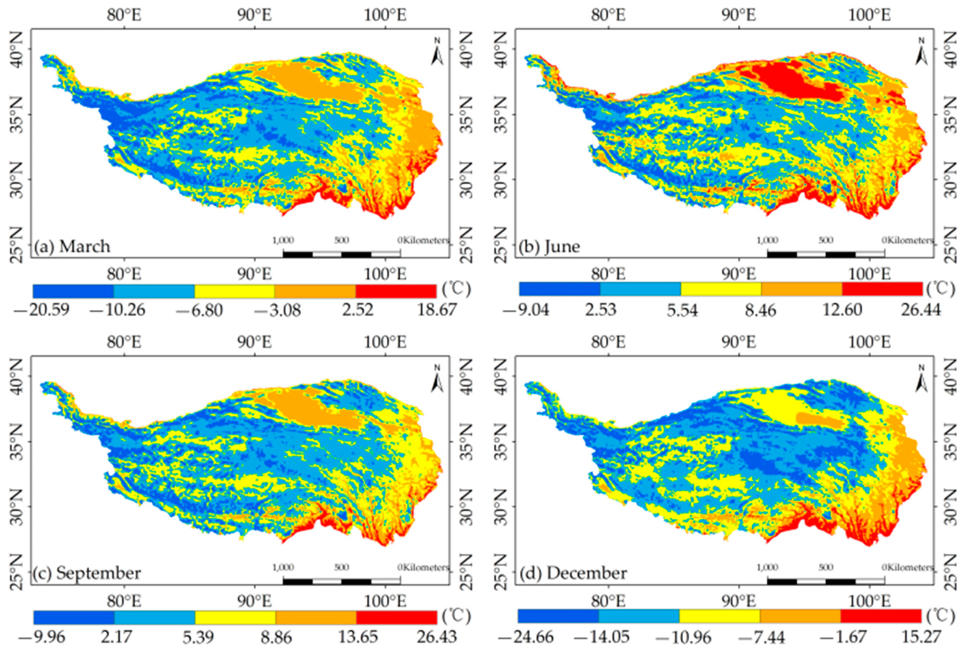
The digital elevation map (DEM) data from the QTP has a resolution of 1 arc second (Figure 1) from the digital elevation data (coverage map: viewfinderpanoramas.org). The ArcMAP 10.2software concatenates and crops the maps, before calculating relevant terrain factors included in the underlying surface impact factors [27]. Finally, the elevation range of the QTP is between 311 and 8806 m. The meteorological data were obtained from the National QTP Scientific Data Center (TPDC.ac.cn) [28]. The temporal phase of the Sentinel-1 data to determine the average temperature (Figure 2) and precipitation (Figure 3) were compared for the March (spring equinox), June (summer solstice), September (autumn equinox), and December (winter solstice) 2020 data. Figure 4 illustrates the data processing and design process of machine learning solutions.

2.3. Measured Soil Moisture Data

Measured soil moisture data were obtained from the European Space Agency Climate Change Initiative (ESA CCI). The CCI project was launched in 2020 and produces annually updated soil moisture products. All passive datasets were processed using the LPRMv7.1 algorithm. Here, the measured data were from the CII-Soil Moisture-fv06.1 version, with a spatial resolution of 0.25 × 0.25 m [29,30,31]. Similarly, the soil moisture monitoring data from 20 March, 21 June, 20 September, and 21 December 2020 were taken from the ESA CCI-Soil Moisture dataset as reference measured data. The calculated results were compared and corrected with the constructed inversion model.

2.4. Semi-Empirical Model for Inverting Soil Moisture

Considering the plateau climate and permafrost characteristics of the QTP, the vegetation coverage is composed primarily of low vegetation types, such as meadows and grasslands. The biological community accounts for about 55.6% of the total area, while climate warming and human activities have gradually reduced the grasslands by 38.8%. This makes soil moisture inversion convenient in regions based on microwave remote sensing semi-empirical models [32,33]. The Sentinel-1 GRD data include VV and VH polarizations, which are sensitive to moisture observations and have the best detection effect. Moreover, using the microwave polarization difference index (MPDI) simulates and removes the impact of vegetation canopy moisture from soil moisture retrieval. The calculation formula for the MPDI is:
M P D I = σ V V 0 σ V H 0 1 2 σ V V 0 + σ V H 0  
where σ V V 0 and σ V H 0   are the decibelization radar backscatter coefficients for VV and VH polarization modes, respectively.
The influence of surface roughness must be removed when calculating soil moisture based on semi-empirical models due to the rich surface radiation information recorded in SAR polarization data. Therefore, the lookup table method in AIEM provides calculation formula parameters [34]. Formulas can be organized into exponential patterns as:
σ V = 10 A · σ V V 0 + B · σ V H 0 + C  
where A, B, and C are the coefficients of the two radar polarization methods, with neither A nor B being 0, and σ V is the simulated surface roughness.
The semi-empirical model based on the radar backscatter coefficient has been fully developed for inverting soil moisture using corrections for a large amount of empirical data [35]. Semi-empirical models can consider the accuracy and applicability of model inversion with multiple factors and different scales under flexible conditions. Therefore, a semi-empirical model was selected as the basis for the experimental fitting, as related to various factors to invert soil moisture. The semi-empirical model constructed based on the radar-scattering coefficient and different factors is:
σ s o i l = f σ V V 0 , σ V H 0 + y + g θ  
where σ s o i l is the soil moisture index, and f( σ V V 0 , σ V H 0 ) is a function related to the radar backscatter coefficient and reserves the radar backscatter coefficient features for improved semi-empirical models. The y is a fitting model for various factors involved in inversion, and g ( θ ) is a parameter related to influencing factors and is usually a constant.
This article has two main categories: terrain and climate factors. Terrain factors include the slope gradient, aspect, and angle. The slope gradient and aspect are included in the selected terrain factors as model inputs, as they are essential parameters for analyzing the terrain and topography of the region. Considering that the elevation and slope aspect of the QTP affect surface lighting (impact ice and snow cover and melting in extreme climates, such as heavy snowfall and sudden temperature drops, and are related to glacial erosion landforms), the slope angle reflects the relationship between the slope gradient and the length from another perspective. Therefore, the slope angle was added as a terrain factor to emphasize these effects. Climate factors include the temperature and precipitation. The design fitting models are related to the expressions shown in Table 1.

2.5. Neural Network Learning Scheme

An ANN simulates the working model of human brain neurons by constructing mathematical models, repeated training, and learning known information to establish different network models to process information and simulate relationships between input and output values [36,37]. As ANN process data only know non-scalar parameters between the input and output values, they are commonly used for systematic analyses of large-scale complex structures with ambiguous data [38]. Soil moisture is influenced by multiple factors, such as climate, surface cover, human activities, and soil characteristics. Using ANN regression analyses to determine correlations between values ensures the accuracy and effectiveness [30,39,40]. The ArcGIS software was used to uniformly extract samples, with terrain features, temperature, and precipitation information from the same sample points. The ANN regression analysis then verifies the impact significance of various factors on the soil moisture values at different times. The degree of normalization importance was then determined to screen and construct model elements.

2.6. Analyzing Model Accuracy Based on Decision Tree

The decision tree is a tree-like data-mining algorithm. It is a supervised learning process that finds rules and adapts to them through nodes. This approach is divided into classification and regression trees [41]. The core technology of the decision tree for data processing is to establish an algorithm using a training sample set and then optimize it using a test sample set to classify and predict variable relationships [42]. Common decision tree algorithms include the ID3 and C4.5 [43], the PUBLIC algorithm, and the Chi-squared Automatic Interaction Detector (CHAID) [44].
Each algorithm continuously optimizes and improves its learning ability based on the growth and pruning model of decision trees, but the data attribute requirements vary. The input parameters and attribute characteristics of the fit pattern built for the model under the same phase are similar but significantly differ in various time phases. The CHAID efficiently completes data-mining tasks while processing multiple highly correlated data with redundant linear and nonlinear elements and overcoming the deficiencies of traditional parameter testing methods to compensate for missing data. Therefore, CHAID was selected to solve the problem of over-approximating the data analysis [45,46].

3. Results

3.1. Climatic Characteristics

Figure 2 shows that the average temperature in the southern region of the QTP is generally lower in March and December, while it gradually increases from June and September. Combined with regional elevation data analysis, plain areas with average elevations less than 3000 m in the northeast have higher temperatures throughout the year. The average temperature in June from the sample data was highest at 26.44 °C, with a minimum temperature of −9.04 °C. Areas with lower elevations than average correspond to greater average temperatures. The average temperature fluctuations are more pronounced in the southern and eastern edges due to significant changes in the slope gradient. The average temperature is relatively stable in flat areas with a slope gradient of 0.
Combining the precipitation data in Figure 3 with the regional DEM data indicated that the edge areas (holding an elevation below 2800 m and southern and southeastern parts of the plateau) generally have higher precipitation. The overall annual precipitation is greater in the southeast but lower in the northwest inland region. The annual precipitation is relatively stable in the central and northern regions with smooth slope gradients, where the extreme range of precipitation change is about 2.54 mm. In southern regions with significant slope gradients, this reaches 13.02 mm. In the northwest region with higher elevations and sunny slopes with lower gradients, the average precipitation is large, but with a small range of 2.10 mm.
The comparative analysis suggests that the annual average temperature and precipitation changes are relatively small in the northern plain and southern edge areas of the QTP, where the average elevation is below 3000 m. The annual temperature is generally higher in edge areas with lower elevations. The monthly average precipitation is higher in areas with significant slope gradient changes. These further prove the importance of the mutual influence and interaction between the terrain and climate in the QTP.

3.2. Significance of Factor Impact

This step is based on basic data using the ANN method to preliminarily screen out factors with significant impacts. A total of 176 random sample points were selected in the study area and randomly divided into the training dataset (123 points, approximately 70% of the samples) and validation dataset (53 points, approximately 30% of the samples). Subsequently, an S-type function and optimization algorithm with gradient descent activated the response between various data. The initial learning rate of 0.6 ensures the calculated interval offset does not exceed 0.5, excluding missing values and significant deviations. Thus, the maximum number of iterations for machine learning is 1000.
Correlations between each factor and the measured soil moisture were analyzed to obtain the statistical results shown in Table 2. The selected factors were all correlated with the measured soil moisture. The temperature in September and elevation in December were significantly correlated with soil moisture at the 0.01 level, making them the most significant influencing factors. The other factors were correlated at the 0.05 level.
Although the significant effects of various factors on soil moisture in different seasons vary, some contractions with soil moisture exist, and their importance cannot be ignored. These can be used as input parameters to verify the factor influence mechanisms. In addition, many factors dictate the soil moisture, such as the vegetation moisture content-related indices [47,48,49], terrain and geomorphic factors [3,50], and other climate-related factors [51,52]. These factors impact soil moisture with varying degrees and mechanisms.

3.3. Ensuring Model Input Parameters

The results of the significance analysis of each factor were summarized. Two primary categories (terrain and climate factors) were considered within the parameters for the normalization importance analysis. The terrain factors include the elevation, slope gradient, slope aspect, and slope angle, while the climate factors include the temperature and precipitation, yielding six factors in total. The existence of correlations between similar factors with significant impacts makes it necessary to conduct normalization fitting to determine the importance of each factor on the soil moisture more directly, optimize the model parameters, and reduce redundancy in model data construction to emphasize the correlation between each factor and the final model.
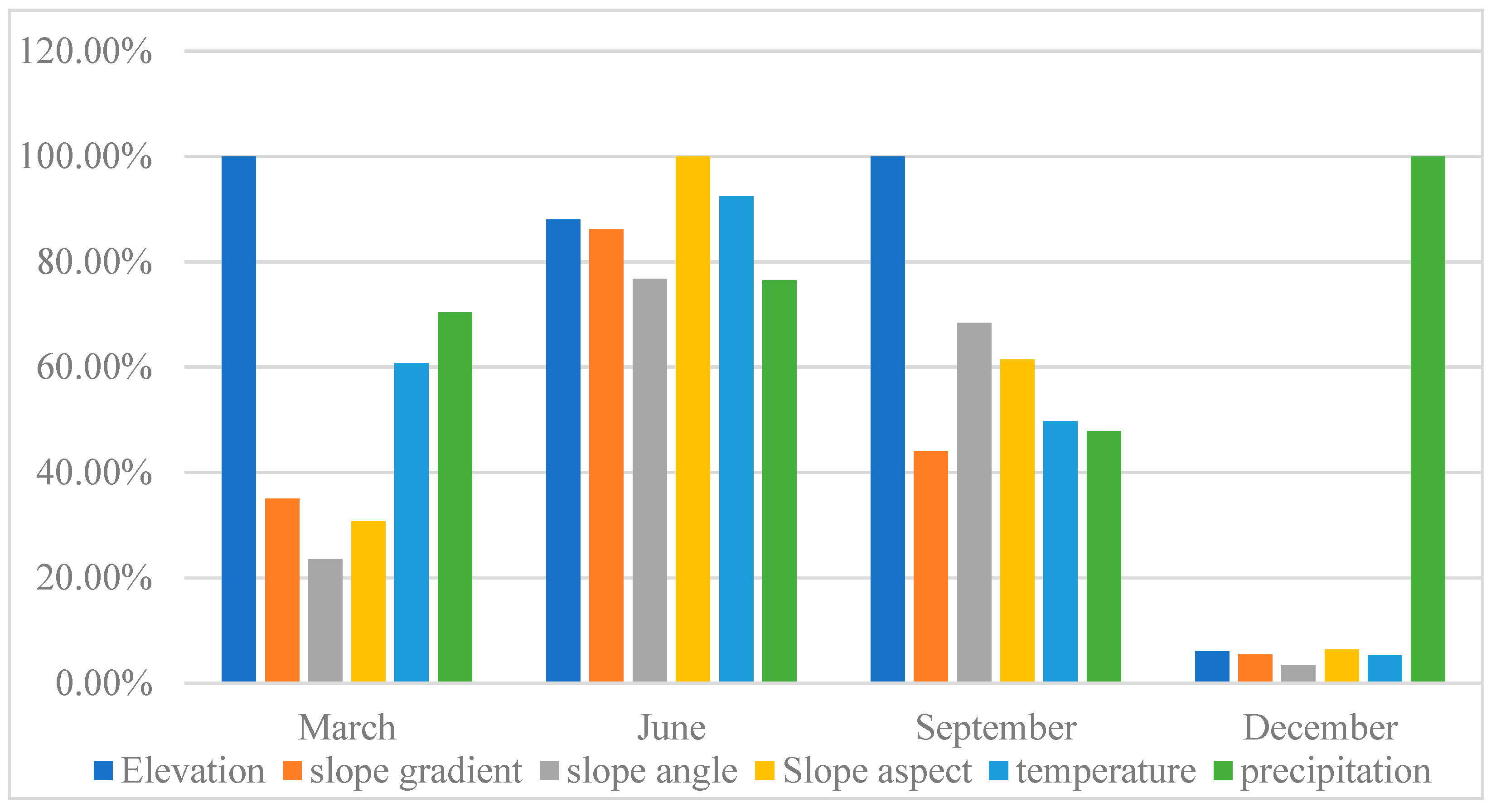
Due to the specific high-altitude climate of the QTP, changes in each factor significantly impact the environment within the region [27]. Therefore, the impact of the climate background in different seasons on soil moisture retrieval cannot be ignored. It is necessary to verify the normalized importance of each factor in soil moisture retrieval based on the seasonal phase. The statistical results are shown in Figure 5.
Figure 5 indicates that the factor with the greatest normalized impact on the soil moisture in the QTP in March and September is the elevation, with precipitation having a secondary effect in March and slope angle in September. In June, the slope aspect has the most influence. The elevation, slope, and temperature all impact soil moisture retrieval at that time. Concentrated precipitation along the QTP in December 2020, such as snowfall and ice melting, significantly impacts soil moisture retrieval, making the impact of climate factors in December more important. Meanwhile, the effects of elevation on the climate factor distributions in the region cannot be ignored.
Terrain is the most important factor affecting soil moisture in the QTP. In addition to extreme precipitation, temperature is one of the main factors affecting soil moisture. This is due to the high elevation characteristics over the QTP, affecting surface evapotranspiration in June and September when the temperatures are generally high, significantly impacting the soil moisture index. An inverse trigonometric function relationship exists between the slope gradient and the slope angle, which restricts the soil moisture. The division of the slope aspect is more objective and primarily related to the direction. Therefore, the influence of the slope aspect peaks in June when the insolation is greatest. Correspondingly, the influence of various terrain factors is small in December when the night is dominant.

3.4. Establishing an Optimization Model Based on Machine Learning Methods

The input model factors were screened using the temporal background of the data based on the normalized importance analysis results of each factor. The constructed ANN learning scheme used the semi-empirical model for soil moisture inversion.
Considering the importance of normalized soil moisture in March, the factors, in order of influence, are elevation, precipitation, and temperature. We established three sets of input parameters to calculate the synergistic effects of elevation and precipitation, elevation and temperature, and elevation, precipitation, and temperature on soil moisture retrieval. Therefore, 15 experiments were designed based on the influence model of the factor fitting. With the upward temperature trend in June, the normalized factors, in order of influence, are the slope aspect, temperature, elevation, and other terrain factors. There are also correlations between terrain factors. Therefore, we selected the slope aspect, temperature, and elevation as the primary input parameters and designed three sets of experiments. In September, the normalization factors, in order of importance on the soil moisture, are elevation, slope angle, and slope aspect. The normalized impacts from climate factors, temperature, and precipitation were each less than 50%. As there were no quantifiable synergistic effects between the slope angle and aspect, only two sets of experiments were designed. The elevation and slope angle were the input factors for Experiments 31–35, and elevation and aspect were the input factors for Experiments 36–40. In December, the severe snow cover and extremely cold climate in the QTP caused precipitation to be the most influential normalized factor, with terrain factors still greatly affecting snow cover on the plateau. Therefore, it is necessary to consider the impact of precipitation with the foundation of terrain factors and conduct a set of experiments.
A total of 45 experiments were considered by combining the 5 methods of fitting different factors using the semi-empirical model of microwave remote sensing, as shown in Table 3. Verification determined the model accuracy. Each experiment individually verified the coefficients of the parameters in the model. The operation ended when the cumulative accuracy increase in the calculations was less than 0.001 up to a maximum of 1000 iterations.

3.5. Model Accuracy Verification

Pearson correlation analysis was used on the simulated and measured values for the 45 experiments to verify the accuracy of numerical inversion. The impact of various factors on soil moisture inversion was explored using the decision tree CHAID method to analyze the model accuracy [53]. The CHAID algorithm has a maximum number of iterations of 100, and the results are shown in Table 4.
The statistical results in Table 4 indicate that the model with the Pearson index became anomalous (such as negative values and 1). Accuracies less than 50.0% are incorrect, so they were eliminated. In the corresponding experiments in Table 3 and Table 4, the eliminated experimental models are highlighted in red, while the preferred experimental models are bolded. The model elimination and optimization rates were 17.8% and 33.3%, respectively. Thus, the experimental input parameters were appropriate, and the success rate of the constructed model was generally high. The monthly analysis is given as follows:
  • In March, there were 15 experiments to calculate the synergistic effects of statistical elevation and precipitation, elevation and temperature, and elevation, precipitation, and temperature on the soil moisture retrieval. The experimental data showed satisfactory results, with a 0% model elimination rate. Experiments 1, 5, 10, 11, and 12 were the best models based on the Pearson index for simulated soil moisture and the designed model accuracy. The model accuracy in Experiment 11 was the highest at 95.7%. The Pearson index was 0.389, reaching the inversion accuracy requirements. Although the model accuracy in Experiment 1 was 85.7%, lower than Experiment 11, the Pearson index was 0.408, significantly higher than the inversion accuracy of the model in Experiment 11. This reaches the requirements of high accuracy and model inversion. The model accuracy in Experiment 5 was also high at 88.0%, with a Pearson index of 0.413, indicating a good model accuracy. Although the model accuracies in Experiments 10 and 12 were high at ≥80.0%, the Pearson index inverted by the model was relatively unstable and had wide variability.
  • In June, three sets of experiments were designed for soil moisture in the QTP. The rates of elimination and experimental models were both high, indicating that these input parameters cannot generally reach the stability requirements of the inversion model. After comparison, the optimal fitting models were Experiments 20, 22, 25, and 29. Only the model accuracy and Pearson index of Experiment 29 were both high, with values of 60% and 0.459, respectively, reaching the model requirements. The model accuracy of Experiment 22 was 65.2%, and the Pearson index was 0.424, indicating good results. However, the Pearson index of Experiment 20 was 0.273, and that of Experiment 25 was 0.116, significantly lower than the other optimal models.
  • In September, two sets of experiments were designed for soil moisture in the QTP, with satisfactory results. The model elimination rate was 10%, and Experiments 31, 35, and 40 were selected as optimal models due to their higher Pearson index and model accuracy. The accuracy and Pearson index of Experiment 31 were 79.2% and 0.592, respectively, indicating good results. The model accuracy and Pearson index for fitting soil moisture in Experiments 35 and 40 were similar, but the model accuracies were lower than in Experiment 31.
  • In December, five experiments were designed for soil moisture in the QTP. The elimination rate of the model was relatively low, at 20%. The model in Experiment 42 had the highest accuracy of 70.4%, and the Pearson index was 0.445, indicating that the inversion accuracy of the model was sufficient. Experiment 41 had the highest Pearson index of 0.480.

4. Discussion

4.1. Seasonal Characteristics of Factor Influence

The QTP has abundant frozen soil resources, with most being permanently frozen soil. However, soil moisture is directly affected by global warming and seasonal lake thawing, resulting in strong seasonal soil moisture characteristics [54]. It is necessary to screen these factors to improve the model inversion accuracy and retrieve soil moisture based on different seasonal backgrounds.
First, high elevation is the stronger feature of the QTP, as it affects surface evapotranspiration and directly impacts soil moisture. The other terrain factors related to elevation, such as the slope gradient, aspect, and angle, can affect soil moisture directly or indirectly. Among them, the slope aspect affects the surface by altering the duration of continuous sunlight exposure. The slope angle reflects the intensity of surface runoff, and the slope gradient reflects the synergistic effect of sunlight exposure and surface runoff. According to the normalized statistical results for the influence of the factors in Figure 5, the overall impact of terrain factors is relatively high in summer (June) with sufficient sunlight, and the normalized impact of the slope aspect on soil moisture is the largest, at 100%. This is similar to the conclusion drawn by Penna et al. [55]. The overall impact of terrain factors is relatively low in winter (December) when sunlight is the scarcest. In spring (March) and autumn (September) when the sunlight duration is balanced, elevation is the main influencing factor, with an impact effect reaching 100%.
The impact of climate factors on the model more directly reflects seasonal changes in the region. The selected climate factors include temperature and precipitation. Based on the analysis of the temperature spatial distribution map in Figure 2 and the experimental results in Table 4, the model has a high elimination rate and low inversion accuracy in summer (June), with an uneven spatial temperature distribution. Thus, the temperature is not a suitable input factor for soil moisture inversion at that time. Only inputting terrain factors into the inversion model seems to correct this phenomenon. Due to snow cover and permafrost in the QTP during winter (December), precipitation has the greatest normalization effect on soil moisture, reaching 100%. The accuracy of the model inversion also met the requirements.
Thus, there are clear seasonal correlations between various factors affecting soil moisture in the QTP. Selecting different parameters based on seasons as the inputs into the soil inversion model more effectively ensures its accuracy.

4.2. Optimization

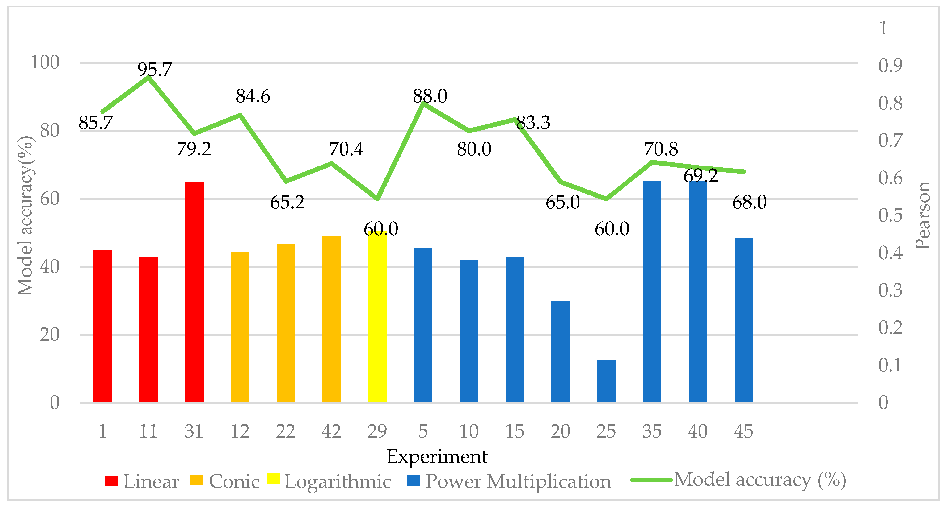
The results were further statistically analyzed using the preferred model in Table 4 to understand the impacts of different fitting mechanisms on the semi-empirical model for soil moisture inversion better and more directly. The statistical results are shown in Figure 6.
First, the accuracy of the linear fit model was generally high, along with the Pearson index of the power fit model. However, the Pearson indexes of Experiments 20 and 25 in the power fit model were low at 0.273 and 0.116, indicating strict conditions for model use. Second, in the linear fitting model, the accuracy in Experiment 11 reached 95.7%, and that in Experiment 1 reached 85.7%, significantly improving the inversion accuracy compared to traditional models [56,57]. Moreover, the accuracy and Pearson index of the simulated values in Experiment 31 were both high, at 79.2% and 0.592, respectively, indicating that the linear fit not only ensures the accuracy of the inversion values but also meets the requirements of universal inversion. With power fit models, Experiments 35 and 40 had higher simulated Pearson indexes but lower accuracy rates of 70.8% and 69.2%, respectively. In contrast, Experiments 5, 10, and 15 had lower Pearson indexes but higher accuracies of 88.0%, 80.0%, and 83.3%, respectively.
Finally, a comprehensive comparison of the experimental results and numerical values suggested that there is usually a restricted relationship between the model accuracy and the Pearson index of the simulated values, making it difficult to simultaneously achieve a good numerical relationship. This effect is strongest in the power product fit models. Of all the experimental models, only Experiment 31 achieved a high model accuracy and Pearson index for simulated values. The parameter model for soil moisture inversion was a linear fit composed of the elevation and slope angles. The accuracy of the model was 79.2%, and the Pearson index was 0.592.
The input factors from various experimental models in the ANN learning scheme showed that the most suitable factors for constructing fitting models were the elevation and precipitation in March, slope aspect and temperature in June, elevation and slope angle in September, and elevation, temperature, and precipitation in December. In addition, the fitting method with the greatest optimization rate in the model was power multiplication fitting. However, the Pearson index inverted by the model was relatively unstable. The Pearson index inverted by the model in Experiment 25 was only 0.116, but it reached 0.594 in Experiment 40. Thus, the power multiplication fitting model has high requirements for the sample data. However, the linear fit model ensures the inversion accuracy while effectively reaching the universal applicability requirements.

5. Conclusions

This article used Sentinel-1 SAR data and was based on the semi-empirical model of soil moisture inversion. Taking the QTP region as an example, an ANN learning scheme was designed to analyze the significance of factors affecting soil moisture inversion. Through normalization, factors were selected and fitted into the model. After that, the decision tree algorithm was used to analyze the model accuracy and Pearson index of the simulated values. The combination of factors and the fitting model were compared to exclude factors, screen the optimal fitting model, and obtain experience in model optimization.
Comparative verification of data results showed that the main factor affecting soil moisture retrieval in the QTP was terrain, with an impact that conformed to a linear fit model. At the same time, the impact of climate factors cannot be ignored. For example, in the uneven spatial temperature distribution on the QTP during the summer solstice, temperature was involved in soil moisture retrieval, and this can reduce the stability of the model inversion results.
With the development of remote sensing technology, more precise continuous ground observations have progressed, and more factors are conducive to improving the accuracy of soil moisture inversion models. The model optimization approach proposed in this article can be combined with other factors and fitting methods, with comparisons and verifications of the accuracy with field-measured data to be widely used to improve soil moisture inversion models in other regions. This could provide higher-precision soil moisture inversion results and more effective means for liberating human, material, and financial resources for soil quality monitoring.

Author Contributions

Conceptualization, J.Y. and L.Z.; methodology, Q.D. and J.Y.; formal analysis, Q.D. and J.Y.; resources, Z.S. and Q.C.; data curation, G.S. and F.D.; writing—original draft preparation, Q.D. and J.Y.; writing—review and editing, Q.D., J.Y. and L.Z. All authors have read and agreed to the published version of the manuscript.

Funding

This research was funded by the Key R&D Plan of Shandong Province (Soft Science Project, Grant Number 2022RZB07056). Grateful appreciation is expressed for the support.

Data Availability Statement

The data presented in this study are available upon request from the corresponding author.

Acknowledgments

The authors would like to thank the Copernicus program of the European Space Agency (ESA) for providing Sentinel-1A and soil moisture data, and Jonathan de Ferranti for arranging the digital elevation data. The data for eliminating atmospheric error were provided by the Generic Atmospheric Correction Online Service (GACOS). Many thanks to the editor and anonymous reviewers for their valuable advice, which improved the paper.

Conflicts of Interest

The authors declare no conflict of interest.

References

  1. Shellito, P.J.; Small, E.E.; Livneh, B. Controls on surface soil drying rates observed by SMAP and simulated by the Noah land surface model. Hydrol. Earth Syst. Sci. 2018, 22, 1649–1663. [Google Scholar] [CrossRef] [Green Version]
  2. Rodriguez-Iturbe, I.; Chen, Z.; Rinaldo, A. On the fractal structure of soil moisture fields. Adv. Water Resour. 2021, 147, 103826. [Google Scholar] [CrossRef]
  3. Rasheed, M.W.; Tang, J.; Sarwar, A.; Shah, S.; Saddique, N.; Khan, M.U.; Imran Khan, M.; Nawaz, S.; Shamshiri, R.R.; Aziz, M.; et al. Soil Moisture Measuring Techniques and Factors Affecting the Moisture Dynamics: A Comprehensive Review. Sustainability 2022, 14, 11538. [Google Scholar] [CrossRef]
  4. Shi, J.; Jiang, L.; Zhang, L.; Chen, K.S.; Wigneron, J.P.; Chanzy, A.; Jackson, T.J. Physically Based Estimation of Bare-Surface Soil Moisture With the Passive Radiometers. IEEE Trans. Geosci. Remote Sens. 2006, 44, 3145–3153. [Google Scholar] [CrossRef]
  5. Zhu, W.; Wang, Y.; Jia, S. A remote sensing-based method for daily evapotranspiration mapping and partitioning in a poorly gauged basin with arid ecosystems in the Qinghai-Tibet Plateau. J. Hydrol. 2023, 616, 128807. [Google Scholar] [CrossRef]
  6. Rafiei Sardooi, E.; Azareh, A.; Mesbahzade, T.; Sardoo, F.; Parteli, E.; Pradhan, B. A hybrid model using data mining and multi-criteria decision-making methods for landslide risk mapping at Golestan Province, Iran. Environ. Earth Sci. 2021, 80, 487. [Google Scholar] [CrossRef]
  7. Zhao, Z.; Fu, R.; Liu, J.; Dai, L.; Guo, X.W.; Du, Y.; Hu, Z.; Cao, G. Response of Seasonally Frozen Ground to Climate Changes in the Northeastern Qinghai-Tibet Plateau. Front. Environ. Sci. 2022, 10, 912209. [Google Scholar] [CrossRef]
  8. Han, Y.; Bai, X.; Shao, W.; Wang, J. Retrieval of Soil Moisture by Integrating Sentinel-1A and MODIS Data over Agricultural Fields. Water 2020, 12, 1726. [Google Scholar] [CrossRef]
  9. Bai, X.; Zeng, J.; Chen, K.S.; Li, Z.; Zeng, Y.; Wen, J.; Wang, X.; Dong, X.; Su, Z. Parameter Optimization of a Discrete Scattering Model by Integration of Global Sensitivity Analysis Using SMAP Active and Passive Observations. IEEE Trans. Geosci. Remote Sens. 2019, 57, 1084–1099. [Google Scholar] [CrossRef]
  10. Bai, X.; He, B.; Li, X.; Zeng, J.; Wang, X.; Wang, Z.; Zeng, Y.; Su, B. First Assessment of Sentinel-1A Data for Surface Soil Moisture Estimations Using a Coupled Water Cloud Model and Advanced Integral Equation Model over the Tibetan Plateau. Remote Sens. 2017, 9, 714. [Google Scholar] [CrossRef] [Green Version]
  11. Dubois, P.C.; Zyl, J.v.; Engman, T. Measuring soil moisture with imaging radars. IEEE Trans. Geosci. Remote Sens. 1995, 33, 915–926. [Google Scholar] [CrossRef] [Green Version]
  12. Oh, Y.; Sarabandi, K.; Ulaby, F.T. An empirical model and an inversion technique for radar scattering from bare soil surfaces. IEEE Trans. Geosci. Remote Sens. 1992, 30, 370–381. [Google Scholar] [CrossRef]
  13. Fung, A.K.; Li, Z.; Chen, K.S. Backscattering from a randomly rough dielectric surface. IEEE Trans. Geosci. Remote Sens. 1992, 30, 356–369. [Google Scholar] [CrossRef]
  14. Zeng, J.; Chen, K.S.; Bi, H.; Zhao, T.; Yang, X. A Comprehensive Analysis of Rough Soil Surface Scattering and Emission Predicted by AIEM with Comparison to Numerical Simulations and Experimental Measurements. IEEE Trans. Geosci. Remote Sens. 2017, 55, 1696–1708. [Google Scholar] [CrossRef]
  15. Popkov, Y.S. Randomization and Entropy in Machine Learning and Data Processing. Dokl. Math. 2022, 105, 135–157. [Google Scholar] [CrossRef]
  16. Mauri, P.V.; Parra, L.; Mostaza-Colado, D.; Garcia, L.; Lloret, J.; Marin, J.F. The Combined Use of Remote Sensing and Wireless Sensor Network to Estimate Soil Moisture in Golf Course. Appl. Sci. 2021, 11, 11769. [Google Scholar] [CrossRef]
  17. Cordeiro, A.S.; Santos, S.R.d.; Moreira, F.B.; Santos, P.C.; Carro, L.; Alves, M.A.Z. Efficient Machine Learning execution with Near-Data Processing. Microprocess. Microsyst. 2022, 90, 104435. [Google Scholar] [CrossRef]
  18. Notarnicola, C.; Angiulli, M.; Posa, F. Soil moisture retrieval from remotely sensed data: Neural network approach versus Bayesian method. IEEE Trans. Geosci. Remote Sens. 2008, 46, 547–557. [Google Scholar] [CrossRef]
  19. Baghdadi, N.; Cresson, R.; El Hajj, M.; Ludwig, R.; La Jeunesse, I. Estimation of soil parameters over bare agriculture areas from C-band polarimetric SAR data using neural networks. Hydrol. Earth Syst. Sci. 2012, 16, 1607–1621. [Google Scholar] [CrossRef] [Green Version]
  20. Quinlan, J.R. Induction of decision trees. Mach. Learn. 1986, 1, 81–106. [Google Scholar] [CrossRef] [Green Version]
  21. Breiman, L. Random Forests. Mach. Learn. 2001, 45, 5–32. [Google Scholar] [CrossRef] [Green Version]
  22. Pasolli, L.; Notarnicola, C.; Bruzzone, L.; Bertoldi, G.; Chiesa, S.D.; Niedrist, G.; Tappeiner, U.; Zebisch, M. Polarimetric RADARSAT-2 imagery for soil moisture retrieval in alpine areas. Can. J. Remote Sens. 2011, 37, 535–547. [Google Scholar] [CrossRef]
  23. Hunt, E.B. Concept Learning: An Information Processing Problem; John Wiley & Sons: Hoboken, NJ, USA, 1974. [Google Scholar]
  24. Cordella, L.P.; Foggia, P.; Sansone, C.; Vento, M. Learning structural shape descriptions from examples. Pattern Recognit. Lett. 2002, 23, 1427–1437. [Google Scholar] [CrossRef]
  25. Yuan, J.; Xiang, S.; Xia, J.; Yu, L.; Liu, S. Evaluation of Sampling Methods for Scatterplots. IEEE Trans. Vis. Comput. Graph. 2021, 27, 1720–1730. [Google Scholar] [CrossRef] [PubMed]
  26. Shi, N.; Naudiyal, N.; Wang, J.; Gaire, N.P.; Wu, Y.; Wei, Y.; He, J.; Wang, C. Assessing the Impact of Climate Change on Potential Distribution of Meconopsis punicea and Its Influence on Ecosystem Services Supply in the Southeastern Margin of Qinghai-Tibet Plateau. Front. Plant Sci. 2021, 12, 830119. [Google Scholar] [CrossRef]
  27. Zhou, C.P. The Spatial Dataset of Climate on the Tibetan Plateau (1961–2020). A Big Earth Data Platform for Three Poles. 2014. Available online: https://data.tpdc.ac.cn/en/data/ca3ce8da-fbfd-4d3c-a4ca-7a821c5f7203 (accessed on 8 July 2023).
  28. Shen, X.; An, R.; Quaye-Ballard, J.A.; Zhang, L.; Wang, Z. Evaluation of the European Space Agency Climate Change Initiative Soil Moisture Product over China Using Variance Reduction Factor. JAWRA J. Am. Water Resour. Assoc. 2016, 52, 1524–1535. [Google Scholar] [CrossRef]
  29. Zhang, K.; Wang, Q.; Chao, L.; Ye, J.; Li, Z.; Yu, Z.; Yang, T.; Ju, Q. Ground observation-based analysis of soil moisture spatiotemporal variability across a humid to semi-humid transitional zone in China. J. Hydrol. 2019, 574, 903–914. [Google Scholar] [CrossRef]
  30. Zhang, L.; Liu, Y.; Ren, L.; Teuling, A.J.; Zhang, X.; Jiang, S.; Yang, X.; Wei, L.; Zhong, F.; Zheng, L. Reconstruction of ESA CCI satellite-derived soil moisture using an artificial neural network technology. Sci. Total Environ. 2021, 782, 146602. [Google Scholar] [CrossRef]
  31. Pan, T.; Zou, X.; Liu, Y.; Wu, S.; He, G. Contributions of climatic and non-climatic drivers to grassland variations on the Tibetan Plateau. Ecol. Eng. 2017, 108, 307–317. [Google Scholar] [CrossRef]
  32. Wang, X.; Yi, S.; Wu, Q.; Yang, K.; Ding, Y. The role of permafrost and soil water in distribution of alpine grassland and its NDVI dynamics on the Qinghai-Tibetan Plateau. Glob. Planet. Chang. 2016, 147, 40–53. [Google Scholar] [CrossRef]
  33. Bindlish, R.; Barros, A.P. Multifrequency Soil Moisture Inversion from SAR Measurements with the Use of IEM. Remote Sens. Environ. 2000, 71, 67–88. [Google Scholar] [CrossRef]
  34. Rawat, K.; Sehgal, V.; Pradhan, S.; Ray, S. Semi-empirical model for retrieval of soil moisture using RISAT-1 C-Band SAR data over a sub-tropical semi-arid area of Rewari district, Haryana (India). J. Earth Syst. Sci. 2018, 127, 18. [Google Scholar] [CrossRef] [Green Version]
  35. Hornik, K.; Stinchcombe, M.; White, H. Multilayer feedforward networks are universal approximators. Neural Netw. 1989, 2, 359–366. [Google Scholar] [CrossRef]
  36. Shi, C.; Cui, J.; Liu, X.; Zhang, Y.; Qin, N.; Luo, Y. Application of artificial neural network to predict the change of inosine monophosphate for lightly salted silver carp (hypophthalmichthys molitrix) during thermal treatment and storage. J. Food Process. Preserv. 2017, 41, e13246. [Google Scholar] [CrossRef]
  37. Banerjee, A. Learning Precise Spike Train–to–Spike Train Transformations in Multilayer Feedforward Neuronal Networks. Neural Comput. 2016, 28, 826–848. [Google Scholar] [CrossRef] [Green Version]
  38. He, Z.; Zhao, W.; Liu, H.; Chang, X. The response of soil moisture to rainfall event size in subalpine grassland and meadows in a semi-arid mountain range: A case study in northwestern China’s Qilian Mountains. J. Hydrol. 2012, 420–421, 183–190. [Google Scholar] [CrossRef]
  39. Mo, K.; Chen, Q.; Chen, C.; Zhang, J.; Wang, L.; Bao, Z. Spatiotemporal variation of correlation between vegetation cover and precipitation in an arid mountain-oasis river basin in northwest China. J. Hydrol. 2019, 574, 138–147. [Google Scholar] [CrossRef]
  40. Kizyakov, A.I.; Wetterich, S.; Günther, F.; Opel, T.; Jongejans, L.L.; Courtin, J.; Meyer, H.; Shepelev, A.G.; Syromyatnikov, I.I.; Fedorov, A.N.; et al. Landforms and degradation pattern of the Batagay thaw slump, Northeastern Siberia. Geomorphology 2023, 420, 108501. [Google Scholar] [CrossRef]
  41. Nguyen, V.-N.; Yariyan, P.; Amiri, M.; Dang Tran, A.; Pham, T.D.; Do, M.P.; Thi Ngo, P.T.; Nhu, V.-H.; Quoc Long, N.; Tien Bui, D. A New Modeling Approach for Spatial Prediction of Flash Flood with Biogeography Optimized CHAID Tree Ensemble and Remote Sensing Data. Remote Sens. 2020, 12, 1373. [Google Scholar] [CrossRef]
  42. Salzberg, S.L. C4.5: Programs for Machine Learning by J. Ross Quinlan. Morgan Kaufmann Publishers, Inc., 1993. Mach. Learn. 1994, 16, 235–240. [Google Scholar] [CrossRef] [Green Version]
  43. Rastogi, R.; Shim, K. PUBLIC: A Decision Tree Classifier that Integrates Building and Pruning. Data Min. Knowl. Discov. 2000, 4, 315–344. [Google Scholar] [CrossRef]
  44. Luchman, J. CHAID: Stata Module to Conduct Chi-Square Automated Interaction Detection; Statistical Software Components; Boston College Department of Economics: Chestnut Hill, MA, USA, 2015. [Google Scholar]
  45. Han, J.; Kamber, M.; Pei, J. 1—Introduction. In Data Mining, 3rd ed.; Han, J., Kamber, M., Pei, J., Eds.; Morgan Kaufmann: Boston, MA, USA, 2012; pp. 1–38. [Google Scholar]
  46. Zhou, Q.; Zhu, A.X.; Yan, W.; Sun, Z. Impacts of forestland vegetation restoration on soil moisture content in humid karst region: A case study on a limestone slope. Ecol. Eng. 2022, 180, 106648. [Google Scholar] [CrossRef]
  47. Lv, J.; Zhang, R.; Tu, J.; Liao, M.; Pang, J.; Yu, B.; Li, K.; Xiang, W.; Fu, Y.; Liu, G. A GNSS-IR Method for Retrieving Soil Moisture Content from Integrated Multi-Satellite Data That Accounts for the Impact of Vegetation Moisture Content. Remote Sens. 2021, 13, 2442. [Google Scholar] [CrossRef]
  48. Feng, S.; Qiu, J.; Crow, W.T.; Mo, X.; Liu, S.; Wang, S.; Gao, L.; Wang, X.; Chen, S. Improved estimation of vegetation water content and its impact on L-band soil moisture retrieval over cropland. J. Hydrol. 2023, 617, 129015. [Google Scholar] [CrossRef]
  49. Cai, Q.; Li, E.; Chen, J.; Tao, L.; Jiang, R. Analysis on Topographic Effect of Soil Moisture in Mountainous Areas based on Landsat-8 OLI Images. J. Eng. Sci. Technol. Rev. 2020, 13, 22–29. [Google Scholar] [CrossRef]
  50. Qiu, Z.; Pennock, A.; Giri, S.; Trnka, C.; Du, X.; Wang, H. Assessing Soil Moisture Patterns Using a Soil Topographic Index in a Humid Region. Water Resour. Manag. 2017, 31, 2243–2255. [Google Scholar] [CrossRef]
  51. Lyons, D.S.; Dobrowski, S.Z.; Holden, Z.A.; Maneta, M.P.; Sala, A. Soil moisture variation drives canopy water content dynamics across the western U.S. Remote Sens. Environ. 2021, 253, 112233. [Google Scholar] [CrossRef]
  52. Tan, X.; Zhang, L.; He, C.; Zhu, Y.; Han, Z.; Li, X. Applicability of cosmic-ray neutron sensor for measuring soil moisture at the agricultural-pastoral ecotone in northwest China. Sci. China Earth Sci. 2020, 63, 1730–1744. [Google Scholar] [CrossRef]
  53. Zhao, L.; Zou, D.; Hu, G.; Wu, T.; Du, E.; Liu, G.; Xiao, Y.; Li, R.; Pang, Q.; Qiao, Y.; et al. A synthesis dataset of permafrost thermal state for the Qinghai–Tibet (Xizang) Plateau, China. Earth Syst. Sci. Data 2021, 13, 4207–4218. [Google Scholar] [CrossRef]
  54. Lu, P.; Han, J.; Li, Z.; Xu, R.; Li, R.; Hao, T.; Qiao, G. Lake outburst accelerated permafrost degradation on Qinghai-Tibet Plateau. Remote Sens. Environ. 2020, 249, 112011. [Google Scholar] [CrossRef]
  55. Penna, D.; Borga, M.; Norbiato, D.; Dalla Fontana, G. Hillslope scale soil moisture variability in a steep alpine terrain. J. Hydrol. 2009, 364, 311–327. [Google Scholar] [CrossRef]
  56. Wang, J.; Bao, Y.; Zhang, Y.; Qu, J.; Zhang, W. Soil moisture inversion using multi-polarization and multi-angle ENVISAT ASAR data in surface soils of bare area and wheat-covered area. Nongye Gongcheng Xuebao/Trans. Chin. Soc. Agric. Eng. 2010, 26, 205–210. [Google Scholar] [CrossRef]
  57. Wei, Y.; Fang, Z.; Zhang, L.; Kang, L.; Liu, X. Estimating Soil Moisture in Semi-Arid Region by Remote Sensing Based on TM Data. In Proceedings of the 2010 International Conference on Multimedia Technology, ICMT 2010, Ningbo, China, 29–31 October 2010. [Google Scholar] [CrossRef]
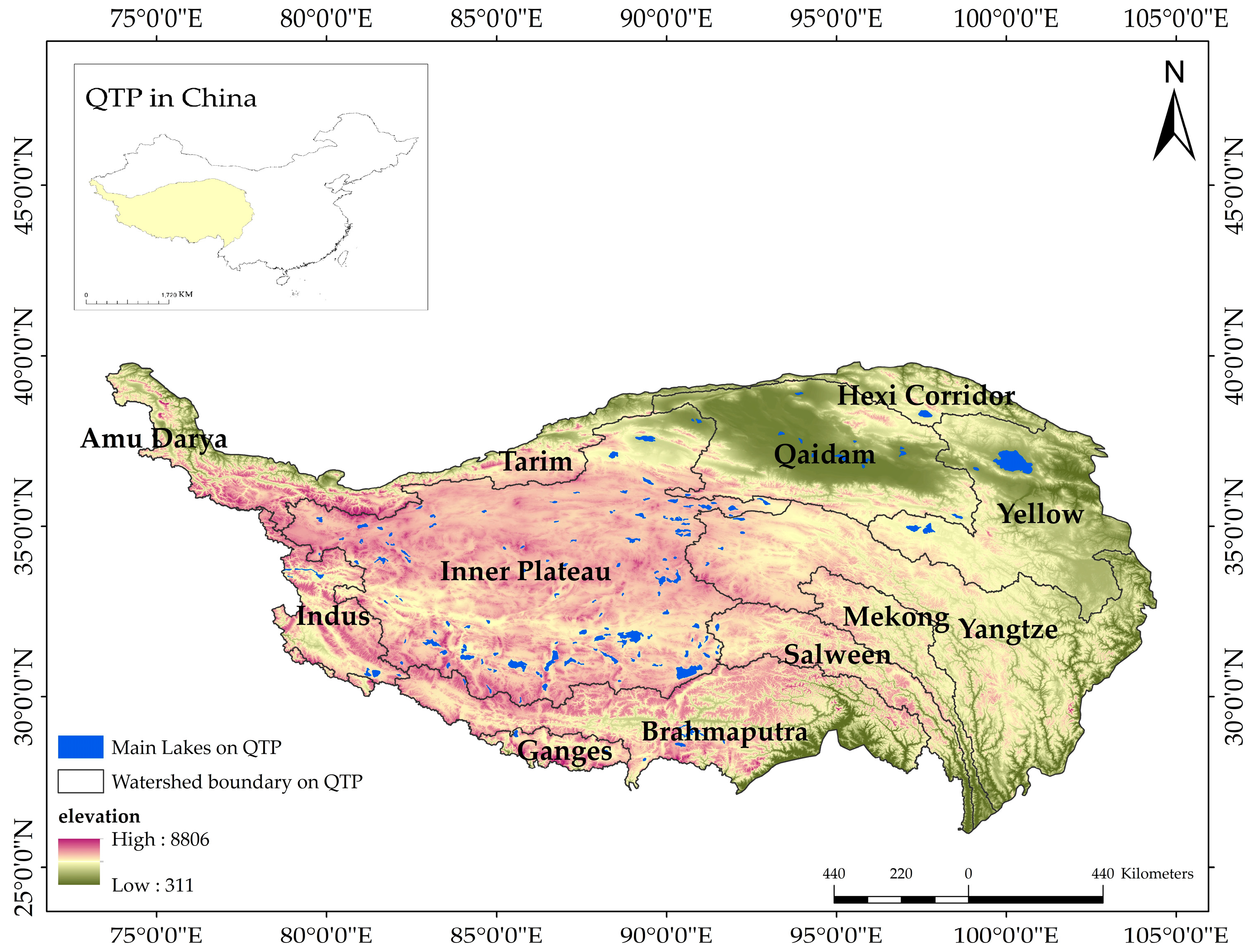
Figure 1. Geographical location of the QTP in China and the spatial distribution of the main lakes and watershed boundaries.
Water 15 02859 g001
Figure 2. Monthly average temperature distribution of the QTP in 2020.
Water 15 02859 g002
Figure 3. Monthly average rainfall distribution of the QTP in 2020.
Water 15 02859 g003
Figure 4. Flow chart steps and process of machine learning solutions.
Water 15 02859 g004
Figure 5. Normalization analysis for the importance of each factor.
Water 15 02859 g005
Figure 6. Model accuracy of each winning experiment and the Pearson index of the simulated value.
Water 15 02859 g006
Table 1. Fitting models for each factor.
Fitting ModelModel Expression
Linear y = a L x + b
Conic y = a L x 2 + b
Index y = a · e b · L ( x )
Logarithmic y = a · l n L x + b
Power Multiplication y = a · L x b + c
Note: L(x) and L(|x|) are functions related to the factors.
Table 2. Correlations between various factors and the measured soil moisture.
CorrelationInfluencing Factors
ElevationSlope GradientSlope AngleSlope AspectTemperaturePrecipitation
MonthsMarch−0.349 *−0.024−0.003−0.138 *0.193 *0.194 *
June−0.38 *−0.306 *−0.203 *−0.072 *0.154 *0.326 *
September−0.58 **−0.203 *−0.29 *0.0690.436 **0.155 *
December0.424 **−0.0960.0030.016−0.0150.244 *
Note: ** Means significantly correlated at the 0.01 level, * means significantly correlated at the 0.05 level, no * means a weak correlation.
Table 3. Parameter setting for the different ANN schemes.
MonthTestInput VariablesFitting ModelMonthTestInput VariablesFitted ModelOutput Variables
March1MPDI,  σ V ,
Elevation, and
Precipitation
LinearJune24MPDI,  σ V ,
Slope aspect, and Elevation
LogarithmicSimulate soil moisture
2Conic25Power Multiplication
3Index26MPDI,  σ V ,
Slope aspect, Temperature, and Slope gradient
Linear
4Logarithmic27Conic
5Power Multiplication28Index
6MPDI,  σ V ,
Elevation, and Temperature
Linear29Logarithmic
7Conic30Power Multiplication
8IndexSeptember31MPDI,  σ V ,
Elevation, and
Slope angle
Linear
9Logarithmic32Conic
10Power Multiplication33Index
11MPDI,  σ V ,
Elevation,
Precipitation, and Temperature
Linear34Logarithmic
12Conic35Power Multiplication
13Index36MPDI,  σ V ,
Elevation, and
Slope aspect
Linear
14Logarithmic37Conic
15Power Multiplication38Index
June16MPDI,  σ V , Slope aspect, and TemperatureLiner39Logarithmic
17Conics40Power Multiplication
18IndexDecember41MPDI,  σ V ,
Precipitation,
Temperature,
and Elevation
Linear
19Logarithmic42Conic
20Power Multiplication43Index
21MPDI,  σ V , Slope aspect, and ElevationLinear44Logarithmic
22Conic45Power Multiplication
23Index
Table 4. Statistical results of the Pearson index and model accuracy for each model.
MonthTestPearsonAccuracy (%)MonthTestPearsonAccuracy (%)
March10.40885.7June240.35352.5
20.41582.6250.11660.0
30.493.3260.21945.8
40.37877.3270.36343.5
50.41388.0280.1443.5
60.34882.6290.45960.0
70.33985.7300.44840.9
80.30692.3September310.59279.2
90.39179.2320.58757.7
100.38180.0330.55170.4
110.38995.7340.59957.7
120.40584.6350.59370.8
130.39662.5360.59650.0
140.3989.5370.59360.9
150.39183.3380.0745
June160.22350390.60450
170.19147.1400.59469.2
180.14050December410.4857.1
190.40238.1420.44570.4
200.27365.043−0.35355.6
21153.6440.29253.6
220.42465.2450.44168.0
230.47138.9
Disclaimer/Publisher’s Note: The statements, opinions and data contained in all publications are solely those of the individual author(s) and contributor(s) and not of MDPI and/or the editor(s). MDPI and/or the editor(s) disclaim responsibility for any injury to people or property resulting from any ideas, methods, instructions or products referred to in the content.