
Groundwater Circulation in the Shallow Crystalline Aquifer of Tharisa Mine, South Africa: Evidence from Environmental Isotopes and Near-Surface Geophysics


 , ,
, ,
Abstract
:1. Introduction
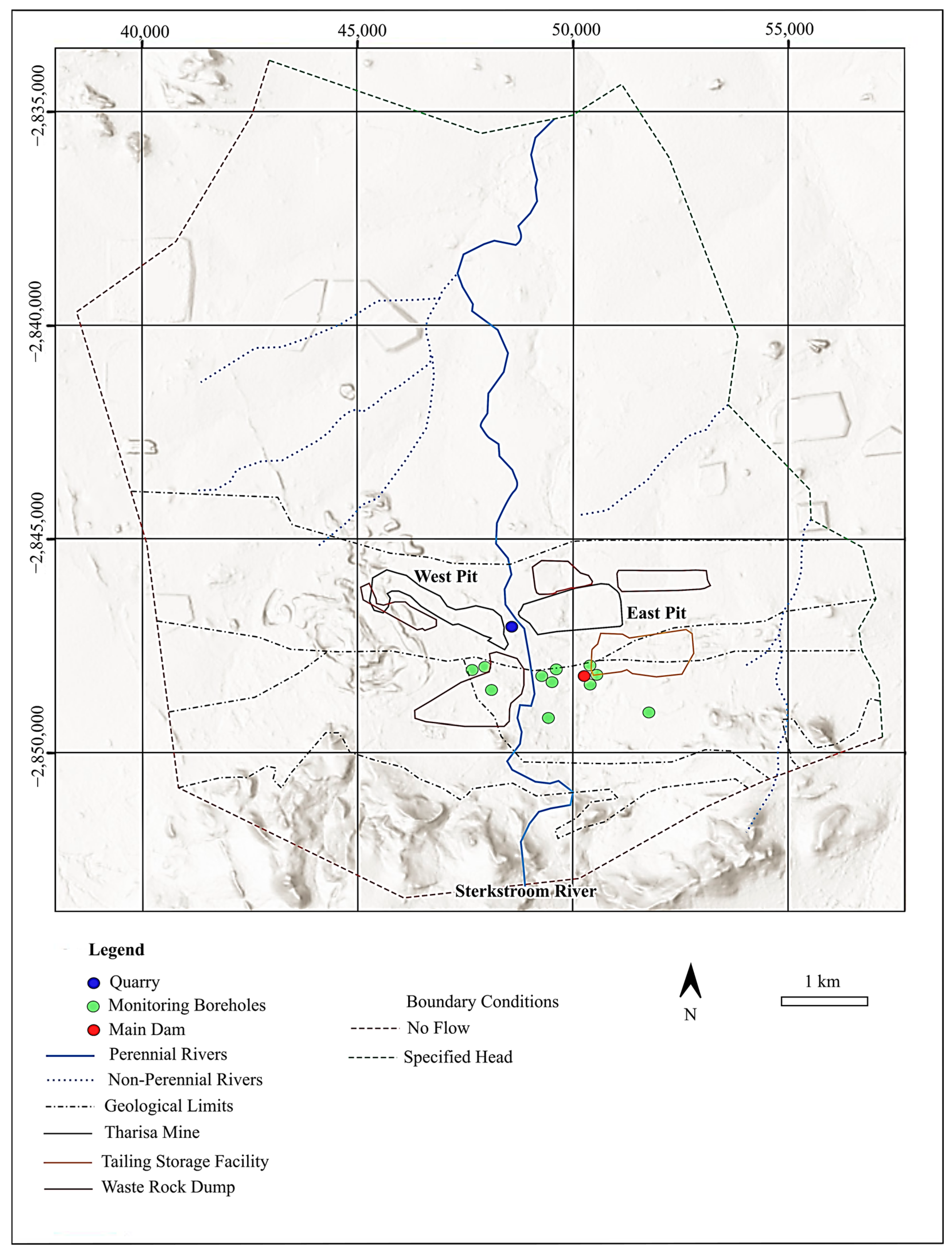
- East Pit: 2698 m3/day (31 L/s);
- West Pit: 1432 m3/day (17 L/s).
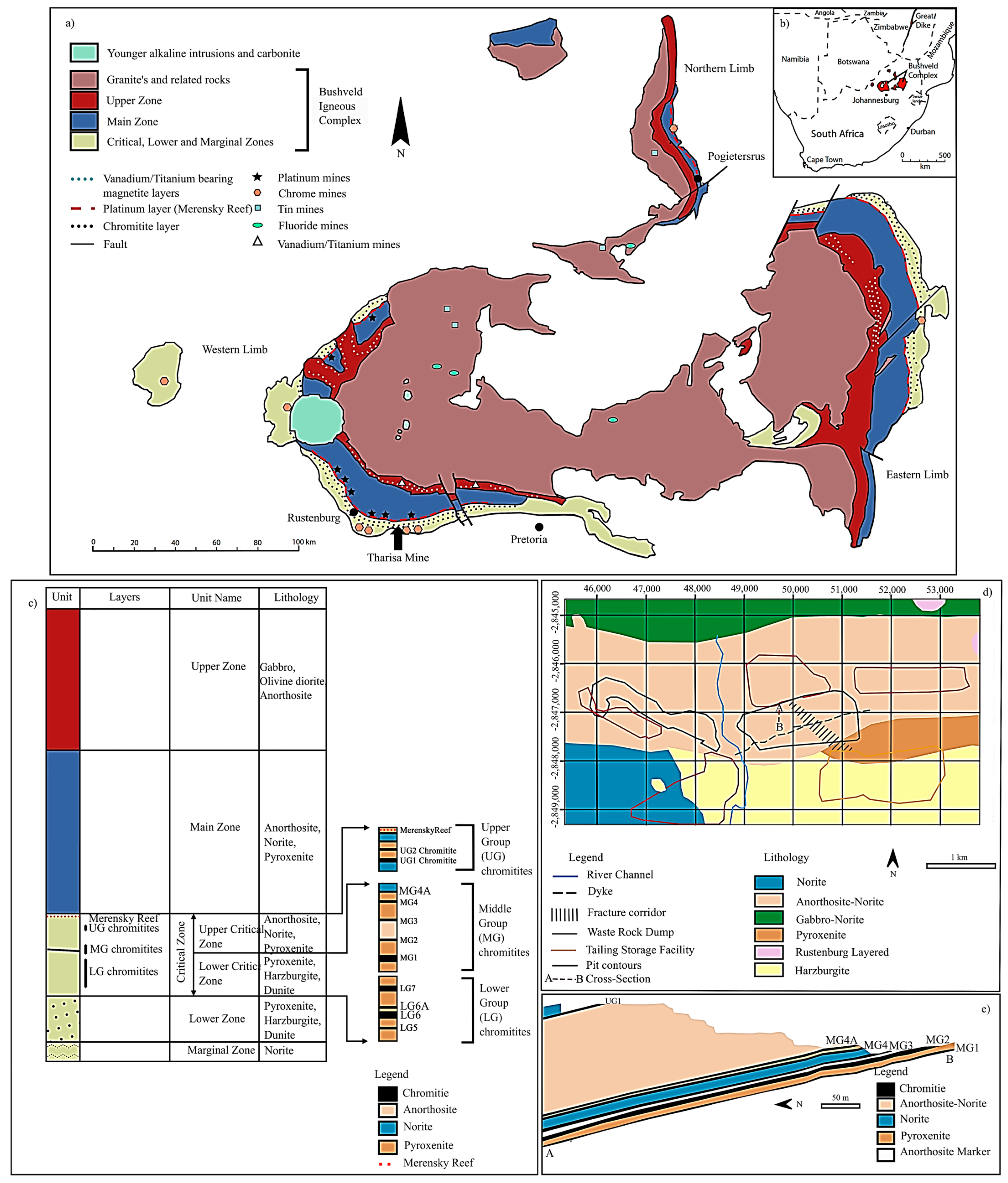
Study Area
- Lower Group (LG) Chromitite Layers;
- Middle Group (MG) Chromitite Layers;
- Unweathered rock matrix with minimal porosity and permeability;
- Rock matrix with discontinuity planes, including faults and joint planes (together referred to as fractures) [45].
- No-Flow Boundary: Along this portion of the model borders, there is no fluid exchange (into or out of the groundwater system). The no-flow boundary was chosen to be along the lines of high elevation that represent watershed boundaries on the southern and western edges of the model domain;
- Specified Head Boundary: Fluid exchange happens both within and outside the model area, ensuring that the hydraulic head boundaries are kept at their initial values:
- External Boundary: along the low-elevation river on the eastern side and partially on the northern side of the model domain limits;
- Internal Boundary: established along the rivers that are a part of the model domain for the groundwater domain [45].
2. Materials and Methods
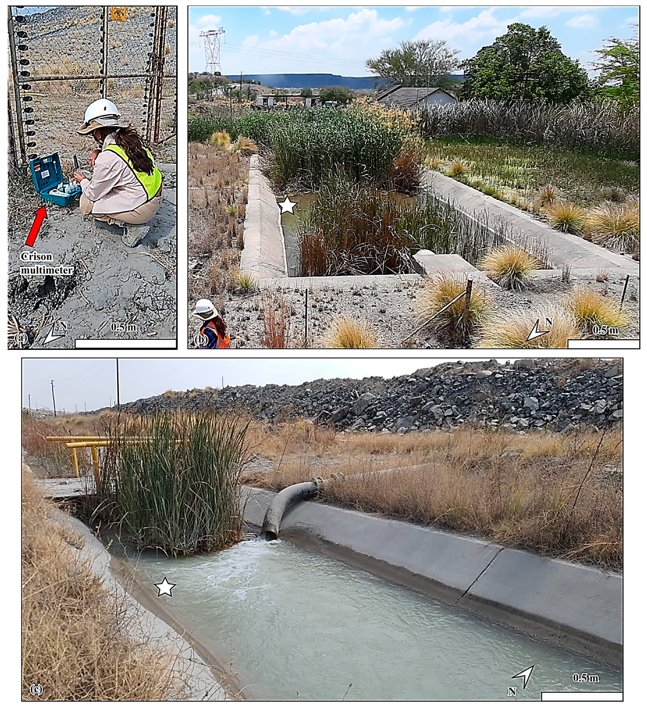
2.1. Water Sampling Methods (Physicochemical Field Parameters): Electrical Conductivity, Total Dissolved Solids, pH, and Temperature
2.2. Environmental Isotopes of Water
2.2.1. δ18O and δ2H
2.2.2. Tritium 3H
2.3. Electrical Resistivity Tomography (ERT)
2.4. Multichannel Analysis of Surface Waves (MASW)
2.5. Seismics
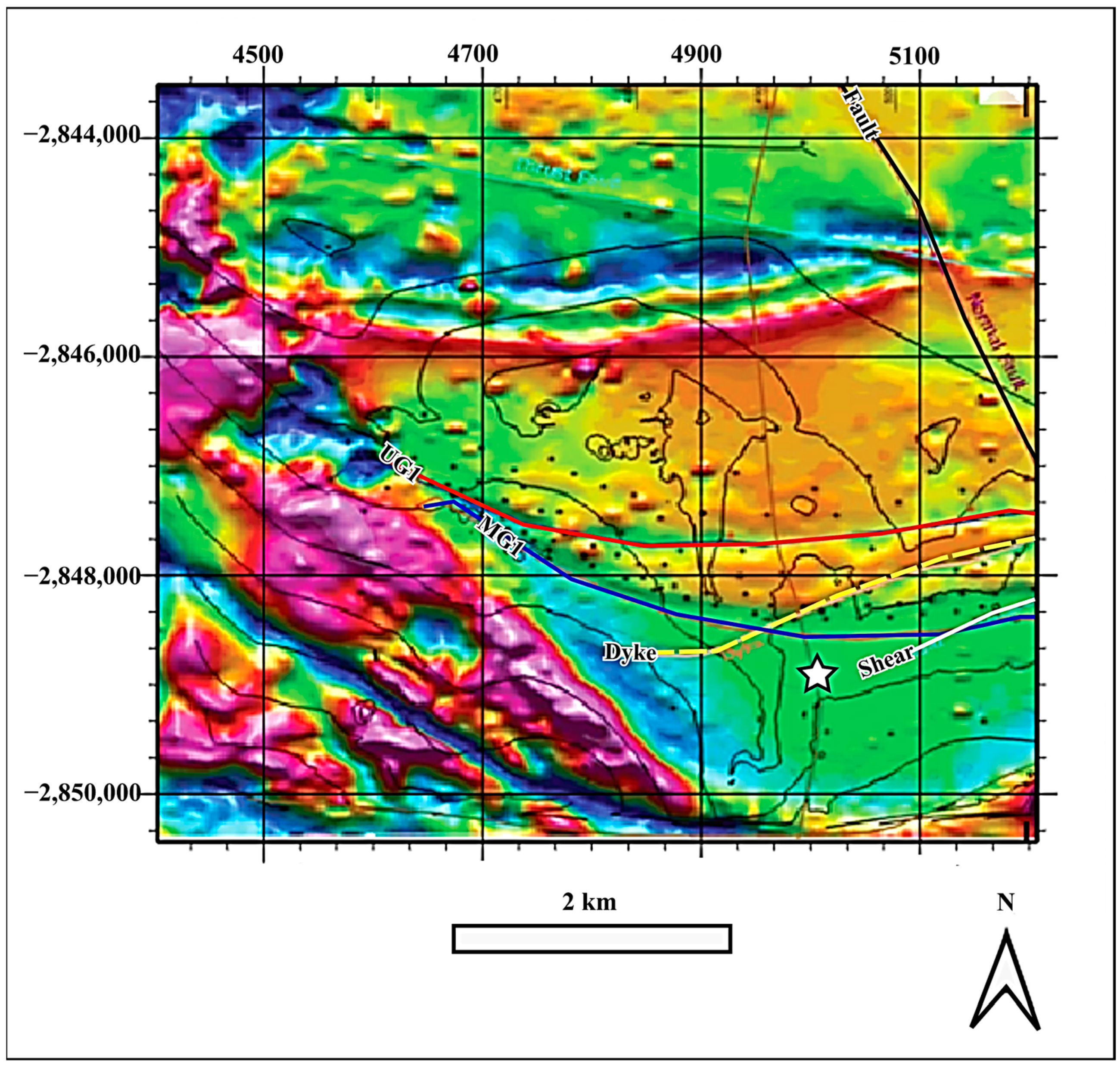
2.6. Magnetics
3. Results
3.1. Hydrogeological Results
3.2. Geophysical Results
4. Discussion
- The majority of groundwater influx volumes may come from different fracture systems or zones;
- By continuously developing the mine, a bigger aquifer volume is reached, promoting rising groundwater inflows into the open pit;
- During mining operations (such as unloading rock masses, blasting operations, and dewatering plans), the aquifer material’s capacity to transfer and retain groundwater is significantly enhanced close to the open pit.
5. Conclusions
Author Contributions
Funding
Data Availability Statement
Acknowledgments
Conflicts of Interest
References
- Lines, G.C. The Ground-Water System and Possible Effects of Underground Coal Mining in the Trail Mountain Area, Central Utah; Department of the Interior, US Geological Survey: Reston, WV, USA, 1985.
- MINEO Consortium. Review of Potential Environmental and Social Impact of Mining; MINEO Consortium: Gela, Italy, 2000. [Google Scholar]
- Environment Australia. Overview of Best Practice Environmental Management in Mining; Environment Australia: Canberra, Australia, 2002. [Google Scholar]
- Mengistu, H.A.; Demlie, M.B.; Abiye, T.A.; Xu, Y.; Kanyerere, T. Conceptual Hydrogeological and Numerical Groundwater Flow Modelling around the Moab Khutsong Deep Gold Mine, South Africa. Groundw. Sustain. Dev. 2019, 9, 100266. [Google Scholar] [CrossRef]
- Szczepiński, J. The Significance of Groundwater Flow Modeling Study for Simulation of Opencast Mine Dewatering, Flooding, and the Environmental Impact. Water 2019, 11, 848. [Google Scholar] [CrossRef] [Green Version]
- Jhariya, D.C.; Khan, R.; Thakur, G.S. Impact of Mining Activity on Water Resource: An Overview Study. In Proceedings of the Recent Practices and Innovations in Mining Industry, Raipur, India, 19–20 February 2016; pp. 271–277. [Google Scholar]
- Yang, Y.; Guo, T.; Jiao, W. Destruction Processes of Mining on Water Environment in the Mining Area Combining Isotopic and Hydrochemical Tracer. Environ. Pollut. 2018, 237, 356–365. [Google Scholar] [CrossRef] [PubMed]
- Ruiz, F.; Gomis, V.; Blasco, P. Application of Factor Analysis to the Hydrogeochemical Study of a Coastal Aquifer. J. Hydrol. 1990, 119, 169–177. [Google Scholar] [CrossRef]
- Subramani, T.; Rajmohan, N.; Elango, L. Groundwater Geochemistry and Identification of Hydrogeochemical Processes in a Hard Rock Region, Southern India. Environ. Monit. Assess. 2010, 162, 123–137. [Google Scholar] [CrossRef] [PubMed]
- Al-Ahmadi, M.E. Hydrochemical Characterization of Groundwater in Wadi Sayyah, Western Saudi Arabia. Appl. Water Sci. 2013, 3, 721–732. [Google Scholar] [CrossRef] [Green Version]
- Chebbah, M.; Allia, Z. Geochemistry and Hydrogeochemical Process of Groundwater in the Souf Valley of Low Septentrional Sahara, Algeria. Afr. J. Environ. Sci. Technol. 2015, 9, 261–273. [Google Scholar] [CrossRef] [Green Version]
- Al-Hmani, A.; Jamaa, N.B.; Kharroubi, A.; Agoubi, B. Assessment of Groundwater in Sana’a Basin Aquifers, Yemen, Using Hydrogeochemical Modeling and Multivariate Statistical Analysis. Arab. J. Geosci. 2022, 15, 684. [Google Scholar] [CrossRef]
- Yihdego, Y.; Webb, J.A.; Leahy, P. Modelling of Lake Level under Climate Change Conditions: Lake Purrumbete in Southeastern Australia. Environ. Earth Sci. 2015, 73, 3855–3872. [Google Scholar] [CrossRef]
- Mogaji, K.A.; Omobude, O.B. Modeling of Geoelectric Parameters for Assessing Groundwater Potentiality in a Multifaceted Geologic Terrain, Ipinsa Southwest, Nigeria—A GIS-Based GODT Approach. NRIAG J. Astron. Geophys. 2017, 6, 434–451. [Google Scholar] [CrossRef] [Green Version]
- Mohamaden, M.I.I.; Hamouda, A.Z.; Mansour, S. Application of Electrical Resistivity Method for Groundwater Exploration at the Moghra Area, Western Desert, Egypt. Egypt. J. Aquat. Res. 2016, 42, 261–268. [Google Scholar] [CrossRef] [Green Version]
- Wattanasen, K.; Elming, S.-Å. Direct and Indirect Methods for Groundwater Investigations: A Case-Study of MRS and VES in the Southern Part of Sweden. J. Appl. Geophys. 2008, 66, 104–117. [Google Scholar] [CrossRef]
- Younis, A.; Soliman, M.; Moussa, S.; Massoud, U.; ElNabi, S.A.; Attia, M. Integrated Geophysical Application to Investigate Groundwater Potentiality of the Shallow Nubian Aquifer at Northern Kharga, Western Desert, Egypt. NRIAG J. Astron. Geophys. 2016, 5, 186–198. [Google Scholar] [CrossRef] [Green Version]
- Song, L.; Zhu, J.; Yan, Q.; Kang, H. Estimation of Groundwater Levels with Vertical Electrical Sounding in the Semiarid Area of South Keerqin Sandy Aquifer, China. J. Appl. Geophys. 2012, 83, 11–18. [Google Scholar] [CrossRef]
- Lopes, D.D.; Silva, S.M.C.P.; Fernandes, F.; Teixeira, R.S.; Celligoi, A.; Dall’Antônia, L.H. Geophysical Technique and Groundwater Monitoring to Detect Leachate Contamination in the Surrounding Area of a Landfill—Londrina (PR—Brazil). J. Environ. Manag. 2012, 113, 481–487. [Google Scholar] [CrossRef] [PubMed]
- Mohamaden, M.I.I.; Ehab, D. Application of Electrical Resistivity for Groundwater Exploration in Wadi Rahaba, Shalateen, Egypt. NRIAG J. Astron. Geophys. 2017, 6, 201–209. [Google Scholar] [CrossRef]
- Ruthsatz, A.D.; Sarmiento Flores, A.; Diaz, D.; Reinoso, P.S.; Herrera, C.; Brasse, H. Joint TEM and MT Aquifer Study in the Atacama Desert, North Chile. J. Appl. Geophys. 2018, 153, 7–16. [Google Scholar] [CrossRef]
- Helaly, A.S. Assessment of Groundwater Potentiality Using Geophysical Techniques in Wadi Allaqi Basin, Eastern Desert, Egypt—Case Study. NRIAG J. Astron. Geophys. 2017, 6, 408–421. [Google Scholar] [CrossRef] [Green Version]
- Binley, A.; Hubbard, S.S.; Huisman, J.A.; Revil, A.; Robinson, D.A.; Singha, K.; Slater, L.D. The Emergence of Hydrogeophysics for Improved Understanding of Subsurface Processes over Multiple Scales. Water Resour. Res. 2015, 51, 3837–3866. [Google Scholar] [CrossRef] [Green Version]
- McLachlan, P.J.; Chambers, J.E.; Uhlemann, S.S.; Binley, A. Geophysical Characterisation of the Groundwater–Surface Water Interface. Adv. Water Resour. 2017, 109, 302–319. [Google Scholar] [CrossRef] [Green Version]
- Singha, K.; Day-Lewis, F.D.; Johnson, T.; Slater, L.D. Advances in Interpretation of Subsurface Processes with Time-Lapse Electrical Imaging: Time-Lapse Electrical Imaging. Hydrol. Process. 2015, 29, 1549–1576. [Google Scholar] [CrossRef]
- Dailey, D.; Sauck, W.; Sultan, M.; Milewski, A.; Ahmed, M.; Laton, W.R.; Elkadiri, R.; Foster, J.; Schmidt, C.; Al Harbi, T. Geophysical, Remote Sensing, GIS, and Isotopic Applications for a Better Understanding of the Structural Controls on Groundwater Flow in the Mojave Desert, California. J. Hydrol. Reg. Stud. 2015, 3, 211–232. [Google Scholar] [CrossRef] [Green Version]
- Wiederhold, H.; Kallesøe, A.J.; Kirsch, R.; Mecking, R.; Pechnig, R.; Skowronek, F. Geophysical Methods Help to Assess Potential Groundwater Extraction Sites. Grund. Z. Fachsekt. Hydrogeol. 2021, 26, 367–378. [Google Scholar] [CrossRef]
- Polom, U.; Bagge, M.; Wadas, S.; Winsemann, J.; Brandes, C.; Binot, F.; Krawczyk, C.M. Surveying Near-Surface Depocentres by Means of Shear Wave Seismics. First Break 2013, 31, 67–79. [Google Scholar] [CrossRef]
- Krawczyk, C.M.; Polom, U.; Trabs, S.; Dahm, T. Sinkholes in the City of Hamburg—New Urban Shear-Wave Reflection Seismic System Enables High-Resolution Imaging of Subrosion Structures. J. Appl. Geophys. 2012, 78, 133–143. [Google Scholar] [CrossRef]
- Pugin, A.J.-M.; Pullan, S.E.; Hunter, J.A.; Oldenborger, G.A. Hydrogeological Prospecting Using P- and S-wave Landstreamer Seismic Reflection Methods. Near Surf. Geophys. 2009, 7, 315–328. [Google Scholar] [CrossRef]
- Burschil, T.; Scheer, W.; Kirsch, R.; Wiederhold, H. Hydrogeological Characterisation of a Glacially Affected Barrier Island—The North Frisian Island of Föhr. Groundw. Hydrol. Instrum. Obs. Tech. 2012, 9, 5085–5119. [Google Scholar] [CrossRef] [Green Version]
- Høyer, A.-S.; Jørgensen, F.; Piotrowski, J.A.; Jakobsen, P.R. Deeply Rooted Glaciotectonism in Western Denmark: Geological Composition, Structural Characteristics and the Origin of Varde Hill-Island: Deeply Rooted Glaciotectonism in Western Denmark. J. Quat. Sci. 2013, 28, 683–696. [Google Scholar] [CrossRef]
- Tamiru, G.; Wiederhold, H. P- and S-Wave Reflection Profiling for near-Surface Investigation of Glacial Sediments. J. Appl. Geophys. 2020, 183, 104216. [Google Scholar] [CrossRef]
- Hoffmann, S.; Beilecke, T.; Polom, U.; Werban, U.; Leven, C.; Engeser, B. Integrierter Einsatz von Scherwellenseismik und Direct-Push-Verfahren zur Erkundung eines urbanen Grundwasserleiters. Grundwasser 2008, 13, 78–90. [Google Scholar] [CrossRef]
- Clarke, B.M. Intrusion Mechanisms of the Southwestern Rustenburg Layered Suite as Deduced from the Spruitfontein Inlier. S. Afr. J. Geol. 2000, 103, 120–127. [Google Scholar] [CrossRef]
- Eales, H.V.; Reynolds, I.M. Cryptic Variations within Chromitites of the Upper Critical Zone, Northwestern Bushveld Complex. Econ. Geol. 1986, 81, 1056–1066. [Google Scholar] [CrossRef]
- Eales, H.V.; Field, M.; De Klerk, W.J.; Scoon, R.N. Regional Trends of Chemical Variation and Thermal Erosion in the Upper Critical Zone, Western Bushveld Complex. Mineral. Mag. 1988, 52, 63–79. [Google Scholar] [CrossRef] [Green Version]
- Eales, H.V.; De Klerk, W.J.; Butcher, A.R. The Cyclic Unit beneath the UG1 Chromitite (UGIFW Unit) at RPM Union Section Platinum Mine—Rosetta Stone of the Bushveld upper Critical Zone? Mineral. Mag. 1990, 54, 23–43. [Google Scholar] [CrossRef] [Green Version]
- Teigler, B.; Eales, H.V.; Scoon, R.N. The Cumulate Succession in the Critical Zone of the Rustenburg Layered Suite at Brits, Western Bushveld Complex. S. Afr. J. Geol. 1992, 95, 17–28. [Google Scholar]
- Cawthorn, R.G. Pressure Fluctuations and the Formation of the PGE-Rich Merensky and Chromitite Reefs, Bushveld Complex. Min. Depos. 2005, 40, 231–235. [Google Scholar] [CrossRef]
- Taylor, C.D.; Schulz, K.J.; Doebrich, J.L.; Orris, G.; Denning, P.; Kirschbaum, M.J. Geology and Nonfuel Mineral Deposits of Africa and the Middle East; Open-File Report; US Geological Survey: Reston, WV, USA, 2009.
- Zientek, M.L.; Causey, J.D.; Parks, H.L.; Miller, R.J. Global Mineral Resource Assessment: Platinum-Group Elements in Southern Africa—Mineral Inventory and an Assessment of Undiscovered Mineral Resources; Scientific Investigations Report; US Geological Survey: Reston, WV, USA, 2014.
- Lourens, P. The Relation between South African Geology and Geohydrology. Ph.D. Thesis, University of the Free State, Bloemfontein, South Africa, 2013. [Google Scholar]
- Titus, R.; Witthüser, K.; Walters, B. Groundwater and Mining in the Bushveld Complex. In Proceedings of the International Mine and Water Conference, Extended Abstracts, Pretoria, South Africa, 19–23 October 2009. [Google Scholar]
- Loseby, B. Tharisa Mine Dewatering Strategy; SLR Consulting (Pty)Ltd.: Johannesburg, South Africa, 2021. [Google Scholar]
- Lomberg, K.; Bornman, H.; Goldschmidt, A.D.; James, J.; Lotheringen, J.; Pheiffer, A.; Stobart, B.; Wiid, G. Tharisa Chrome and PGM Mine; South Africa Competent Persons Report; Coffey Mining(Pty)Ltd.: Johannesburg, South Africa, 2016. [Google Scholar]
- Mazor, E. Chemical and Isotopic Groundwater Hydrology; Marcel Dekker Inc.: New York, NY, USA, 1997; Volume 413. [Google Scholar]
- Dotsika, E.; Lykoudis, S.; Poutoukis, D. Spatial Distribution of the Isotopic Composition of Precipitation and Spring Water in Greece. Glob. Planet. Chang. 2010, 71, 141–149. [Google Scholar] [CrossRef]
- Clark, I.; Fritz, P. Environmental Isotopes in Hydrogeology; CRC Press: Boca Raton, FL, USA, 2013; p. 328. [Google Scholar]
- Abiye, T.A.; Mengistu, H.; Masindi, K.; Demlie, M. Surface Water and Groundwater Interaction in the upper Crocodile River Basin, Johannesburg, South Africa: Environmental Isotope Approach. S. Afr. J. Geol. 2015, 118, 109–118. [Google Scholar] [CrossRef]
- Paz, M.; Alcalá, F.; Medeiros, A.; Martínez-Pagán, P.; Pérez-Cuevas, J.; Ribeiro, L. Integrated MASW and ERT Imaging for Geological Definition of an Unconfined Alluvial Aquifer Sustaining a Coastal Groundwater-Dependent Ecosystem in Southwest Portugal. Appl. Sci. 2020, 10, 5905. [Google Scholar] [CrossRef]
- Rey, J.; Martínez, J.; Mendoza, R.; Sandoval, S.; Tarasov, V.; Kaminsky, A.; Hidalgo, M.C.; Morales, K. Geophysical Characterization of Aquifers in Southeast Spain Using ERT, TDEM, and Vertical Seismic Reflection. Appl. Sci. 2020, 10, 7365. [Google Scholar] [CrossRef]
- Schoor, M.V.; Fourie, C.J.S. Introduction to the Geophysical Methods Applicable to Coal. In A Guide for Applying Geophysics to Coal Mining Problems in South Africa; Struik Nature: South Africa, Workflow;14822. [place unknown]: Coaltech; 2015; pp. 32–99. Available online: http://hdl.handle.net/10204/8280 (accessed on 31 July 2023).
- Martínez-Segura, M.A.; Conesa-García, C.; Pérez-Cutillas, P.; Martínez-Pagán, P.; Vásconez-Maza, M.D. Identifying Changes in Sediment Texture along an Ephemeral Gravel-Bed Stream Using Electrical Resistivity Tomography 2D and 3D. Appl. Sci. 2021, 11, 3030. [Google Scholar] [CrossRef]
- Sendrós, A.; Urruela, A.; Himi, M.; Alonso, C.; Lovera, R.; Tapias, J.C.; Rivero, L.; Garcia-Artigas, R.; Casas, A. Characterization of a Shallow Coastal Aquifer in the Framework of a Subsurface Storage and Soil Aquifer Treatment Project Using Electrical Resistivity Tomography (Port de La Selva, Spain). Appl. Sci. 2021, 11, 2448. [Google Scholar] [CrossRef]
- Alcalá, F.J.; Martínez-Pagán, P.; Paz, M.C.; Navarro, M.; Pérez-Cuevas, J.; Domingo, F. Combining of MASW and GPR Imaging and Hydrogeological Surveys for the Groundwater Resource Evaluation in a Coastal Urban Area in Southern Spain. Appl. Sci. 2021, 11, 3154. [Google Scholar] [CrossRef]
- Malehmir, A.; Durrheim, R.; Bellefleur, G.; Urosevic, M.; Juhlin, C.; White, D.J.; Milkereit, B.; Campbell, G. Seismic Methods in Mineral Exploration and Mine Planning: A General Overview of Past and Present Case Histories and a Look into the Future. Geophysics 2012, 77, WC173–WC190. [Google Scholar] [CrossRef] [Green Version]
- Manzi, M.S.D.; Gibson, M.A.S.; Hein, K.A.A.; King, N.; Durrheim, R.J. Application of 3D Seismic Techniques to Evaluate Ore Resources in the West Wits Line Goldfield and Portions of the West Rand Goldfield, South Africa. Geophysics 2012, 77, WC163–WC171. [Google Scholar] [CrossRef]
- Manzi, M.; Malehmir, A.; Durrheim, R.J. 3D Reflection Seismics for Deep Platinum Exploration in the Bushveld Complex, South Africa. In Proceedings of the 2nd Conference on Geophysics for Mineral Exploration and Mining, Porto, Portugal, 9–12 September 2018; European Association of Geoscientists & Engineers: Porto, Portugal, 2018; pp. 1–5. [Google Scholar] [CrossRef]
- Manzi, M.S.D.; Durrheim, R.J.; Hein, K.A.A.; King, N. 3D Edge Detection Seismic Attributes Used to Map Potential Conduits for Water and Methane in Deep Gold Mines in the Witwatersrand Basin, South Africa. Geophysics 2012, 77, WC133–WC147. [Google Scholar] [CrossRef]
- Pazzi, V.; Di Filippo, M.; Di Nezza, M.; Carlà, T.; Bardi, F.; Marini, F.; Fontanelli, K.; Intrieri, E.; Fanti, R. Integrated Geophysical Survey in a Sinkhole-Prone Area: Microgravity, Electrical Resistivity Tomographies, and Seismic Noise Measurements to Delimit Its Extension. Eng. Geol. 2018, 243, 282–293. [Google Scholar] [CrossRef]
- Robinson, D.A.; Binley, A.; Crook, N.; Day-Lewis, F.D.; Ferré, T.P.A.; Grauch, V.J.S.; Knight, R.; Knoll, M.; Lakshmi, V.; Miller, R.; et al. Advancing Process-Based Watershed Hydrological Research Using near-Surface Geophysics: A Vision for, and Review of, Electrical and Magnetic Geophysical Methods. Hydrol. Process. 2008, 22, 3604–3635. [Google Scholar] [CrossRef]
- Lubczynski, M.; Roy, J. Hydrogeological Interpretation and Potential of the New Magnetic Resonance Sounding (MRS) Method. J. Hydrol. 2003, 283, 19–40. [Google Scholar] [CrossRef]
- World Health Organization. The World Health Report 2007: A Safer Future: Global Public Health Security in the 21st Century; World Health Organization: Geneva, Switzerland, 2007.
- Rusydi, A.F. Correlation between Conductivity and Total Dissolved Solid in Various Type of Water: A Review. IOP Conf. Ser. Earth Environ. Sci. 2018, 118, 012019. [Google Scholar] [CrossRef]
- Porowski, A. Isotopic Evidence of the Origin of Mineralized Waters from the Central Carpathian Synclinorium, SE Poland. Environ. Geol. 2004, 46, 661–669. [Google Scholar] [CrossRef]
- Chilton, P.J.; Foster, S.S.D. Hydrogeological Characterisation and Water-Supply Potential of Basement Aquifers in Tropical Africa. Hydrogeol. J. 1995, 3, 36–49. [Google Scholar] [CrossRef]
- Howard, R.T.K. A Tectono-Geomorphic Model of the Hydrogeology of Deeply Weathered Crystalline Rock: Evidence from Uganda. Hydrogeol. J. 2000, 8, 279–294. [Google Scholar]


| Collection technique | A Crison MM 40 multimeter is used to take an in situ reading. Allow it to stabilize. Samples are to be stored in a cooler box to avoid fractionation. |
| Collection | A sample bottle is used as a means of direct collection of an unfiltered sample. Pre-rinse the sample bottle with sample water before the final collection. |
| Filling technique | The container is tightly capped to the brim to exclude air (air bubbles). |
| Analysis method | The electrode is stored in a KCl solution (electrolyte). Dip the electrode in deionized water and then into the beaker with the water to be measured. Let it stabilize before recording the data. Then, dip the electrode back into the deionized water before storing it in the KCl solution. |
| Description | X | Y | Sample | pH | Temperature (°C) | TDS (mg/L) | EC (µS/cm) | δ2H (‰) | δ18O (‰) | 3H (T.U) |
|---|---|---|---|---|---|---|---|---|---|---|
| River | −48,920.47 | 2,847,915.65 | T3 | 6.8 | 13.3 | 179.4 | 283 | −18 | −3.37 | 1.8 |
| Dissipator Dam 2 | -52,223.74 | 2,846,645.34 | T5 | 7.5 | 16.4 | 886 | 1379 | −5.4 | −1.12 | 2.5 |
| Dissipator Dam 1 | −50,657.04 | 2,846,434.29 | T6 | 7.5 | 15.1 | 589 | 915 | 0.5 | 0.58 | 0.3 |
| Main Dam | −50,470.18 | 2,848,066.6 | T7 | 8.1 | 16.5 | 755 | 1193 | 4.7 | 1.5 | 3.4 |
| Stormwater Dam | −49,453.15 | 2,847,951.97 | T9 | 7.6 | 15.9 | 812 | 1268 | −8.1 | −1.41 | 1.0 |
| West Pit (Dyke) | −48,426.07 | 2,847,589.44 | T1 | 6.2 | 14.5 | 390 | 609 | −16.6 | −3.15 | 0.3 |
| West Pit | −48,261.84 | 2,847,524.26 | T2 | 6.4 | 15.7 | 556 | 873 | −16.8 | −3.2 | 1.6 |
| East Pit | −50,026.53 | 2,847,308.23 | T10 | 7.4 | 19.3 | 949 | 1480 | −13.8 | −2.66 | 2.2 |
| East Pit | −50,023.6 | 2,847,287.17 | T11 | 7.2 | 19.2 | 941 | 1474 | −17.2 | −3.37 | 2.0 |
| East Pit | −50,146.09 | 2,847,268.8 | T12 | 7.4 | 20.8 | 946 | 1475 | −17.1 | −3.41 | 1.6 |
| East Pit | −50,171.71 | 2,847,392.87 | T13 | 8 | 18.3 | 798 | 1248 | −7.6 | −1.75 | 3.2 |
| Est Pit | −49,773.92 | 2,847,504.48 | T14 | 7.7 | 18.7 | 886 | 1383 | −12.8 | −2.42 | 2.9 |
| East Pit | −49,914.75 | 2,847,413.06 | T15 | 7.8 | 19.2 | 848 | 1323 | −11.5 | −2.26 | 1.8 |
| East Pit (Dyke) | −49,184.37 | 2,847,564.54 | T16 | 8.1 | 18 | 784 | 1222 | −14.5 | −2.74 | 2.0 |
| East Pit (Dyke) | −49,240.63 | 2,847,627.68 | T17 | 7.7 | 20.1 | 799 | 1247 | −12.7 | −2.42 | 1.7 |
| East Pit (Dyke) | −49,211.54 | 2,847,624.25 | T18 | 7.9 | 20.6 | 800 | 1247 | −11 | −2.11 | 2.2 |
| East Pit | −50,687.21 | 2,847,441.03 | T19 | 8.2 | 16.7 | 806 | 1260 | −11.4 | −2.4 | 2.3 |
| Far West Pit | −46,531.23 | 2,846,628.66 | T20 | 7.3 | 12.8 | 609 | 950 | −22.8 | −4.63 | 1.4 |
| East Pit | −49,524.01 | 2,847,516.84 | T21 | 7.5 | 13.5 | 872 | 1366 | −10.3 | −1.98 | 2.1 |
| East Pit | −49,424.98 | 2,847,702.59 | T22 | 7.36 | 22.3 | 947 | 1295 | −9.2 | −2.15 | 2.1 |
| Quarry | −48,941.16 | 2,847,746.22 | T8 | 7.7 | 16.7 | 837 | 1303 | −11.2 | −1.92 | 1.0 |
| Samancor Borehole | −52,223.74 | 2,846,645.34 | T4 | 6.7 | 21.6 | 1450 | 2230 | −18.8 | −3.79 | 1.1 |
| Monitoring Borehole (TM GW FW BH 24) | −47,662.66 | 2,846,946.1 | T24 | 6.84 | 23.5 | 537 | 839 | −24 | −3.5 | 2.0 |
| Monitoring Borehole (TM GW FW BH 25) | −48,480.54 | 2,847,484.17 | T25 | 7.5 | 20.1 | 669 | 1046 | −17.4 | −3.77 | 2.1 |
| Monitoring Borehole (TM GW Dissipater 1) | −50,603.6 | 2,848,077.08 | T26 | 6.67 | 21.3 | 684 | 1067 | −5.9 | −0.17 | 1.1 |
| Monitoring Borehole (TM GW Dissipater 2) | −50,591.71 | 2,848,037.15 | T27 | 6.98 | 21.9 | 693 | 1082 | −6.6 | −0.83 | 1.5 |
| Monitoring Borehole (TM GW RPM) | −50,431.98 | 2,848,085.29 | T28 | 7.29 | 20.9 | 714 | 1115 | −11.5 | −1.83 | 1.5 |
| Monitoring Borehole (TM GW COMM 02) | −51,747.65 | 2,849,061.98 | T29 | 7.14 | 21.3 | 332 | 519 | −0.8 | 0.61 | 1.9 |
| Monitoring Borehole (TM GW COMM 01) | −49,472.5 | 2,849,217.25 | T30 | 7.33 | 21.9 | 367 | 575 | −15.9 | −2.9 | 1.5 |
| Monitoring Borehole (TM GW TSF 01) | −50,127.44 | 2,849,013.64 | T31 | 7.32 | 21.3 | 344 | 536 | −12.5 | −2.04 | 1.3 |
| Monitoring Borehole (TM GW COMM 06) | −48,075.45 | 2,848,504.16 | T32 | 7.15 | 22.6 | 296 | 464 | −11.8 | −1.93 | 1.9 |
Disclaimer/Publisher’s Note: The statements, opinions and data contained in all publications are solely those of the individual author(s) and contributor(s) and not of MDPI and/or the editor(s). MDPI and/or the editor(s) disclaim responsibility for any injury to people or property resulting from any ideas, methods, instructions or products referred to in the content. |
© 2023 by the authors. Licensee MDPI, Basel, Switzerland. This article is an open access article distributed under the terms and conditions of the Creative Commons Attribution (CC BY) license (https://creativecommons.org/licenses/by/4.0/).
Share and Cite
Dildar, J.; Manzi, M.S.D.; Abiye, T.; Gomo, S.; Rapetsoa, M.K.; Drennan, G. Groundwater Circulation in the Shallow Crystalline Aquifer of Tharisa Mine, South Africa: Evidence from Environmental Isotopes and Near-Surface Geophysics. Water 2023, 15, 2876. https://doi.org/10.3390/w15162876
Dildar J, Manzi MSD, Abiye T, Gomo S, Rapetsoa MK, Drennan G. Groundwater Circulation in the Shallow Crystalline Aquifer of Tharisa Mine, South Africa: Evidence from Environmental Isotopes and Near-Surface Geophysics. Water. 2023; 15(16):2876. https://doi.org/10.3390/w15162876
Chicago/Turabian StyleDildar, Jureya, Musa Siphiwe Doctor Manzi, Tamiru Abiye, Sikelela Gomo, Moyagabo Kenneth Rapetsoa, and Gillian Drennan. 2023. "Groundwater Circulation in the Shallow Crystalline Aquifer of Tharisa Mine, South Africa: Evidence from Environmental Isotopes and Near-Surface Geophysics" Water 15, no. 16: 2876. https://doi.org/10.3390/w15162876
APA StyleDildar, J., Manzi, M. S. D., Abiye, T., Gomo, S., Rapetsoa, M. K., & Drennan, G. (2023). Groundwater Circulation in the Shallow Crystalline Aquifer of Tharisa Mine, South Africa: Evidence from Environmental Isotopes and Near-Surface Geophysics. Water, 15(16), 2876. https://doi.org/10.3390/w15162876