Article

Integrated Hydrogeological Modelling for Sustainable Management of the Brindisi Plain Aquifer (Southern Italy)

by
Nicola Pastore
1,*,
Claudia Cherubini
2,* and
Concetta Immacolata Giasi
1
1
Department of Civil, Environmental and Structural Engineering and Chemistry (DICATECh), Polytechnic of Bari, Via E. Orabona 4, 70125 Bari, Italy
2
Department of Environmental and Prevention Sciences, University of Ferrara, Via Saragat 1, 44122 Ferrara, Italy
*
Authors to whom correspondence should be addressed.
Water 2023, 15(16), 2943; https://doi.org/10.3390/w15162943
Submission received: 21 July 2023 / Revised: 31 July 2023 / Accepted: 4 August 2023 / Published: 15 August 2023
(This article belongs to the Special Issue Groundwater: The Processes and Global Significance of Aquifers)

Abstract

:
Nowadays, changes in precipitation patterns together with the increasing water demand impose a sustainable management where the budget between water availability and demand is positively closed. A parsimonious hydrogeological modelling approach coupled with a soil water balance is developed and applied in order to quantify the hydrological and hydrogeological dynamics in a semi-arid region of the Mediterranean basin. In particular, the present work focuses on the hydrogeological dynamics of the catchment areas of Siedi, Foggia di Rau, Pigonati, and the Palmarini channels located in the Brindisi Plain, Southern Italy. In the last decades, in the Brindisi Plain the anthropization processes as well as the industrial and agricultural development have generated an intensive exploitation of both shallow and deep groundwater resources as well as their qualitative deterioration. A dry hydrologic year (2019–2020) caused a recharge deficit, resulting in a lowering of the groundwater level of the shallow aquifer compared to the expected seasonal value. The results evidence a sensitive natural system, where the variability of the rainfall regime combined with water withdrawal leads to a system that is very vulnerable to climate change impacts, such as the presence of erratic rainfall patterns affecting aquifer recharge. This study represents the first approach to couple a soil moisture balance model and groundwater flow model to assess the impact of changes in rainfall patterns on groundwater recharge for the Brindisi Plain aquifer. The developed integrated hydrogeological model can be applied to other sites with similar hydrogeological features and represents an important tool in order to evaluate the effectiveness of cost-effective sustainable actions for the management of the groundwater resources with respect to land-use practices and socio-economic aspects.

1. Introduction

Nowadays, changes in precipitation patterns are impacting people and ecosystems by altering the availability of water throughout the year. Studies conducted at different scales recognize that the impact of anthropogenic stresses and altered rainfall patterns on surface water and groundwater varies according to geographic locations [1].
In southern Europe, the Mediterranean region has been identified as a “climate change hot-spot” [2] in that it is projected to undergo a large decrease in mean precipitation and an increase in precipitation variability during the dry (warm) season.
The climate of Mediterranean semi-arid regions is characterized by irregularly distributed rainfall in time and space and sometimes very high and intense anthropogenic stresses. In these climate scenarios, worsened by an increase of extreme rainfall events coupled with the decrease of annual rainfall [3], aquifer recharge may also be affected. Groundwater is the most important natural resource [4] and it is a critical factor in the water management of a catchment area for various requirements (agricultural, industrial, and domestic) in both rural and urban areas. Sustainable management of the groundwater resources needs a detailed representation of groundwater flow dynamics in terms of recharge and discharge as well as storage changes [5]. It is therefore necessary to understand groundwater recharge characteristics, its space and time variations, and factors controlling the interaction between surface water and groundwater [6,7].
The integrated hydrological modelling represents a key tool for decision support to improve water resources’ management [8,9,10,11,12]. On the other hand, sustainable groundwater management requires a numerical model which is able to represent the whole flow dynamics with small computational costs [13]. For a catchment area, the Soil Moisture Balance (SMB) model at daily scale is a valuable approach to determine the components of the hydrologic cycle [14]. Then, net infiltration is estimated, representing the quantity of water moving downwards from the soil zone as potential aquifer recharge [15,16,17].
Among the Mediterranean areas, a very vulnerable region is Apulia (south-eastern Italy) which, in absence of surface water, relies on groundwater to meet all water requirements. A particularly sensitive area in Apulia is characterized by the Brindisi Plain: a large portion of sub-flat territory between the offshoots of the limestone bank of the Murge to the north-west and the weak undulations of northern Salento to the south.
In this area, characterized by a semi-arid climate, the shallow aquifer is exploited mainly for domestic purposes and secondarily for agriculture by means of dug wells. Due to natural gas pipe line installation, shallow groundwater level time series are collected in the Terra Rossa district located in Tuturano within the Brindisi Plain. Actually, approximately 400 habitants live in the Terra Rossa district with precarious sanitary conditions due to incompleteness of primary urbanization works such as water supply, sewers, and public lighting. The shallow groundwater represents the only water resource exploited with dug wells. During summer 2020, the groundwater level of the shallow aquifer decreased considerably with respect to its normal condition, and the dug wells went dry.
This area has been the object of previous hydrogeological investigations in the past but most of them regarded qualitative studies [18,19,20] and a data-driven approach to infer groundwater system dynamics [21,22].
The previously carried out studies cannot be employed to improve local groundwater governance, i.e., for groundwater management planning, to design interventions, or to simulate scenarios on the aquifer. Physically based numerical models are essential for simulating hydrogeological processes and guiding informed policy-making for sustainable groundwater management.
Until now, no study has dealt with numerical groundwater quantity assessment by means of a physically based numerical model in the Brindisi Plain. The present study presents a physically based approach to investigate the hydrological and hydrogeological dynamics of the shallow aquifer of the Brindisi Plain, by determining the relation between precipitation, irrigation, evapotranspiration, infiltration, aquifer exploitation, as well as aquifer recharge and discharge. In particular, the present work focuses on the catchment area of Siedi, Foggia di Rau, Pigonati, and the Palmarini channels. The aim is to investigate the relationship between changes in precipitation patterns and aquifer response to explore the complexity of the hydrogeological processes which caused groundwater depletion, with the perspective to evaluate climate resilience actions for the management of groundwater resources.
A parsimonious methodology is used, based on a daily SMB model [15] linked to a groundwater flow numerical model [23] to investigate the hydrogeological dynamics at daily scale.
For the investigated period (2017–2021), the annual precipitation decreased leading to a drastic reduction of the net infiltration from topsoil to the aquifer, representing the main cause of aquifer depletion. A further consequence of the decrease of groundwater level was the reduction of the discharge rate along the hydrographic network and then through the wetland areas which represent an important natural reserve. On the other hand, due to the changes of the precipitation patterns, the decrease in annual precipitation does not correspond to a decrease in runoff which remains almost constant over time.
The specific goals of this paper are:
  • Improving the understanding of the hydrogeological behavior of the Brindisi Plain shallow aquifer.
  • Evaluating the main cause of aquifer depletion.
  • Testing and validating the developed hydrogeological tool for aquifer management.
Though it is applied to a specified area, the proposed analysis can be extended to other sites with similar hydrogeological features.

2. Materials and Methods

2.1. Study Area

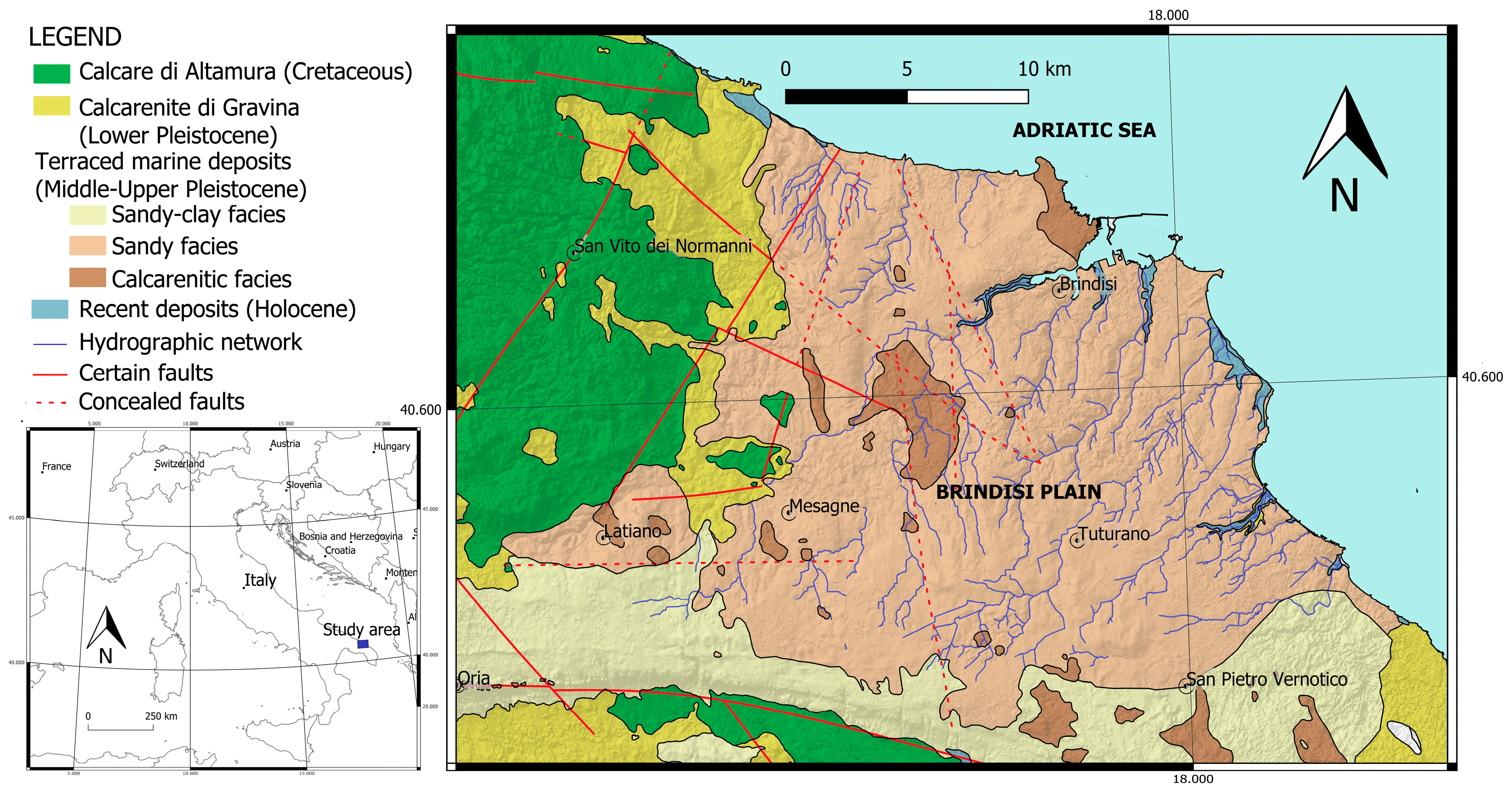
The Brindisi Plain has an extension of 407.78 km2 and a mean elevation of 21.89 m above mean sea level (amsl), facing the Adriatic Sea in the Apulia region (southeastern Italy) (Figure 1). The climate is semi-arid, with an annual long-term mean precipitation of 571.74 mm/year (2011–2021). Natural vegetation and agricultural land cover approximately 3.38% and 82.44%, respectively.

2.2. Geological and Hydrogeological Setting

From the morphological point of view, the Brindisi Plain was conditioned by the glacio-eustatic oscillations of the sea level that occurred in the late Pleistocene and Holocene periods, giving rise to a series of marine transgression/regression cycles that had modelled the landscape. These erosion phenomena are superimposed on the morphogenetic mechanisms of the continental environment, giving rise to a hydrographic network consisting of shallow and poorly hierarchical channels. The erosive incisions (furrows and canals) originate largely in the hilly area, and they develop in the NE–SW direction.
The geology of the Brindisi Plain depicts the structural geological asset of the Apulian foreland [24]. The calcareous-dolomitic succession of the Calcare di Altamura formation (Cretaceous) represents the oldest geological formation. The succession presents a sub-horizontal asset characterized by an irregular alternation of calcareous, calcareous-dolomitic lithotypes variously fissured and karstified. The geologic structure of the succession is characterized by a tectonic disjunctive style regulated by a double system of faults mainly oriented in a NW–SE and E–W direction and secondarily directed NE–SW [25]. The carbonate bedrock degrades with a Horst and Graben structure, towards the Adriatic coast, where it is detectable at a depth of approximately 40 m amsl.
The Calcarenite di Gravina formation (Lower Pleistocene) is found locally in transgression above the carbonate bedrock [26]. The formation is constituted by white-yellowish biocalcarenites, with medium or medium-coarse grain size, with a medium–low cementation degree, usually tender and porous, arranged in thick layers and banks.
In continuity of sedimentation on the Calcareniti di Gravina formation, the Sub-Apennine Clays formation (Lower Pleistocene) is detectable. These soils consist of sandy-clayey silts and marly-silty clays of a gray-blue color. The clay content generally tends to increase in the lower part of the formation, while towards the top the sandy-silty component is prevalent. The top of the clays presents a generalized immersion to the NE, passing from an altitude over 70 m amsl in the Mesagne area to −10 m amsl in the Brindisi area. The thickness of the Sub-Apennine Clays can vary from 5 to 50 m. Generally, the thickness of the clayey formation increases towards the southern part of the Brindisi Plain and near the coast.
In transgression on the Sub-Apennine Clays, the terraced marine deposits (Middle-Upper Pleistocene) outcrop extensively in the study area. This unit is constituted by two main lithofacies with heterotopic contact. The first of the facies is the one that outcrops diffusively in the Brindisi area. It consists of clayey sands and gray-bluish clays with bioclastic arenaceous and calcarenitic interbedding. The second of the facies consists of poorly cemented calcareous sands with limestone interbedding. The terraced marine deposits present a sub-horizontal bedding with a thickness of 20–25 m at most [18]. The top of the deposits is constituted by an abrasion surface constituted from eight different (terraced) locations often covered by recent continental deposits.
The recent deposits (Holocene) of alluvial, colluvial, and marshy origin are found mainly at the bottom of the main canals as well as in the morphological depressions that host coastal ponds or lagoons.
The stratigraphic and structural features of the area allow the existence of two distinct aquifers located within the permeable formations.
The deep aquifer lies within the Mesozoic basement (Calcare di Altamura). The water supply of the deep aquifer is mainly guaranteed by the infiltrating rainwater, taking place essentially in those areas where the limestone rocks outcrop or where these ones are covered by permeable sediments of small thickness. In the study area, except for the area near the coast where clayey deposits force water to circulate under confined conditions, water circulates under phreatic conditions [27] with a groundwater level at most 2.5–3.0 m amsl. The hydraulic gradient, oriented toward to the coast, presents a value of 0.05%. Even at some distance to the coast [28] the freshwater floats on seawater of continental intrusion, flowing towards the Adriatic Sea through the coastal springs.
The shallow aquifer circulates within the sandy-calcarenitic aquifer of the terraced marine deposits, supported at the base by the almost impermeable clayey levels. The shallow aquifer lies largely on the Brindisi Plain and has a variable saturated thickness from 10 m up to 30 m in the Brindisi district [20]. It is usually found a few meters from the ground level with the water circulating everywhere in phreatic conditions.
The shallow aquifer is fed by infiltrating rainfall. The groundwater level is characterized by significant seasonal excursions characterized by a recharge phase during the rainy season and a recession phase during the dry season. The piezometric surface is influenced by aquifer permeability, surface morphology, and the shape of the top of the clayey unit. Groundwater circulates from the hinterland towards the Adriatic coast. The hydrographic network exerts a drainage action limiting the direct flow towards the Adriatic Sea. Moreover, the hydrographic network is characterized by an intermittent regime where significant flows occur only during intense and prolonged rainfall.

2.3. Field Site Description and Characterization

The aim of this work is to investigate the hydrogeological dynamics of the shallow aquifer in correspondence with the Terra Rossa district in order to evaluate the response of the natural system to the variability of the climatic condition and the anthropic stresses. For this purpose, catchment areas of the Siedi, Foggia di Rau, Pigonati, and Palmarini channels were considered (Figure 2). The investigated area has an extension of 175.16 km2 with an elevation range from −1.48–79.71 m amsl.
Shallow piezometers (P1, P2, P3, P4 and P5) were installed within a cored borehole with a diameter of 0.18 m. Piezometers present a depth of 8 m. Filter is located between 4 and 8 m deep. Water levels of the shallow aquifer were recorded monthly from August 2018–September 2021. Daily rainfall and temperature data were available from three meteo-climatic stations located at Brindisi, Mesagne, and Cellino S. Marco. Other climatic data, needed to determine the reference potential evapotranspiration by means of the Penmann-monteith equation such as solar radiation, relative humidity, and wind, were derived from Modern-Era Retrospective Analysis for the Research and Applications project (MERRA—2) [29]. Moreover, three field test sites have been setup during the shallow aquifer characterization. In each field site, geognostic surveys, slug tests, and single-ring infiltrometer tests were carried out. Furthermore, the topsoil was classified from physical and textural points of view.

2.3.1. Single-Ring Infiltrometer Tests

Single-ring infiltrometer tests with variable head were performed. The tests were carried out at a predetermined height of −1.0 m from the ground level in order to exclude the topsoil cover, making a horizontal work surface that was not disturbed much by the excavation operations. The infiltrometer presented an internal diameter of 0.60 m and a height of 0.40 m. The single-ring infiltrometer was driven vertically by beating for 0.05–0.10 m taking care to minimize the disturbance of the horizontal work surface. In the presence of consolidated materials such as calcarenite levels the outer edge of the single ring was sealed with waterproof cement mix. The tests were carried out starting from natural soil moisture conditions with an initial hydraulic level with respect to the horizontal work surface Z0 = 0.3 m and measuring the value reached by the hydraulic level Z(t) with geometric progression in time. A method proposed by Nimmo et al. (2009) [30] was used for the interpretation of the single-ring infiltrometer tests.
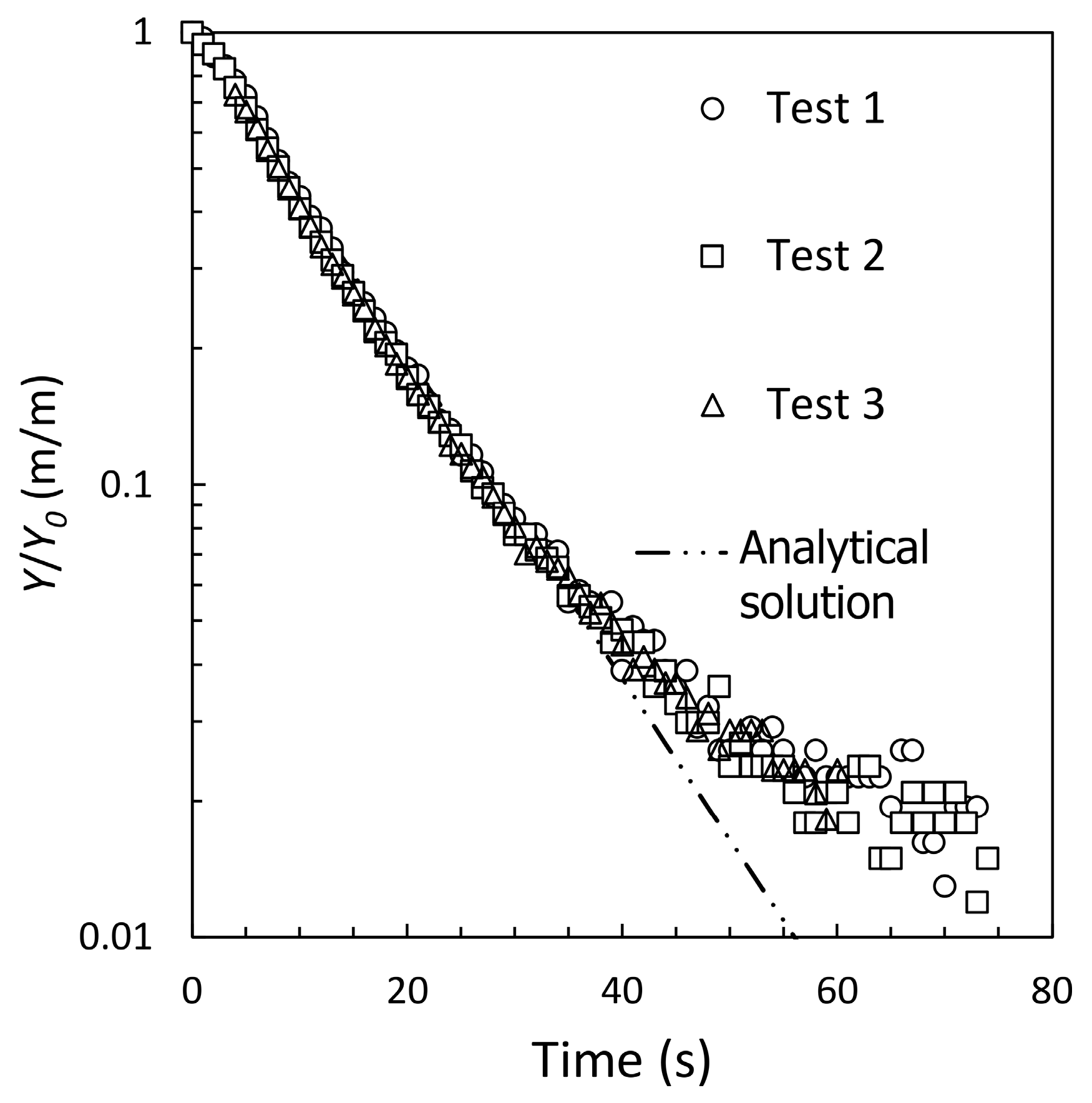
2.3.2. Slug Tests

In order to estimate the hydraulic conductivity of the shallow aquifer, several slug tests were carried out. The tests were performed in partially penetrated piezometers with an inner diameter of 0.10 m by sharply increasing the groundwater level (by adding a volume of water of 10 L) and monitoring the consequent decline of the groundwater level created by the flow from the piezometer towards the aquifer by means of a pressure transducer. Methods proposed by Bouwer (1989) [31] are used for the interpretation of the slug tests.

2.4. Groundwater Exploitation and Land Managment

In the last decades, in the Brindisi Plain catchment the anthropization processes as well as industrial and agricultural development generated an intensive exploitation of both shallow and deep groundwater resources as well as their qualitative deterioration.
A dense irrigation network is present that exploits both shallow and deep aquifers. The shallow aquifer is exploited by dug wells with variable depth between 3 and 20 m only for domestic and agricultural purposes. The deep aquifer is exploited through drilled wells for industrial and agriculture purposes. The shallow aquifer, due to its modest water potential, in the last decades has been exploited mainly for domestic use and secondarily for agricultural purposes, leaving to the deep aquifer the task of covering a larger part of the agricultural and industrial water demand. According to local agricultural practices, the aquifer exploitation is active from May to October with a peak in July.
Agricultural land use covers 85.8% of the investigated area. Four classes of agronomic uses of the topsoil can be detected (Figure 3). The arable land presents both intensive and extensive agriculture. In intensive agriculture, the land is cultivated with vegetables such as tomatoes, cauliflower, watermelons, and artichokes. In extensive agriculture, the arable land can be cultivated with cereals, otherwise it remains uncultivated with the development of herbaceous vegetation. In the whole Brindisi catchment area, the irrigated arable land presents a high irrigation demand of 1796 m3/ha due to the presence of vegetables such as tomatoes and artichokes. Olive groves, vineyards, and orchards present an irrigation demand of 765 m3/ha, 1682 m3/ha, and 2773 m3/ha, respectively.

2.5. Conceptual and Mathematical Models

The observations described in the previous section allowed the establishment of the conceptual model of the shallow aquifer hydrodynamics. The estimation of the quantity of water moving downward from the topsoil as potential recharge is crucial to predict the shallow groundwater dynamics. The shallow aquifer is fed directly by the net infiltration through the vadose zone reaching the groundwater level that is subject to significant seasonal oscillations in response to the direct seasonal recharge events. The shallow groundwater discharges mainly on the hydrographic network along its deeper incisions located near the coastal area. The interaction between the Adriatic Sea and the shallow aquifer occurs only where the bottom of the latter is below the mean sea level. The hydrographic network is characterized by an intermittent regime. It is affected by significant flows for a short time, under intense and prolonged rainfall only. Then, at the temporal scale of the investigation, the recharge component from the hydrographic networks towards the shallow aquifer can be neglected.
A modification of the soil water balance model (SWBM) at daily scale presented by [15] was linked to MODFLOW—2005 [23], in order to analyze the hydrological cycle, groundwater, unsaturated zone, and surface water dynamics. For convenience, a brief introduction of the used computational models is described in the next sections.

2.5.1. Soil Water Balance Model

The soil water balance on a daily scale referred to the topsoil is determined as follows [32]:
W t = W t 1 + P t + I r , t D t E T a , t I n , t ,
where t and t − 1 stand for current day and previous day, respectively, W (mm) is the soil water content, P (mm) is the daily rainfall, Ir (mm) is the contribution of irrigation, D (mm) is the runoff, ETa (mm) is the actual evapotranspiration, and In (mm) is the net infiltration.
The curve number method is used to determine the runoff rate D expressed as [33]:
D = P 0.2 S 2 P + 0.8 S     P > 0.2 S ,  
where S is the potential maximum retention determined as:
S = 25.4 1000 C N 10 ,  
The specific volume of soil saturation is defined by the curve number CN as a function of land use and its infiltration capacity. CN varies in the range 0–100 and it can be associated with three antecedent moisture classes denoted by I, II, and III, and is determined using the 5-day antecedent rainfall depth. Then, the value for class II (CNII) can be estimated on the basis of soil type and land use. For dry (class I) and wet (Class III) conditions, CNI and CNIII, respectively, can be estimated as:
C N I = 4.2 C N I I 10 0.058 C N I I ,  
C N I I I = 23 C N I I 10 + 0.13 C N I I ,  
The crop potential evapotranspiration ETc (mm) can be determined as the product between the reference potential evapotranspiration ET0 (mm) estimated by the Penman–Monteith equation and the crop coefficient Kc which depends on the type of crop and the growth stage of the crop [34].
The actual evapotranspiration ETa is less than its potential value (ETc) when the topsoil is under stress. Then ETa is equal to the product between ETc and Ks. The stress factor Ks is the function of the total and readily available water which depends on the depth of root and soil properties.
For a given topsoil with crop, the total available water TAW (mm) can be defined as:
T A W = θ F C θ W P Z w ,
where θFC (m3/m3) and θWP (m3/m3) are the soil moisture content at Field Capacity (FC) and Wilting Point (WP), respectively, and Zw (m) is the rooting depth of the crop. The Readily Available Water (RAW) can be defined as:
R A W = p · T A W ,
where the factor p varies between 0.2 and 0.7.
The soil moisture deficit SMD (mm) represents the amount of water needed to bring the soil moisture content back to field capacity. If SMD is less than RAW, Ks will be equal to 1. Otherwise, if SMD is greater than TAW, Ks will be equal to 0. In the other cases:
K s = T A W S M D T A W R A W ,  
When SMD is great and there is a significant rainfall, the moisture is retained on the ground surface. This happens especially when the soil has a consistent clay content. The moisture retained on the ground surface NS (mm) can be determined as:
N S t = f s P e , t E T c , t   i f   P e , t > E T c , t 0   o t h e r w i s e ,
where fs is an empirical factor, Pe is the rainfall rate that actually infiltrated the soil and is derived as:
P e , t = P t + I r , t D t + N S t 1 .
The daily SMD balance can be written as:
S M D t = S M D t 1 P e , t + N S t + E T a , t .
The surplus of water with respect to S M D = 0 is the potential recharge, In, that percolated through the vadose zone reaching the water table. Then, when S M D t < 0 , I n , t = S M D t and S M D t = 0 .
For each i-th meteo-climatic station and for each j-th land use, the components of the daily soil moisture balance can be determined. Then, their variation in space and time is determined by means of inverse distance weighting algorithm.

2.5.2. Groundwater Flow Model

MODFLOW—2005, a finite difference groundwater flow model, is used to simulate the groundwater flow dynamics. A finite difference mesh was used to discretize the investigated area. In order to have a reasonable computational cost, it is discretized by a regularly spaced grid of 197 columns and 205 rows with cell size of 104 m2. Vertically, the model consists of a single layer to represent the shallow aquifer which flows in the terraced marine deposits. The layer top elevation is extracted from the DEM with a resolution of 8 m. The layer bottom elevation is derived by the interpretation of the geological surveys in the whole Brindisi Plain catchment area.
The spatial and temporal evolution of the potential recharge determined by means of the SMB model is passed to the UZF package [35] as infiltration. Then, the UZF is used to simulate the infiltration process along the vadose zone.
According to the conceptual model, discharge dynamics along the hydrographic network and wetland area are simulated as drain boundary conditions through the DRN package [23]. The specific discharge flow along the generic i-th reach qi (m3 d−1) is given by:
q i = C i H Z i , t o p   w i t h   H > Z i , t o p .
where Ci (m/d) represents the conductance of the generic reach, Zi,top (m amsl) is the reach elevation, and H (m amsl) is the groundwater level. The conductance term Ci is the function of the reach geometry and its hydraulic properties and is given by:
C i = K i w i t i ,
where Ki (m/d), ti (m), and wi (m) are the hydraulic conductivity, the thickness of the alluvial deposits, and the channel width of the generic i-th reach, respectively.
In correspondence with the coast where the layer bottom is below the mean sea level a constant head boundary condition is applied through the CHD package [23].
According to local knowledge, a random spatial distribution of dug wells within agricultural land with a density of 0.1 Well/ha was used. The dug wells were active from May to October with a peak in July. Then, constant flow boundary condition is used in correspondence with each dug well through the WELL package [23].

3. Results

3.1. Shallow Aquifer Characterisation

3.1.1. Stratigraphy and Lithology

The geognostic surveys carried out in the study area highlight the lithological succession showed in Figure 4. At field test sites, terraced marine deposits outcrop almost everywhere, with the exception of small strips of alluvial deposits that are detectable in very limited territorial areas in correspondence with the channels.
The topsoil presents a sandy clay loam texture with an average sand content of 69.1% and an average clay content of 24.8%. Table 1 summarizes the general and granulometric characteristics determined from sample characterization of the lithological units that constituted the shallow aquifer.

3.1.2. Slug Tests

The interpretation of the slug tests gave an estimation of the saturated hydraulic conductivity of the shallow aquifer at field test sites F1, F2, and F3 (Figure 2). Figure 5 shows the interpretation of the slug tests by means of the Bouwer and Rice equation [31] conducted at the F2 location in a partially penetrated piezometer with a radius of the well casing of 0.05 m, the radius of the gravel enveloped of 0.09 m, the length of screened open section of 3.89 m, and height of saturated thickness of 4.89 m.
The estimated saturated hydraulic conductivity Kh ranges from 6.05–12.96 m/d.

3.1.3. Infiltrometer Tests

A different behavior was observed in the infiltrometer test depending on the outcrop material. Figure 6 shows the interpretation of the infiltrometer test at locations F2 and F3 by means of the equation presented in Nimmo et al. (2009) [30].
Where alluvial deposits outcrop, the depth of water ponding in the ring decreases a few centimeters and returns a value of vertical saturated hydraulic conductivity Kv (m/d) of the unsaturated zone in the range 0.01–0.065 m/d. Conversely where marine terraced deposits outcropped, the depth of water ponding in the ring decreases more quickly and Kv was estimated in the range 0.19–0.6 m/d.

3.2. Soil Water Balance

To determine θFC and θWP. the equation presented in Saxton et al. (1986) [36] is used which permits obtaining these parameters on the basis of the sand and clay content of the topsoil. θFC and θWP are, respectively, equal to 0.233 and 0.148. The factor p varies according to the different crops according to Allen et al. (1996) [34]. The parameter fs was assumed equal to 0.6. The rooting depth of the crop Zw variation in time was determined for the different crops in the catchment areas on the basis of the data suggested by Lamaddalena and Caliandro (2008) [37].
The Curve Number varies according to the nature of the topsoil and land use. For the investigated catchment area, the average curve number for each antecedent soil moisture classes CNI, CNII, and CNIII are equal to 61, 78, and 89, respectively.
In Figure 7 the results of the applied methodology to estimate the components of the daily SMB in correspondence with arable crops and Mesagne meteo-climatic station time series from September 2017 to September 2021 are shown.
Then, the space-time evolution of the net infiltration at daily scale was obtained. Figure 8 shows the maps of the cumulative net infiltration determined for each investigated Hydrologic Year (HY). A drastic reduction of the cumulative net infiltration is evident especially in the HY 2019–2020.
Table 2 compares, for each catchment area, the component of the SMB as averaged cumulative precipitation P (mm), runoff D (mm), and net infiltration In (mm) for each investigated HY. P shows a negative trend reaching a minimum value at HY 2019–2020 for all considered catchment areas. Globally, comparing the HY 2019–2020 with HY 2017–2018, P reduces to 27.2%. Similarly, in comparison with what was observed for P, a more marked negative trend of In can be noted. In particular, In decreases from a value of 70 mm (2017–2018) to a value of 15 mm (2019–2020), resulting in a decrease of In of 78.55%. Conversely, D is poorly correlated with P. In fact, D passes from 34 mm (2017–2018) to 33 mm (2019–2020). For the Palmarini catchment area D increases with the decreasing of P.
Similarly, in comparison with what was observed for rainfall, a negative trend of net infiltration can be noted. In particular, the net cumulative infiltration decreases from a value of 113.55 mm for the period September 2017–August 2018 to a value of 71.02 mm for the period September 2018–August 2019, and then reaching a value of 46.94 mm for the period September 2019–August 2020.

3.3. Shallow Groundwater Flow

The space-time daily variation of net infiltration passed to UZF flow package to determine recharge to water table. UZF soil parameters were estimated from the results of the infiltrometric tests and the granulometric characteristics of the vadose zone materials by means of the Rosetta code [38] and parameter equivalence from Brooks-Corey and van Genuchten soil characteristics [39]. The conductance of the hydrographic networks was assigned according to the vertical hydraulic conductivity determined for alluvial deposits. The saturated horizontal hydraulic conductivity Kh (m/d) was estimated from the slug tests. Whereas the specific yield Sy (-) is determined indirectly comparing the simulated ground level results with observed ones. Table 3 shows the flow parameters of the groundwater model.
Figure 9 shows the distribution of the groundwater head (m amsl) during wet season (February 2019). For the purpose of verifying and validating the reliability of the simulations carried out, the simulated groundwater level was compared with the observed groundwater level reported in the water protection plan of the Apulia region [40].
Assuming a density of dug well 0.1 well/ha, the amount of the Aquifer Exploitation Rate (AER) from the shallow aquifer was estimated comparing the trend of observed and simulated groundwater head in correspondence with the shallow piezometers P2, P3, P4, and P5 and is equal to 152 m3 ha−1 yr−1. According to this aquifer exploitation scenario, it is evident that the trend of the simulated groundwater heads is superimposable with the observed trend with the exception of the piezometer P3 where the simulations do not explain well the observed trend of the groundwater head (Figure 10). This circumstance is attributable to water outflow conditions characterized by preferential pathways or higher storage properties.
Moreover, the model underestimates the groundwater level for piezometer P3 and P4 in the period from November 2020 to November 2021. This can be attributable to the fact that in the HY 2019–2020, several wells in the Brindisi Plain went dry. Then, in this hydrogeological year, the aquifer exploitation rate could be lower than the assumed value.
Figure 11 shows the hydrogeological balance in terms of inflows, outflows, and cumulative storage for the Foggia di Rau catchment area obtained by means of the ZONEBUDGET program [41]. Zone BUDGET calculates sub-regional water budgets using the results of transient MODFLOW simulations. Then, inflow and outflow rates are determined for each boundary condition. A time lag of ~2–3 months can be observed between the net infiltration and aquifer recharge hydrograph (Figure 11a). The discharge rate (Figure 11b) depends on both the recharge rate and aquifer exploitation rate. During the wet season the discharge rate increases due to the increase of the recharge rate. The latter increases the groundwater level and then the drainage effect of the channels is more evident. Aquifer exploitation is active mainly during the dry season (Figure 11c). Under usual conditions, like those of the HY 2018–2019, the inflows (aquifer recharge) cover the outflows (aquifer exploitation and discharge) and as a result the cumulative aquifer storage volumes determined as the algebraic cumulative sum of the inflow and outflow rates at the beginning and the end of this hydrologic year are almost the same (Figure 11d). The same result is obtained for the HY 2020–2021. An exceptional result is outlined for the HY 2019–2020 in which a loss of 106 m3 is estimated for the catchment area of Foggia di Rau Channel.

4. Discussion

The goal of this study is to assess the impact of changes in rainfall patterns on the hydrologic cycle and therefore on the groundwater resource in a semi-arid Mediterranean region. The study area is the shallow aquifer of the Brindisi Plain, but the proposed analysis can be extended to the other sites with similar hydrogeological features. The impact is assessed though the coupling of the soil moisture balance model and the groundwater flow model.
In the investigated area, rainfall and groundwater level time series (2017–2021) discloses a singular HY 2019–2020 in which a decrease of annual cumulative precipitation of 22.13% with respect to the previous HY 2018–2019 corresponds to a consistent groundwater depletion.
The modelling framework applied in the present work, unlike more complex surface-groundwater integrated models [17], embodies independent soil moisture, and groundwater flow simulations. During an intense rainfall, surface water reaches the streams, is absorbed by the roots, infiltrates though the vadose zone, and finally reaches the saturated zone. Anyway, it is plausible to assume that in small catchments used as the study area the generated runoff does not take part in the aquifer recharge, because it is collected by the channel network with ephemeral nature reaching in a short time the coastal area discharging directly into the sea with a hydrograph that increases steeply during rainfall and declines slowly afterwards within 1–2 days. Alluvial deposits at the bed of channel network work as a low-pass filter and there is an observable delay in the data between peak rainfall and groundwater level rise that takes usually longer than one month [21]. Then, as outlined by [20], the channel network has a significant drainage effect even if cannot be estimated directly. Similar conceptualization of the shallow Brindisi aquifer can be found in [22]. On the other hand, the observation of the groundwater level at monthly scales may not be adequate to capture the quick response of the groundwater level due to the infiltration of the surface water generated by runoff [13,42]. Groundwater level time series at an hourly scale would be desirable.
The implemented soil moisture balance model at a daily scale proved to be an important tool to estimate and analyze the hydrological components and water balance. The conducted analysis shows a substantial decline of the net infiltration. For instance, the annual cumulative net infiltration has declined by 74% from 2017 to 2021. It passes from 70 mm (HY 2017–2018) to 24 mm (HY 2020–2021) reaching a minimum value in correspondence with the HY 2019–2020. This decline is basically larger than the decline of the annual cumulative precipitation that results in a decline of 25% from 2017 to 2021. Conversely, the annual cumulative runoff D tends to remain roughly constant. Moreover, at HY 2019–2020, D increases passing from 27 mm (HY 2018–2019) to 33 mm (HY 2019–2020). This finding is coherent with the results outlined in the previous study. In [3], it was disclosed that in Mediterranean semi-arid areas such as the south of Italy, there is a paradoxical increase of extreme daily rainfall in spite of a decrease in total values. A substantial change in the rainfall distribution is evident in which the increase in variance overcomes the reduction in mean [43]. As a consequence of more frequent extreme rainfall events, runoff tends to increase in spite of the decrease in annual rainfall. According to climate change forecast, the decrease of rainfall and the increase of air temperature will play an important role in the reduction of the net infiltration rate [43,44,45].
The present work demonstrates that the proposed conceptualization of the shallow aquifer of the Brindisi Plain gives a good representation of the groundwater dynamics, consistent with those observed at the study site. The simulated groundwater head obtained by the groundwater flow model is consistent with the prior interpolation of the groundwater head levels observed at monitoring points [40]. The major differences can be detectable at marginal areas of the domain, especially at the northwestern boundary where the hydrologic watershed does not seem to match with hydrogeological ones. The groundwater model reproduces adequately the observed groundwater level fluctuations characterized by a seasonal behavior with a constant increase in the water level during the autumn and winter periods with a peak at the beginning of the spring and a recession period during the spring/summer period. Usually, a net infiltration hydrograph estimated by the soil moisture model corresponds to a groundwater level rise. The time lag between the peaks of net infiltration hydrograph and the groundwater level fluctuation is ∼2–3 months, which is in agreement with [21].
Through the comparison between simulated and observed groundwater levels, the implemented numerical model permits to obtain the estimation of the specific yield Sy which represents a crucial parameter to correlate water table fluctuation and groundwater storage variations. The estimated value for Sy is 0.03. According to [46] this value can be referred as the apparent specific yield. For shallow aquifers, a relationship between Sy and water table depth can be detectable [13,47,48]. As water table depth decreases, Sy decreases from its value equal to the difference between the porosity and the specific retention for a phreatic aquifer. The specific yield is almost equal to zero once the water table is close enough to the ground surface [49]. In the study area, the water table depth varies between 3–5 m. Due to the presence of fine texture soil such as clayey sandy silt and sandy silts levels, the water table depth should overcome the value of 10 m in order to reach the usual value of the specific yield.
According to the estimated value of AER equal to 152 m3 ha−1 yr−1, for the whole investigated area ∼2.12 Mm3 yr−1 of groundwater was extracted from the shallow aquifer, corresponding to 8.96% of water demands of the agricultural land in intensive use. This suggests that actually the deep carbonate aquifer is more exploited than the shallow aquifer. The latter is exploited mainly for non-intensive farming and domestic purposes.
The conducted analysis is permitted to obtain a quantitative estimation of the water budget for the investigated area in terms of inflows (aquifer recharge) and outflows (aquifer discharge and aquifer exploitation). During the exceptional HY 2019–2020, approximately 106 m3 was lost from the Foggia di Rau catchment area.
The results disclose an anthropological natural system sensitive to the variability of the rainfall regime. Technologies that use artificial recharge options, such as aquifer storage recovery methods [50], should be implemented in order to optimize available groundwater resources and mitigate adverse effects of altered rainfall patterns and aquifer exploitation.

5. Conclusions

The sustainable management of groundwater resources is one the greatest challenges faced by society today. The impact of changes in precipitation patterns on groundwater resources of the shallow aquifer of the Brindisi Plain is assessed for the first time through physically based numerical groundwater flow modelling, including an analysis of soil moisture, vadose zone, and up-stream channel drainage effect.
The present study provides a physically based tool to investigate the behavior of the shallow groundwater system in order to improve the water management in semi-arid areas like the Brindisi Plain. The reliability of the implemented groundwater flow model can be further improved by including additional hydrogeological features of the shallow aquifer. Overall, the implementation of specific yield as function of the water depth should improve the prediction of groundwater level fluctuations. Moreover, infiltration of surface water generated by runoff may be implemented. For this purpose, groundwater level time series at hourly or daily scales should be used.
In light of the significant susceptibility of the groundwater to year-to-year variability of net infiltration, the Managed Aquifer Recharge (MAR) strategy should be used to buffer seasonal water shortages/excess of surface and/or runoff water. Then, future activities should be directed towards the investigation of the role of MAR at short- and long-term time scales on the hydrologic and hydrogeologic water cycle of the catchment areas of the Brindisi Plain. The outlined model could be improved with further experimental investigations which will be able to plan and design MAR strategy in terms of geometrical setup and operational conditions under the hydrogeological and environmental constraints.
Together with MAR, Strategic Aquifer Storage and Recovery (SASR) wells can also be applied, aimed at storing additional quantities of water in the ground and recovering the stored water for drinking water supplies, irrigation, industrial needs, etc. The stored water may be recovered from the same well used for injection, from nearby injection, or recovery wells. SASR systems can potentially store billions of cubic meters of water coming from desalination plants. The SASR systems need to be sited at strategic locations, such as near water treatment facilities, adjacent to major pipelines conveying post-treated desalinated water to municipal population centers, or near to pumping stations associated with municipal high water use centers [51].
Therefore, a detailed representation and analysis of artificial aquifer recharge impacts, combined with an environmental and economic life-cycle cost assessment would be paramount to estimating the benefit to the community as well as involving all local stakeholders.

Author Contributions

Conceptualization, N.P.; methodology, N.P.; software, N.P.; validation, N.P., C.C. and C.I.G.; investigation, N.P., C.C. and C.I.G.; writing—original draft preparation, N.P. and C.C.; writing—review and editing, N.P. and C.C.; supervision, C.I.G.; funding acquisition, C.I.G. All authors have read and agreed to the published version of the manuscript.

Funding

This research was funded by Snam S.p.A.

Data Availability Statement

Requests for materials should be addressed to Nicola Pastore.

Acknowledgments

The authors wish to thank the Journal Editors and Reviewers for the effort they put into reviewing this paper and for their valuable comments which were helpful for enhancing the quality of this work. The authors would like to acknowledge Stefania Casolaro and Andrea Castellaneta of Snam S.p.A for their contribution to the paper.

Conflicts of Interest

The authors declare no conflict of interest.

References

  1. Cochand, F.; Therrien, R.; Lemieux, J.M. Integrated hydrological modeling of climate change impacts in a snow-influenced catchment. Ground Water 2019, 57, 3–20. [Google Scholar] [CrossRef] [PubMed] [Green Version]
  2. Tuel, A.; Eltahir, E.A.B. Why is the Mediterranean a climate change hot spot? J. Clim. 2020, 33, 5829–5843. [Google Scholar] [CrossRef]
  3. Alpert, P.; Ben-Gai, T.; Baharad, A.; Benjamini, Y.; Yekutieli, D.; Colacino, M.; Diodato, L.; Ramis, C.; Homar, V.; Romero, R.; et al. The paradoxical increase of Mediterranean extreme daily rainfall in spite of decrease in total values. Geophys. Res. Lett. 2002, 29, 1536. [Google Scholar] [CrossRef] [Green Version]
  4. Godfray, G.; Tembo, M.M. Assessment of ground water potentiality in semi-arid area of central Tanzania. implication from geology and geomorphology of the dodoman supergroup. Geol. Ecol. Landsc. 2022, 1–20. [Google Scholar] [CrossRef]
  5. Diouf, O.C.; Weihermüller, L.; Diedhiou, M.; Vereecken, H.; Faye, S.C.; Faye, S.; Sylla, S.N. Modelling groundwater evapotranspiration in a shallow aquifer in a semi-arid environment. J. Hydrol. 2020, 587, 124967. [Google Scholar] [CrossRef]
  6. Gumuła-Kawęcka, A.; Jaworska-Szulc, B.; Szymkiewicz, A.; Gorczewska-Langner, W.; Pruszkowska-Caceres, M.; Angulo-Jaramillo, R.; Šimůnek, J. Estimation of groundwater recharge in a shallow sandy aquifer using unsaturated zone modeling and water table fluctuation method. J. Hydrol. 2022, 605, 127283. [Google Scholar] [CrossRef]
  7. Pandey, A.; Padhya, V.; Ganguly, A.; Chakra, S.; Deshpande, R.D. Surface water groundwater interaction in water-stressed semi-arid western India: Insights from environmental isotopes. J. Arid Environ. 2023, 208, 104879. [Google Scholar] [CrossRef]
  8. Barthel, R.; Banzhaf, S. Groundwater and surface water interaction at the regional-scale—A review with focus on regional integrated models. Water Resour. Manag. 2016, 30, 1–32. [Google Scholar] [CrossRef] [Green Version]
  9. Ravazzani, G.; Barbero, S.; Salandin, A.; Senatore, A.; Mancini, M. An integrated hydrological model for assessing climate change impacts on water Resources of the Upper Po River Basin. Water Resour. Manag. 2015, 29, 1193–1215. [Google Scholar] [CrossRef]
  10. Xiao, X.; Xu, X.; Ren, D.; Huang, Q.; Huang, G. Modeling the behavior of shallow groundwater system in sustaining arid agroecosystems with fragmented land use. Agric. Water Manag. 2021, 249, 106811. [Google Scholar] [CrossRef]
  11. Larva, O.; Brkić, Ž.; Briški, M.; Seidenfaden, I.K.; Koch, J.; Stisen, S.; Refsgaard, J.C. An ensemble approach for predicting future groundwater levels in the Zagreb aquifer impacted by both local recharge and upstream river flow. J. Hydrol. 2022, 613, 128433. [Google Scholar] [CrossRef]
  12. Neukum, C.; Morales Santos, A.G.; Ronelngar, M.; Vassolo, S. Modelling groundwater recharge, actual evaporation and transpiration in semi-arid sites of the Lake Chad Basin: The role of soil and vegetation on groundwater recharge. Hydrol. Earth Syst. Sci. Discuss. 2021, 1–27, preprint. [Google Scholar] [CrossRef]
  13. Pastore, N.; Cherubini, C.; Doglioni, A.; Giasi, C.I.; Simeone, V. Modelling of the complex groundwater level dynamics during episodic rainfall events of a surficial aquifer in southern italy. Water 2020, 12, 2916. [Google Scholar] [CrossRef]
  14. Cuthbert, M.O.; MacKay, R.; Nimmo, J.R. Linking soil moisture balance and source-responsive models to estimate diffuse and preferential components of groundwater recharge. Hydrol. Earth Syst. Sci. 2013, 17, 1003–1019. [Google Scholar] [CrossRef] [Green Version]
  15. Rushton, K.R.; Eilers, V.H.M.; Carter, R.C. Improved soil moisture balance methodology for recharge estimation. J. Hydrol. 2006, 318, 379–399. [Google Scholar] [CrossRef]
  16. Ebrahim, G.Y.; Villholth, K.G.; Boulos, M. Integrated hydrogeological modelling of hard-rock semi-arid terrain: Supporting sustainable agricultural groundwater use in Hout catchment, Limpopo Province, South Africa. Hydrogeol. J. 2019, 27, 965–981. [Google Scholar] [CrossRef] [Green Version]
  17. Bizhanimanzar, M.; Leconte, R.; Nuth, M. Catchment-scale integrated surface water-groundwater hydrologic modelling using conceptual and physically based models: A model comparison study. Water 2020, 12, 363. [Google Scholar] [CrossRef] [Green Version]
  18. Lopez, N.; Sciannamblo, D.; Spizzico, M.; Spizzico, V.; Tinelli, R. Intrinsic vulnerability assessment of a confined carbonatic aquifer: The Brindisi Plain case (Southern Italy). Open Environ. Eng. J. 2008, 1, 9–16. [Google Scholar] [CrossRef]
  19. Spizzico, M.; Lopez, N.; Sciannamblo, D.; Tinelli, R. La Piana di Brindisi: Fenomeni di interazione fra le falde idriche sotterranee presenti nell’area. G. Geol. Appl. 2006, 3, 17–24. [Google Scholar] [CrossRef]
  20. Ricchetti, E.; Polemio, M. L’acquifero superficiale del territorio di Brindisi: Dati idrogeologici diretti e immagini radar da satellite. Mem. Della Soc. Geol. Ital. 1996, 51, 1059–1074. [Google Scholar]
  21. Mancarella, D.; Simeone, V. Modellazione e previsione nei sistemi idrogeologici mediante EPR (Evolutionary Polynomial Regression) (EPR-based modelling and forecasting of hydrogeological systems, in Italian). G. Geol. Appl. 2008, 8, 5–16. [Google Scholar]
  22. Doglioni, A.; Mancarella, D.; Simeone, V.; Giustolisi, O. Inferring groundwater system dynamics from hydrological time-series data. Hydrol. Sci. J. 2010, 55, 593–608. [Google Scholar] [CrossRef]
  23. Harbaugh, A.W. MODFLOW-2005, the U.S. Geological Survey Modular Ground-Water Model—The Ground-Water Flow Process: U.S. Geological Survey Techniques and Methods 6-A16 2005; U.S. Geological Survey: Reston, VA, USA, 2005.
  24. Ricchetti, G.; Ciaranfi, N.; Luperto Sinni, E.; Mongelli, F.; Pieri, P. Geodinamica ed evoluzione sedimentaria e tettonica dell’Avampaese Apulo. Mem. Soc. Geol. Ital. 1988, 41, 57–82. [Google Scholar]
  25. Cherubini, C.; Pastore, N. Critical stress scenarios for a coastal aquifer in southeastern Italy. Nat. Hazards Earth Syst. Sci. 2011, 11, 1381–1393. [Google Scholar] [CrossRef]
  26. Ciaranfi, N.; Pieri, P.; Ricchetti, G. Note alla carta geologica delle Murge e del Salento (Puglia centromeridionale). Estr. Mem. Soc. Geol. Ital. 1992, 41, 449–460. [Google Scholar]
  27. Cotecchia, V.; Grassi, D.; Polemio, M. Carbonate aquifers in apulia and seawater intrusion. G. Geol. Appl. 2005, 219–231. [Google Scholar] [CrossRef]
  28. Margiotta, S.; Mazzone, F.; Negri, S. Stratigraphic revision of Brindisi-Taranto plain: Hydrogeological implications (Revisione stratigrafica della piana Brindisi-Taranto e sue implicazioni sull’assetto idrogeologico). In Memorie Descrittive Della Carta Geologica d’Italia; ISPRA (Istituto Superiore per la Protezione e la Ricerca Ambientale): Rome, Italy, 2010; Volume 90, pp. 165–180. [Google Scholar]
  29. Global Modeling and Assimilation Office (GMAO). inst3_3d_asm_Cp: MERRA-2 3D IAU State, Meteorology Instantaneous 3-Hourly (p-coord, 0.625x0.5L42), Version 5.12.4; Goddard Space Flight Center Distributed Active Archive Center (GSFC DAAC): Greenbelt, MD, USA, 2015. [CrossRef]
  30. Nimmo, J.R.; Schmidt, K.M.; Perkins, K.S.; Stock, J.D. Rapid measurement of field saturated hydraulic conductivity for areal characterization. Vadose Zone J. 2009, 8, 142–149. [Google Scholar] [CrossRef]
  31. Bouwer, H. The Bouwer and Rice slug test—An update. Ground Water 1989, 27, 304–309. [Google Scholar] [CrossRef]
  32. Kheimi, M.; Abdelaziz, S.M. A Daily Water Balance Model Based on the Distribution Function Unifying Probability Distributed Model and the SCS Curve Number Method. Water 2022, 14, 143. [Google Scholar] [CrossRef]
  33. Woodward, D.; Hawkins, R.; Jiang, R.; Hjelmfelt, A.J.; Van Mullem, J.; Quan, Q. Runoff curve number method—Examination of the initial abstraction ratio. In Proceedings of the World Water and Environmental Resources Congress, Philadelphia, PA, USA, 23–26 June 2003. [Google Scholar]
  34. Allen, R.; Pereira, L.; Raes, D.; Smith, M. Crop Evapotranspiration—Guidelines for Computing Crop Water Requirements; FAO Irrigation and Drainage Paper; Food and Agriculture Organization of the United Nations: Rome, Italy, 1998; 174p. [Google Scholar]
  35. Niswonger, R.; Prudic, D.; Regan, R. Documentation of the Unsaturated-Zone Flow (UZF1) Package for modeling Unsaturated Flow between the Land Surface and the Water Table with MODFLOW-2005. US Geological Survey Techniques Methods 6-A19; U.S. Geological Survey: Reston, VA, USA, 2006.
  36. Saxton, K.E.; Rawls, W.J.; Romberger, J.S.; Papendick, R.I. Estimating generalized soil-water characteristics from texture. Soil Sci. Soc. Am. J. 1986, 50, 1031–1036. [Google Scholar] [CrossRef]
  37. Lamaddalena, N.; Caliandro, A. Riorientamenti Produttivi del Territorio Agricolo Pugliese per uno Sviluppo Rurale Sostenibile. Promozione di Servizi Orientati Allo Sviluppo Agricolo—Azione 3; Ideaprint: Bari, Italy, 2008. [Google Scholar]
  38. Zhang, Y.; Schaap, M.G. Weighted recalibration of the Rosetta pedotransfer model with improved estimates of hydraulic parameter distributions and summary statistics (Rosetta3). J. Hydrol. 2017, 547, 39–53. [Google Scholar] [CrossRef] [Green Version]
  39. Morel-Seytoux, H.J.; Meyer, P.D.; Nachabe, M.; Touma, J.; Van Genuchten, M.T.; Lenhard, R.J. Parameter equivalence for the Brooks-Corey and van Genuchten soil characteristics: Preserving the effective capillary drive. Water Resour. Res. 1996, 32, 1251–1258. [Google Scholar] [CrossRef]
  40. Piano Tutela acque Regione Puglia Tavola 6.2 (Water Protection Plan Apulian Region, Table 6.2). Available online: http://www.sit.puglia.it/portal/portale_pianificazione_regionale/Piano%20di%20Tutella%20delle%20Acque/Documenti/PTA/PTADocumentiDownloadWindow?title=Piano%20di%20Tutela%20delle%20Acque%20-%20PTA%20Approvazione%202009-2015&piano=PTA_2009&entity=fascicolo&action=2 (accessed on 27 March 2023).
  41. Harbaugh, A.W. A Computer Program for Calculating Subregional Water Budgets Using Results from the U.S. Geological Survey Modular Three-Dimensional Ground-Water Flow Model 1996; U.S. Geological Survey: Reston, VA, USA, 1996.
  42. Guérin, A.; Devauchelle, O.; Robert, V.; Kitou, T.; Dessert, C.; Quiquerez, A.; Allemand, P.; Lajeunesse, E. Stream-discharge surges generated by groundwater flow. Geophys. Res. Lett. 2019, 46, 7447–7455. [Google Scholar] [CrossRef] [Green Version]
  43. Meehl, G.A.; Karl, T.; Easterling, D.R.; Changnon, S.; Pielke, R.; Changnon, D.; Evans, J.; Groisman, P.Y.; Knutson, T.R.; Kunkel, K.E.; et al. An introduction to trends in extreme weather and climate events: Observations, socioeconomic impacts, terrestrial ecological Impacts, and model projections. Bull. Am. Meteorol. Soc. 2000, 81, 413–416. [Google Scholar] [CrossRef]
  44. Pulido-Velázquez, D.; García-Aróstegui, J.L.; Molina, J.L.; Pulido-Velázquez, M. Assessment of future groundwater recharge in semi-arid regions under climate change scenarios (Serral-Salinas aquifer, SE Spain). Could increase rainfall variability increase the recharge rate? Hydrol. Process. 2014, 29, 828–844. [Google Scholar] [CrossRef]
  45. Touhami, I.; Chirino, E.; Andreu, J.M.; Sánchez, J.R.; Bellot, J. Climate change impacts in soil- water balance in Semi-arid region, Southeast of Spain: The use of eco- hydrological model. J. Civ. Eng. Environ. Sci. 2017, 3, 1–5. [Google Scholar]
  46. Crosbie, R.S.; Doble, R.C.; Turnadge, C.; Taylor, A.R. Constraining the magnitude and uncertainty of specific yield for use in the water table fluctuation method of estimating recharge. Water Resour. Res. 2019, 55, 7343–7361. [Google Scholar] [CrossRef]
  47. Fan, J.; Oestergaard, K.T.; Guyot, A.; Lockington, D.A. Estimating groundwater recharge and evapotranspiration from water table fluctuations under three vegetation covers in a coastal sandy aquifer of subtropical Australia. J. Hydrol. 2014, 519, 1120–1129. [Google Scholar] [CrossRef] [Green Version]
  48. Wang, P.; Pozdniakov, S.P. A statistical approach to estimating evapotranspiration from diurnal groundwater level fluctuations. Water Resour. Res. 2014, 50, 2276–2292. [Google Scholar] [CrossRef]
  49. Lv, M.; Xu, Z.; Yang, Z.-L.; Lu, H.; Lv, M. A comprehensive review of specific yield in land surface and groundwater studies. J. Adv. Model. Earth Syst. 2021, 13, e2020MS002270. [Google Scholar] [CrossRef]
  50. Lowry, C.S.; Anderson, M.P. An assessment of aquifer storage recovery using ground water flow models. Ground Water 2006, 44, 661–667. [Google Scholar] [CrossRef] [PubMed]
  51. Missimer, T.M.; Sinha, S.; Ghaffour, N. Strategic aquifer storage and recovery of desalinated water to achieve water security in the GCC/MENA region. Int. J. Environ. Sustain. 2012, 1, 87–99. [Google Scholar] [CrossRef]
Figure 1. Location of the study area and schematic representation of the geological setting of the Brindisi Plain.
Water 15 02943 g001
Figure 2. Study area comprising the catchment areas of Siedi, Pigonati, Palmarini, and Foggia di Rau channels with location of the meteo-climatic stations, piezometers, and field test sites F1 (40.552532°, 17.951582°), F2 (40.550647°, 17.960473°), and F3 (40.542697°, 17.967018°) for the monitoring and characterization of the shallow aquifer.
Water 15 02943 g002
Figure 3. Land use of the investigated area.
Water 15 02943 g003
Figure 4. Stratigraphy and lithology detected at field sites. General and granulometric characteristics of the lithological units at sample C1, C2 and C3 are reported in Table 1.
Water 15 02943 g004
Figure 5. Interpretation of slug test at F2 location (40.550647°, 17.960473°). Y represents the difference between the groundwater level measured inside the piezometer and the static groundwater level. Y0 is Y at time t = 0. The graph compares the observed data obtained during the tests (scattered data) and the Bouwer and Rice equation [31] (dash-double-dotted line) with a value of hydraulic conductivity equal to 6.05 m/d.
Water 15 02943 g005
Figure 6. Interpretation of single-ring infiltrometer test by means of Nimmo equation (Nimmo et al., 2009 [30]): (a) F2 location (40.550647°, 17.960473°) and (b) F3 location (40.542697°, 17.967018°). Z is the hydraulic level within the single-ring infiltrometer. The graph compares the observed data (scattered data) with the analytical solution reported in [30] with a value of the vertical saturated hydraulic conductivity equal to 0.22 m/d for F2 location where terraced marine deposits outcropped and 0.02 m/d for F3 location where alluvial deposits outcropped.
Water 15 02943 g006
Figure 7. Components of daily soil moisture balance determined for arable land using Mesagne meteo-climatic station time series from September 2017 to September 2021. (a) Precipitation and runoff; (b) Net precipitation, reference evapotranspiration, and potential evapotranspiration; (c) Soil Moisture Deficit (SMD), Total Available Water (TAW), and Readily Available Water (RAW); and (d) Net infiltration.
Water 15 02943 g007
Figure 8. Distribution of the cumulative annual net infiltration for the catchment areas: (a) September 2017–September 2018; (b) September 2018–September 2019; (c) September 2019–September 2020; and (d) September 2020–September 2021.
Water 15 02943 g008
Figure 9. Comparison between the simulated groundwater head level (m amsl) during the wet season (February 2019) and the groundwater head level (m amsl) reported in the water protection plan of the Puglia Region [40] obtained by means of prior interpolation of the groundwater head levels observed at the monitoring points.
Water 15 02943 g009
Figure 10. Comparison between observed head and simulated head in correspondence with shallow piezometers P2, P3, P4, and P5 (Figure 2) without well exploitation (AER = 0 m3 ha−1 yr−1) and with well exploitation (AER = 153 m3 ha−1 yr−1) (a) P2. (b) P3. (c) P4. (d) P5.
Water 15 02943 g010
Figure 11. Flow budget of shallow aquifer estimated for the catchment area of the Foggia di Reau channel. (a) Comparison between net infiltration rate (m3 d−1) and recharge rate (m3 d−1). (b) Discharge rate (m3 d−1) at channels and wetland area. (c) Aquifer exploitation rate by wells (153 m3 ha−1 yr−1). (d) Cumulative aquifer storage determined as the algebraic sum of inflow (recharge) and outflow (aquifer exploitation and discharge).
Water 15 02943 g011
Table 1. General and granulometric characteristics of the lithological units that constituted the shallow aquifer: γd (kN/m3) is the dry unit weight; w (%) is the natural water content; and n (%) is the porosity.
SurveysSampleDepth (m)γd (kN/m3)w (%)n (%)Sand (%)Silt (%)Clay (%)
F1C11.2–1.717.514.335.464.72411.3
C27–7.515.925.339.530.359.89.9
C39–9.516.822.337.919.669.411
F2C11.3–1.815.622.342.650.511.737.8
C26–6.518.220.232.572.522.35.2
C311–11.516.224.340.418.571.89.7
F3C11–1.517.711.031.469.213.617.2
C24–4.516.426.537.868.412.818.8
C311–11.516.424.736.222.368.59.1
Table 2. Components of the water balance at hydrologic annual scale for each catchments area.
CatchmentPalmariniPigonatiFoggia di RauSiedi
Area (km2)23387737
Hydrologic YearsP (mm)D (mm)In (mm)P (mm)D (mm)In (mm)P (mm)D (mm)In (mm)P (mm)D (mm)In (mm)
2017–20185373731590306265234836883675
2018–20195063512552262660426376332548
2019–2020408474436351146731174842822
2020–2021412258448221948625275072732
Table 3. Groundwater flow model parameters.
ParameterValue
Hydraulic conductivity of vadose zone, Kv0.1 md−1
Saturated water content, θs0.31 m3 m−3
Residual water content, θr0.04 m3 m−3
Brooks-Corey coefficient, ε7.06
Saturated hydraulic conductivity, Kh10 md−1
Specific yield, Sy0.03
Channel conductance, C0.1–1 md−1
Disclaimer/Publisher’s Note: The statements, opinions and data contained in all publications are solely those of the individual author(s) and contributor(s) and not of MDPI and/or the editor(s). MDPI and/or the editor(s) disclaim responsibility for any injury to people or property resulting from any ideas, methods, instructions or products referred to in the content.

