Article

Construction and Application of a Water Resources Spatial Equilibrium Model: A Case Study in the Yangtze River Economic Belt

1
School of Modern Post, Xi’an University of Posts and Telecommunications, Xi’an 710061, China
2
College of Water Sciences, Beijing Normal University, Beijing 100875, China
3
College of Sciences, North China University of Science and Technology, Tangshan 063210, China
*
Author to whom correspondence should be addressed.
Water 2023, 15(16), 2984; https://doi.org/10.3390/w15162984
Submission received: 10 July 2023 / Revised: 13 August 2023 / Accepted: 14 August 2023 / Published: 18 August 2023
(This article belongs to the Special Issue Studies on Water Resource and Environmental Policies)

Abstract

:
The Yangtze River Economic Belt, as crucial component of China’s “T-shaped” strategy for territorial development and economic layout, has been challenged by the unbalanced spatial distribution of water resources, which has seriously affected high-quality development in harmony with the social economy and ecological environmental protection. In this study, we aim to enhance the conceptual definition of water resource spatial equilibrium. Additionally, we propose a water resource spatial equilibrium evaluation model based on a variable set and partial connection number. This model effectively addresses the limitations of traditional methods by incorporating fuzzy indices and dynamic information, which have previously been overlooked. The spatiotemporal characteristics and future evolutionary trend of water resource spatial equilibrium were analyzed in 11 provinces and 110 cities in the Yangtze River Economic Belt from 1999 to 2018. The results showed that the conceptual definition of water resource spatial equilibrium involves the water resource endowment, water resource development, water resource utilization, water resource supply and demand, water resource matching, and water resource protection. The water resource spatial equilibrium in the 11 provinces gradually improved following a temporal trend; in terms of the spatial trend, the south was better than the north and the west was better than the east. These provinces were sorted as follows: Yunnan > Sichuan > Zhejiang > Jiangxi > Hunan Province > Guizhou > Hubei > Chongqing > Anhui > Jiangsu > Shanghai. The evolutionary trend increased except in Yunnan. The water resource spatial equilibrium of the 110 cities showed that the spatial trends of the three major urban agglomerations were much better than in the other regions, and the temporal trend steadily improved. The 11 provinces and 110 cities could be divided into three and five categories, respectively, according to their spatiotemporal trends. City-scale research on water resource spatial equilibrium can effectively identify and optimize the control area compared with using a provincial scale. When the control targets were set to 20%, 40%, 60%, and 80%, the proportion of the administrative area based on the city scale decreased by 1.20%, 4.99%, 10.52%, and 19.05%, respectively.

1. Introduction

Water resources are an indispensable basic strategic resource that sustain the ecological environment and economic development. Development and protection of water resources have always key tasks in water conservancy [1]. With rapid economic and social progress, the intensity of water resource development and utilization in many regions has reached or even exceeded the carrying capacity of available water resources [2]. The resulting series of water security issues, such as water shortages, environmental pollution, ecological damage, and frequent floods or droughts, restricts the sustainable economic and social development and threatens the safety of human existence [3]. Thus, the spatial distribution of water resources is not coordinated with regional economic, ecological, and environmental concerns, which has led to increased strategic requirements for research into water resource spatial equilibrium.
Research on spatial equilibrium started very early and is not a unique to the field of water resources [4]. The earliest research involving “spatial equilibrium” was mostly carried out in the field of economics [5,6]; such research then expanded into the fields of game theory [7,8], medical health [9], tourism, and shipping [10]. In contrast, research on water resource spatial equilibrium started later and accounts for only a small proportion of the relevant studies. However, research on spatial equilibrium in different fields has provided new ideas for the application of water resource spatial equilibrium to varying degrees. Specifically, the research can be generally divided into two aspects. The first is qualitative research, which mainly involves the development context, research content, and development trends, with research conducted on related concepts, definitions, evaluations, and regulations [1,11]. Generally, these are inseparable from the conceptual definition, basic characteristics, theoretical basis, application practice, and influencing factors. The second aspect is quantitative research, which mainly focuses on safety evaluations (e.g., precipitation, surface water, and groundwater), inter-basin water transfer, and water resource carrying capacity [12,13,14]. The research areas addressed in previous studies include China [15], Spain [16], Italy [17], Russia [18], and more.
The key to study of the water resource spatial equilibrium is to calculate its coefficient. There are many methods for calculating the coefficient of the spatial equilibrium. Most studies have used the inequality relationship to calculate the spatiotemporal equilibrium of the research object; such methods include the Theil index [19], Gini coefficient [20], Lorentz curve [21], and more. However, these static spatial equilibrium coefficients are insufficient for describing the dynamics and ambiguities of a water resource system. A water resource system is a complex dynamic system as well as an unclear fuzzy system. To study and evaluate the water resource spatial equilibrium, it is necessary to consider the dynamic evolution of information and the unity of opposites among different levels. Based on commonly used calculation methods, in this study we intend to build a new water resource spatial equilibrium evaluation model by combining variable set and partial connection number in order to effectively compensate for the lack of traditional methods that consider fuzzy indices and dynamic information.
The Yangtze River holds immense strategic significance as a vital water source in China, serving as a critical pillar for the Chinese nation. However, with the effects of human activities and climate change, the problem of water resource spatial disequilibrium in the Yangtze River Economic Belt has become increasingly serious. According to the Water Resource Bulletin, from 1956 to 2011 the average precipitation in the Yangtze River Basin has decreased by 1% and the runoff in the northern and western regions has decreased by 15% and 4%, respectively, while in the central and southern regions it has increased by 9% and 2%, respectively [22]. By 2050, the amount of water resources in the upper reaches of the Yangtze River will be lower; while the changes in the middle and lower reaches will not be significant, the rate of change will be greater [23]. In addition, the amount of water resource in Shanghai is only 0.13% of the average level in China, while in Sichuan it is 66 times that of Shanghai. Therefore, the water resource spatial equilibrium in the Yangtze River Economic Belt is facing great challenges. However, there is no specific research on the water resource spatial equilibrium evaluation in the Yangtze River Economic Belt.
In summary, in this study we propose a new water resource spatial equilibrium evaluation model that can determine the water resource spatial equilibrium level. The core of the evaluation model is the variable set and partial connection number, and the Yangtze River Economic Belt was used as the study area. The objectives of this paper are as follows: (i) to clarify the definition of the water resource spatial equilibrium; (ii) to determine the spatiotemporal characteristics of the water resource spatial equilibrium level at the provincial and city scales; (iii) to explore the future development trend of the water resource spatial equilibrium level; and (iv) to compare the efficiency of identifying and controlling areas with low levels of water resource spatial equilibrium at the provincial and city scale. The findings of this study can serve as a valuable reference for optimizing the water resource allocation pattern within the Yangtze River Economic Belt. Additionally, the outcomes will provide essential support for the overall planning of the basin and regional water resource allocation, contributing to sustainable water management in the region.

2. Materials and Methods

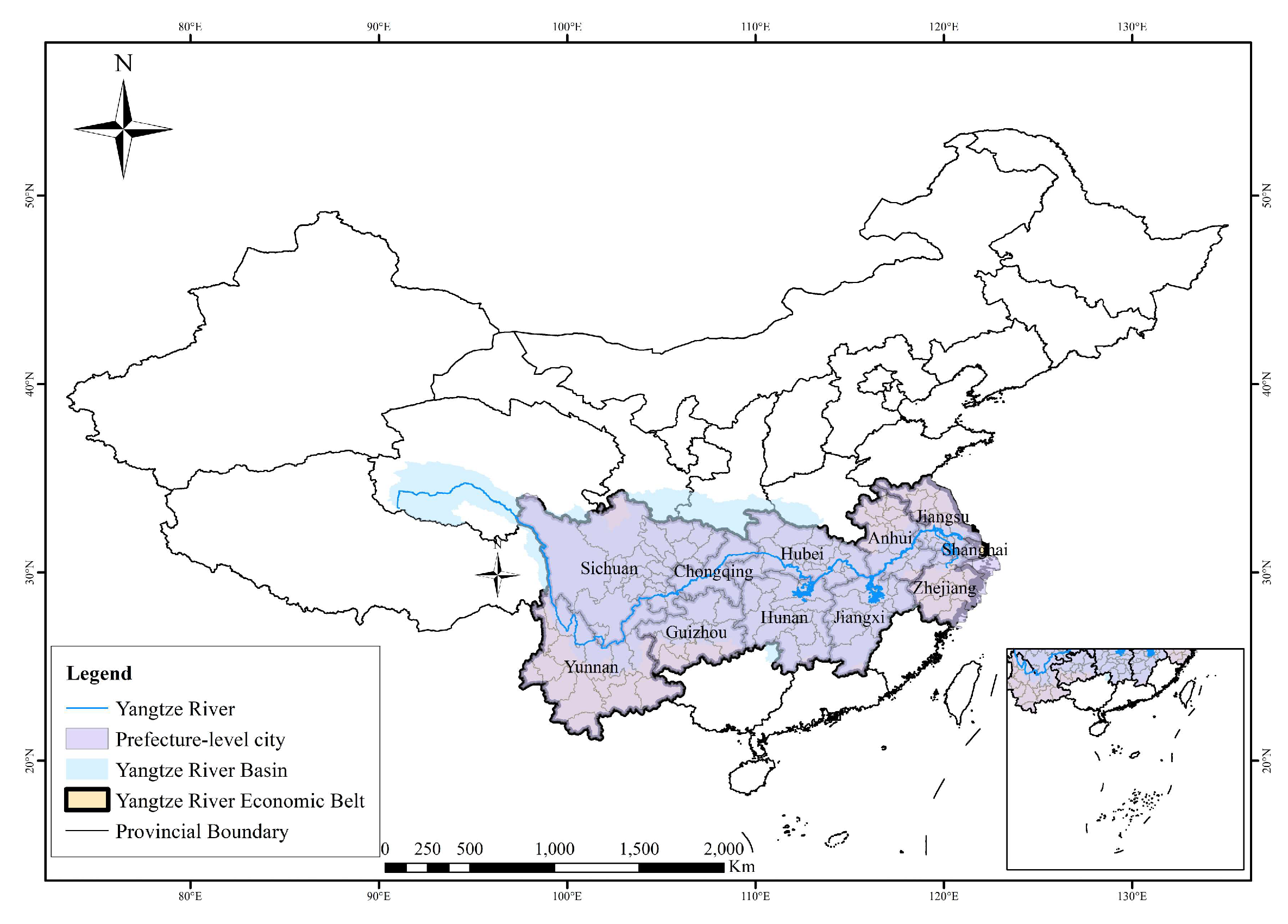
2.1. Study Area and Data

The Yangtze River Economic Belt (97°21′–123°10′ E, 21°08′–35°20′ N), covering an area of 2.05 × 10⁶ km2 with complex topography and elevations above 1000 m, includes three regions (11 provinces) in terms of topography and natural conditions, i.e., the eastern region (Shanghai, Zhejiang, and Jiangsu), the central region (Anhui, Jiangxi, Hubei, and Hunan), and the western region (Sichuan, Chongqing, Yunnan, and Guizhou) (Figure 1) [24]. Specifically, the area can be divided into 126 cities. Taking into account the difficulty of data acquisition, for this study we only selected 110 cities for research. Generally, the Yangtze River Economic Belt is one of China’s three major development strategy areas. With 20% of China’s land area, it supports more than 40% of China’s total economy and contains more than 40% of China’s population [25]. In this study, the data involve six aspects: the water resource endowment, water resource development, water resource utilization, water resource supply and demand, water resource matching, and water resource protection, which can be further divided into 19 indicators (Figure 2). Data for the 11 provinces and 110 cities containing 20 years of water resource data records (from 1999 to 2018) were downloaded from the National Bureau of Statistics (http://www.stats.gov.cn/, accessed on 1 March 2023) and the Water Resources Bulletin for each region (https://swj.sh.gov.cn/szy/, http://jswater.jiangsu.gov.cn/col/col84437/index.html, http://slt.zj.gov.cn/col/col1229243017/index.html, http://slt.ah.gov.cn/tsdw/swj/szyshjjcypj/index.html, https://sjjgl.nit.edu.cn/info/1012/1034.htm, http://slt.hubei.gov.cn/bsfw/cxfw/szygb/, https://slt.hunan.gov.cn/slt/xxgk/tjgb/index.html, http://slt.sc.gov.cn/scsslt/szyzwgk/2022/11/30/19961ab0518840a98c8d52b7163505a4.shtml, http://slj.cq.gov.cn/zwgk_250/fdzdgknr/tjgb/szygb/list.html, http://mwr.guizhou.gov.cn/sjfb/slsj/, http://wcb.yn.gov.cn/html/shuiziyuangongbao/, accessed on 1 March 2023). The datasets are available and have been processed for quality control, with a missing data rate of less than 0.1%. Additionally, for the detailed preliminary data processing methodology readers may refer to the authors’ previous research [2,3].

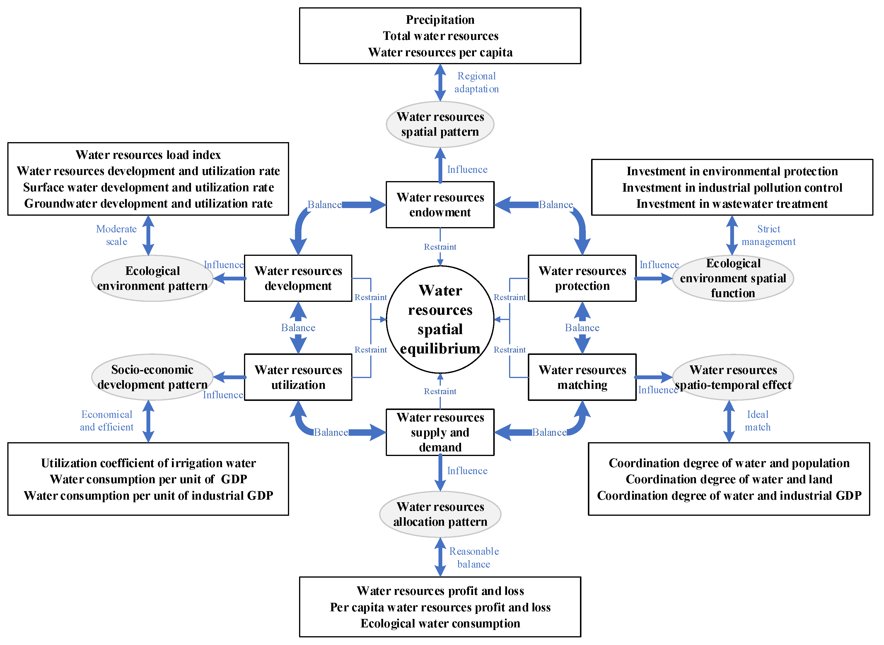
2.2. Conceptual Definition

Research on water resource spatial equilibrium evaluation in China is in its infancy, and scholars have not formed a unified understanding of the related concepts (Table 1). Generally, water resource spatial equilibrium evaluation refers to a relatively stable balance between the development and protection of water resource [26]. This study considers that the key to water resource spatial equilibrium evaluation is to coordinate the relationship between supply and demand of water resource in order to achieve sustainable development. Specifically, this involves six aspects: the water resource endowment, water resource development, water resource utilization, water resource supply and demand, water resource matching, and water resource protection, which can be further divided into 19 indicators [3] (Figure 2).

2.3. Calculation Method

2.3.1. Gini Coefficient

The Gini coefficient was first used to determine whether income distribution is fair, and can provide an objective reflection of the regional income gap [31]. The Gini coefficient is generally between 0 and 1. The closer to 0 it is, the fairer the income distribution. In this study, the relevant conventions and water resource spatial equilibrium are combined to express the classification of water resource spatial equilibrium based on the Gini coefficient (Table 2), and a simple calculation formula is derived to determine the Gini coefficient of the six indexes:
G = 1 1 n 2 i = 1 n 1 y i + 1
where G is the Gini coefficient, y i is the percentage of the sum of each index ( y ) from 1 to i in the total, and n is the total number.

2.3.2. Variable Set

The water resource spatial equilibrium grade is a fuzzy concept, and there is no clear boundary between adjacent grades. Thus, any two adjacent grades can form a group of opposite events; then, all the opposite events are as follows: I and II, II and III, III and IV, IV and V. According to the variable set and the relative membership degree, for a given fixed index there can only be a fuzzy membership relationship with a group of opposite events of adjacent grades [32].
Let the scheme set U = u 1 , u 2 , , u n = u j j = 1 , 2 , n , X i j = x i j i = 1 , 2 , m be each index value of scheme j , and let x i j be the value of index i of scheme j . Index i is divided into five grades, and the interval matrix of the five grades is as follows:
I = a i h , b i h h = 1 , 2 , , 5
where a i h , b i h is the upper and lower limits of index i in the standard value range of grade h .
According to the theorem of the unity of opposites of variable sets, there must be a gradual change point k i h of index i between grade h and grade h + 1 in the interval value of grade h .
k i h = c h c 1 a i h + h 1 c 1 b i h
The matrix K is obtained from k i h and matrix I , where K = k i h , b i h . If the index value of x i j is between two adjacent grades h and h + 1 of matrix K , the relative membership degree of x i j to h is:
μ i h u j = 0.5 1 + b i h x i j b i h k i h x i j k i h , b i h
μ i h u j = 0.5 1 b i h x i j b i h k i h + 1 x i j b i h , k i h + 1
The relative membership degree of index i smaller than h or greater than h + 1 is 0:
μ i ( < h ) u j = 0 , μ i ( > h + 1 ) u j = 0
The comprehensive relative membership degree of each scheme u j to grade h is calculated as follows:
v h u j = i = 1 m w i μ i h u j
where w i is the weight of index i and ω 1 + ω 2 + + ω m = 1 .
The grade characteristic value corresponding to scheme u j is calculated as follows:
H u j = h = 1 c v h 0 u j h
where v h 0 u j is the normalized vector of v h u j .
The characteristic value of each scheme is calculated; the smaller the characteristic value is, the better the scheme.

2.3.3. Set Pair and Partial Connection Number

Considering the dynamics of the water resource system, the set pair analysis method and partial connection number method are used to establish the assessment model of water resource spatial equilibrium. Zhao proposed set pair analysis theory in 1989. It is mainly used to address the uncertainty of systems [33]. The connection number is the core concept of set pair analysis, which is used to address the uncertainty caused by fuzzy, random, intermediary, or incomplete information [34]:
u = a + b i + c j + d k + e l
where 0 a , b , c , d , e 1 , a + b + c + d + e = 1 , taking “+” as the positive direction, and a b c d e .
The spatial equilibrium grade is combined with the five-element connection number. Then, a represents the information component of grade I, b represents the information component of grade II, c represents the information component of grade III, d represents the information component of grade IV, and e represents the information component of grade V.
For the five-element connection number a + b i + c j + d k + e l , its first-order partial positive connective number + u is
+ u = + a + i + b + j + c + k + d
where + a = a a + b , + b = b b + c , + c = c c + d , + d = d d + e .
Its first-order partial negative connective number u is
u = i b + j c + k d + l e
where b = b a + b , c = c b + c , d = d c + d , e = e d + e .
The partial connection number reflects the dynamic trend of the system and determines the evolution rate of the grade. For example, + a reflects the evolution rate from level b to level a . In addition, in this study we only consider the evolution between adjacent levels, that is, we ignore the evolution of leapfrog information.
In the determination of the spatial equilibrium grade, the information component a plays an absolute supporting role for grade I. However, the information component b has an evolutionary trend with respect to to level a ; thus, it is necessary to comprehensively consider the supporting role of b for grade I.
Here, + a is called the support coefficient of the information component b with respect to grade I, and b + a is called the support degree of information component b with respect to grade I, from which the support degree S I of grade I can be obtained:
S I = a + b + a = a + b a a + b
In the same way, the support degrees of II ,   III ,   IV , V can be obtained as follows:
S II = a b + b + c + b = a b a + b + b + c b b + c
S III = b c + c + d + c = b c b + c + c + d c c + d
S IV = c d + d + e + d = c d c + d + d + e d d + e
S V = d e + e = d e d + e + e
S I , S II , S III , S IV , S V are compared and the grades are determined according to the principle of maximum supporting degrees.

2.3.4. Technology Roadmap

The calculation process of the model constructed is as follows (Figure 3).

3. Model Application

Here, the water resource spatial equilibrium is evaluated according to the six selected indexes. Additionally, the water resource development index and water resource utilization index are negative, with smaller values being better. The other four indexes are positive, and larger values are better. To eliminate the influence of dimension, corresponding to the spatial equilibrium grade described in this study, the Gini coefficient is used to standardize the indexes. Then, the indexes after standardization are all negative, and smaller values are better. In calculating the spatial equilibrium, the weight of each index is very important. In this study, we adopt balanced weighting, that is, the weight of each index is the same.

3.1. Calculation of the Grade Characteristic Values Based on the Variable Set

Because all indexes are standardized with the Gini coefficient, all standardized indexes have the characteristics of the Gini coefficient. According to the division standard of the Gini coefficient, the optimal interval matrix of each index is determined as follows:
I = 0 , 0.2 0.2 , 0.3 0.3 , 0.4 0.4 , 0.5 0.5 , 1 0 , 0.2 0.2 , 0.3 0.3 , 0.4 0.4 , 0.5 0.5 , 1 0 , 0.2 0.2 , 0.3 0.3 , 0.4 0.4 , 0.5 0.5 , 1 0 , 0.2 0.2 , 0.3 0.3 , 0.4 0.4 , 0.5 0.5 , 1 0 , 0.2 0.2 , 0.3 0.3 , 0.4 0.4 , 0.5 0.5 , 1 0 , 0.2 0.2 , 0.3 0.3 , 0.4 0.4 , 0.5 0.5 , 1
According to the matrix I and Formula (3), the gradual change point matrix K of the relative membership degree of each index with respect to the five grades is obtained.
K = 0       0.225       0.335     0.475       1 0       0.225       0.335     0.475       1 0       0.225       0.335     0.475       1 0       0.225       0.335     0.475       1 0       0.225       0.335     0.475       1 0       0.225       0.335     0.475       1
According to Formulas (4) and (5), the relative membership degree of the water resource spatial equilibrium is calculated relative to the five grades. Finally, the grade characteristic values can be obtained based on Formula (7) and (8). In this study, we use 2018 as an example to show the calculation process for the 11 provinces (Table 3).

3.2. Determination of the Evaluation Grade Based on Partial Connection Number

According to the relative membership degree of the water resource spatial equilibrium of the 11 provinces in the Yangtze River Economic Belt obtained in Table 3 combined with the five-element connection number, the connection number of the water resource spatial equilibrium of the 11 provinces can be obtained. Using Shanghai as an example, the five-element connection number of the water resource spatial equilibrium in 2018 is as follows.
μ = 0 + 0.06 i + 0.09 j + 0.16 k + 0.69 l
Then, the support degrees for each grade of the water resource spatial equilibrium in Shanghai (2018) are calculated using Formulas (12) to (16).
S I = 0 ,   S II = 0.15 ,   S III = 0.19 ,   S IV = 0.21 ,   S V = 0.82
According to the principle of maximum support degrees, it can be determined that the water resource spatial equilibrium in Shanghai (2018) is grade V. The results for the other provinces are calculated similarly.

4. Results

4.1. Provinces

The grade of the water resource spatial equilibrium gradually improved over time; the spatial distribution trend in the south was better than in the north, and the trend in the west was better than that in the east (Figure 4). In general, the water resource spatial equilibrium of the 11 provinces was sorted as follows: Yunnan > Sichuan > Zhejiang > Jiangxi > Hunan Province > Guizhou > Hubei > Chongqing > Anhui > Jiangsu > Shanghai. The temporal trend could be divided into four stages. Serious disequilibrium occurred 1999 to 2006, with more than two thirds of the provinces were in a state of disequilibrium each year. There was a relative equilibrium state from 2007 to 2008, when Shanghai, Jiangsu, and Anhui were below grade IV. The rebound stage was from 2009 to 2013, when more than two fifths of the provinces were in a state of disequilibrium. Finally, in the improvement stage from 2014 to 2018, only one or two provinces were in disequilibrium.
As a specific example, the water resource spatial equilibrium in Shanghai has generally been poor. Shanghai had grades above V from 1999 to 2018, with the exception of 2016, when it had a grade of IV. The main reason for this pattern is that Shanghai has a large population density and a large demand for water resources. The total water supply is much larger than the total water resources. In the past 20 years, water resources in Shanghai have faced extreme shortages, with an average water deficit of 76.61 × 10⁸ m3/a and per capita water deficit of 382.19 m3/a. Although the local economy is highly developed, the other five indexes are at or near the bottom.
Though the water resource spatial equilibrium in Jiangsu is better than that in Shanghai, the situation is nonetheless severe. From 1999 to 2018, 90% of the grades were in a state of disequilibrium, although the spatial equilibrium grade showed an upward trend, gradually changing from grade V to grade IV. The spatial equilibrium grade even reached grade III in 2015 and grade II in 2016. Similar to the reasons for disequilibrium in Shanghai, over the past 20 years water resource in Jiangsu have faced extreme shortages. The average water deficit is 127.74 × 10⁸ m3/a, and the per capita water deficit is 166.90 m3/a. However, water resource utilization and water resource protection in Jiangsu are basically at the highest level, with the GDP accounting for 22.21% and investment in environmental protection accounting for 23.41% of the total for the Yangtze River economic belt.
The water resource spatial equilibrium in Zhejiang is relatively good. From 1999 to 2018, all grades were all above III except in 2003. In recent years, grade I has even been reached. Zhejiang is rich in total water resources, and the average total water resource is 1028.52 × 108 m3/a, ranking fifth in the Yangtze River Economic Belt. In addition, the per capita water resource is high at 1975.48 m3/a. Zhejiang’s economy is highly developed, the water consumption per unit of GDP has decreased to less than 30 m3, and the water consumption per unit of industrial GDP has reached less than 25 m3. In general, the water resource development index and water resource supply and demand index are at moderate positions, and the other four indexes are better.
There is an obvious turning point in the water resource spatial equilibrium in Anhui, which showed disequilibrium from 1999 to 2013 and equilibrium from 2014 to 2018. Specifically, the utilization coefficient of irrigation water exceeded 0.55, while the water consumption per unit of GDP and the water consumption per unit of industrial GDP both decreased rapidly to below 100 m3 and 80 m3 after 2014. In addition, the investment in environmental protection increased, with its proportion in the Yangtze River Economic Belt increasing from 7.85% in 1999 to 13.05% in 2018. Finally, the water resource utilization index and water resource protection index have significantly improved.
The water resource spatial equilibrium in Jiangxi is relatively good, and there was been no serious disequilibrium from 1999 to 2018. General disequilibrium occurred in early 2001, 2004, and 2005. At other times, the grades were all above relative equilibrium. In recent years, they have basically been in an absolute equilibrium state. The main reason for this is that the water resource utilization index and water resource protection index were the lowest, and the other indexes were relatively superior. This shows that the water resource spatial equilibrium in Jiangxi depends on the natural conditions of the water resource, with economic development being poor.
The water resource spatial equilibrium in Hubei can be divided into two stages: below grade IV from 1999 to 2012 and above grade III from 2013 to 2018. With rapid economic development, Hubei has always been the leader of the central provinces in the Yangtze River Economic Belt. Over the past 20 years, its average GDP has been the fourth highest in the Yangtze River Economic Belt and the highest in the central provinces. In addition, the water consumption per unit of GDP is fifth in the Yangtze River Economic Belt. Furthermore, the intensity of water environmental protection is increasing, being the third highest in the Yangtze River Economic Belt, which promotes the gradual improvement of the overall water resource spatial equilibrium.
The water resource spatial equilibrium in Hunan is good. From 1999 to 2018, except for grade IV in 2001, each year was grade III or below. Additionally, the precipitation in Hunan has increased in recent years, and the total water resource have become larger, accounting for 13.92% in the Yangtze River Economic Belt. The water resource supply and demand have become more secure, and grade I has shown a gradually increasing trend.
The water resource spatial equilibrium in Chongqing shows a clear trend, gradually transforming from grade IV to grade III. This is mainly due to the improvement of water resource development in recent years; the development and utilization rate of water resource is 14.49%, ranking fourth in the Yangtze River Economic Belt.
The water resource spatial equilibrium in Sichuan and Yunnan occupied optimal and suboptimal positions, respectively, with both being below grade II and grade I accounting for 65% and 75% of grades, respectively, over the past 20 years. However, the reasons for this pattern are different for Sichuan and Yunnan. Sichuan performs better on all six indexes, while Yunnan performs poorly on the water resource utilization index and water resources protection index. Specifically, the water consumption per unit of GDP in Sichuan and Yunnan is 46 m3 and 59 m3, respectively.
The water resource spatial equilibrium in Guizhou is distinct, with grade IV from 1999 to 2006, grade III from 2007 to 2013, and grade II from 2014 to 2018. The reason for the continuous improvement in the water resource spatial equilibrium in Guizhou is the same as in Yunnan.
Although the water resource spatial equilibrium in the 11 provinces of the Yangtze River Economic Belt was different from 1999 to 2018, it can be divided into three categories. Shanghai and Jiangsu are economically developed, but have limited water resources; thus, they are always in a state of disequilibrium. Jiangxi, Guizhou, and Yunnan are in the opposite situation; their natural water resource conditions are extremely good, while their socioeconomic development is low and the overall situation is in equilibrium. In the other provinces, the spatial equilibrium grade has been steadily improving due to a medium level of water resources and rapid development of the social economy. Additionally, the evolutionary trend of the water resource spatial equilibrium in the 11 provinces of the Yangtze River Economic Belt is increasing, except in Yunnan, which is due to five cities (Yuxi, Baoshan, Lijiang, Pu’er, and Lincang) having a negative evolutionary trend. However, because the water resource spatial equilibrium in Yunnan is optimal, the water resource spatial equilibrium in the 11 provinces of the Yangtze River Economic Belt has tended to improve from 1999 to 2018.

4.2. Cities

From the perspective of the 110 cities in the Yangtze River Economic Belt, the water resource spatial equilibrium shows that the spatial trend of the three major urban agglomerations is much better than that of the other regions, and that the characteristics of the temporal trend are gradually improving (Figure 5). The temporal trend can be divided into two stages. During the period of steady volatility from 1999 to 2011, approximately 50% of the cities were above grade IV each year. In the next stage, increasing year by year from 2012 to 2018, the proportion of cities above grade IV was only 28.83%. Within the Yangtze River Economic Belt, there is a significant gap in the water resource spatial equilibrium among cities. Based on the natural breaking point analysis method, the 110 cities in the Yangtze River Economic Belt were divided into five categories.
The first category consists of excellent cities, and includes Hangzhou, Wenzhou, Jinhua, Quzhou, Lishui, Xuancheng, Chizhou, Huangshan, Yingtan, Ganzhou, Ji’an, Yichun, Fuzhou, Shangrao, Yichang, Zhuzhou, Shaoyang, Changde, Zhangjiajie, Chenzhou, Yongzhou, Huaihua, Panzhihua, Leshan, Dazhou, Ya’an, Zunyi, Tongren, Baoshan, Lijiang, Pu’er, and Lincang. The water resource spatial equilibrium for these cities was far ahead of that of other cities, and they were all below grade III from 1999 to 2018. In particular, the group of ten cities that includes Quzhou, Lishui, Huangshan, Fuzhou, Shangrao, Huaihua, Baoshan, Lijiang, Pu’er, and Lincang were all below grade II. These cities have excellent performance in terms of their water resource spatial equilibrium, mainly due to their being comprehensively outstanding in all six indexes. These cities have regionally adapted water resource spatial patterns, moderately scaled ecological environmental patterns, efficient economic and socioeconomic development patterns, reasonable and balanced water resource allocation patterns, ideally matched water resource spatiotemporal effects, and strictly managed ecological environmental spatial functions. These regions have certain innovative advantages and early experience in driving the improvement of water resource spatial equilibrium.
The second category consists of good cities, and includes Ningbo, Shaoxing, Taizhou, Anqing, Jingdezhen, Pingxiang, Jiujiang, Huanggang, Shiyan, Xianning, Changsha, Hengyang, Yueyang, Yiyang, Luzhou, Mianyang, Guangyuan, Yibin, Bazhong, Qujing, Yuxi, and Zhaotong. The water resource spatial equilibrium in this type of city is relatively good. While the proportion of cities below grade III from 1999 to 2018 exceeded 75%, the manifestations were different, and were mainly divided into two types. For example, Ningbo is a leading city in the water resource utilization index and water resource protection index, with high water efficiency. The water consumption per unit of GDP and industrial GDP were less than 20 m3 and 25 m3, respectively, and Ningbo is an important model city for environmental protection. Lincang shows good natural water resource conditions, with water resources per capita of 6070.36 m3, which is 2.66 times the national average level. The water resource development range is low, at only 6.51%, and the water resources match well. However, the economic development level is low, and the water consumption per unit of GDP is over 130 m3.
The third category is medium cities, which include Chongqing, Xinyu, Liupanshui, Lu’an, Loudi, Bijie, Huzhou, Nanchang, Anshun, Kunming, Jingzhou, Meishan, and Guiyang. The overall grade of this category of cities is inferior to that of the previous category, though they tend to perform well on certain individual indexes. For example, Kunming has a good water resource utilization index, rapid economic development, and good water efficiency. The water consumption per unit of GDP is 36 m3, ranking 15th among the 110 cities of the Yangtze River Economic Belt. Guiyang has a high water resource protection index, and its investment in environmental protection increased 28.82 times in 2018 compared with 1999. Bijie’s water resource development index is relatively low; the average water resource development utilization rate is only 9.24%, although the inherent condition of water resources is very high.
The fourth category is poor cities, and includes Zhoushan, Chengdu, Wuhan, Huangshi, Xiangtan, Yancheng, Suizhou, Guang’an, Suzhou, and Wuhu. The water resource spatial equilibrium in this type of city is relatively weak. Although there are individual indexes that perform well, the overall situation is not outstanding. For example, Wuhan’s economic development is growing rapidly and its water efficiency is high. The water consumption per unit of GDP and industrial GDP are less than 25 m3 and 30 m3, respectively; however, the water resource per capita is extremely low, with an average of 580.51 m3, which is 28.07% of the national average. Chengdu is similar to Wuhan. Although Chengdu has relatively high investment in environmental protection, the water consumption per unit of GDP and industrial GDP are approximately 100 m3, resulting in low water efficiency.
The fifth category is bad cities, which includes the rest of the cities. The water resource spatial equilibrium in this type of city is extremely weak, and there is a significant gap compared with the other four types of cities. There are two main factors restricting the water resource spatial equilibrium in these cities: first, all six indexes may have shortcomings and not be outstanding in any aspect; second, where an individual index is extremely high, the other indexes are extremely poor. For example, all six indexes are basically at the bottom for Neijiang and Suining; on the other hand, while Shanghai and Nanjing both have high water resource utilization indexes, on the other five indexes they are at or near the bottom.
Additionally, the evolutionary trend of water resource spatial equilibrium is increasing in the 110 cities except for Huanggang, Luzhou, Neijiang, Yuxi, Baoshan, Lijiang, Pu’er, and Lincang (Figure 6).

5. Discussion

5.1. Calculation Method of Water Resource Spatial Equilibrium

The water resource spatial equilibrium can be studied from three levels. The first is to only consider the spatial equilibrium of the water resource system itself, that is, the spatial equilibrium of water resource distribution. For example, the spatial equilibrium of precipitation or water resources quantity can be used to analyze the water resource spatial equilibrium. The second is between two systems (i.e., water resource system and socio-economic system or water resource system and ecological environment system), that is, the spatial equilibrium of the water resource supply and demand is the spatial equilibrium of the water resource supply and demand sides, which can be used to study the spatial matching and coordination relationship of the supply and demand factors. The third is the spatial equilibrium of water resource allocation patterns among the three systems (water resource system, socio-economic system, and ecological environment system). This can be understood as the spatial equilibrium between all factors related to water resources, which can be used to study the structure, combination, and optimization of the entire system in terms of the spatial equilibrium. The key to studying water resource spatial equilibrium is to calculate the coefficient of the water resource spatial equilibrium. There are many methods that can be used to calculate the coefficient of spatial equilibrium. Most existing studies use the inequality relationship to calculate the spatiotemporal equilibrium of the research object; such methods include the Theil index [19], Gini coefficient [20], Lorentz curve [21], and more. However, these static spatial equilibrium coefficients are insufficient to describe the dynamics and ambiguities of a water resource system. In addition to being a complex dynamic system, a water resource system is an unclear fuzzy system. To study and evaluate the water resource spatial equilibrium, it is necessary to consider the dynamic evolution of information and the unity of opposites among different levels. Based on commonly used calculation methods, in this study we have sought to build a new water resource spatial equilibrium evaluation model by combining variable sets and partial connection numbers to effectively compensate for the lack of traditional methods that consider fuzzy indices and dynamic information.

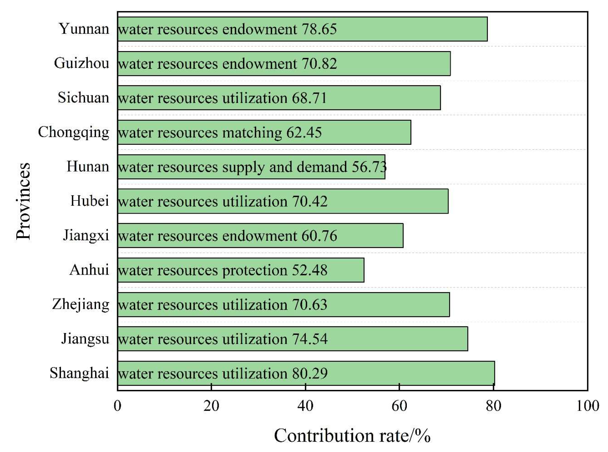
5.2. Factors That Influence Water Resource Spatial Equilibrium

In early influential factor studies of water resource spatial equilibrium, the Gini coefficient and Lorentz curve were the main methods [34]. By calculating the matching degree of water resources, the matching degree between water resources and socio-economic development, and the matching degree between water resources and the ecological environment, a complete analysis and identification process can be formed. At present, the contribution rate method is widely used for the identification of influencing factors thanks to its ability to address uncertainties in multifactor joints [3]. Many studies have analyzed influencing factors in other research fields, such as drought events [3] and food–energy–water [35] conditions. In this study, we suggest that identification of the influencing factors should start from the inherent concept of water resource spatial equilibrium and the mechanisms of each subsystem in order to identify the key factors affecting water resource spatial equilibrium. After calculating the influencing factors of water resource spatial equilibrium in the 11 provinces of the Yangtze River Economic Belt, we found that they can be generally divided into three categories (Figure 7). The first is the water resource endowment, which includes Jiangxi, Guizhou, and Yunnan. The second is water resource utilization, which includes Shanghai, Jiangsu, Zhejiang, Hubei, and Sichuan. The third is other factors, which includes water resource matching in Chongqing, water resource supply and demand in Hunan, and water resource protection in Anhui. These results are not completely consistent with those of Hong [34] and Zuo [26], who stated that population, GDP, land area, and precipitation are the four most important factors. The main reason for this is the different interpretations of the conceptual definition of water resource spatial equilibrium. However, all results agree that economic factors have a large influence.

5.3. Scale Characteristics of Water Resource Spatial Equilibrium

It is of great significance to identify areas with poor water resource spatial equilibrium for future water resource management and optimal allocation [31]. However, there is no research identifying the key areas of water resource spatial equilibrium. Relevant studies in other fields show that the smaller the spatial scale is, the more accurate the identification of key areas. For example, for anthropogenic nitrogen input (NANI), research at the city scale can more effectively identify key pollution areas compared with research at the provincial scale, and the administrative area can be reduced by 23.2% [36]. Comparing the results of water resource spatial equilibrium at the province scale and city scale, in this study we found that when the control targets are set to 20%, 40%, 60%, and 80%, at the provincial level it is necessary to control 7.72%, 21.82%, 38.81%, and 64.12%, respectively, of the administrative area, while at the city level it is only necessary to control 6.53%, 16.82%, 28.29%, and 45.07%, respectively (Figure 8), which is a respective decrease of 1.20%, 4.99%, 10.52%, and 19.05%. Generally, city-scale research on water resource spatial equilibrium can more effectively identify and optimize the control area compared with the provincial scale.

6. Conclusions

In this study, we have proposed a new water resource spatial equilibrium evaluation model that can determine the spatiotemporal characteristics and evolutionary trends of water resource spatial equilibrium. The Yangtze River Economic Belt was used as the study area. From this study, the following conclusions were obtained:
(1)
The water resource spatial equilibrium is used to coordinate the relationship between supply and demand of water resource to achieve the sustainable development.
(2)
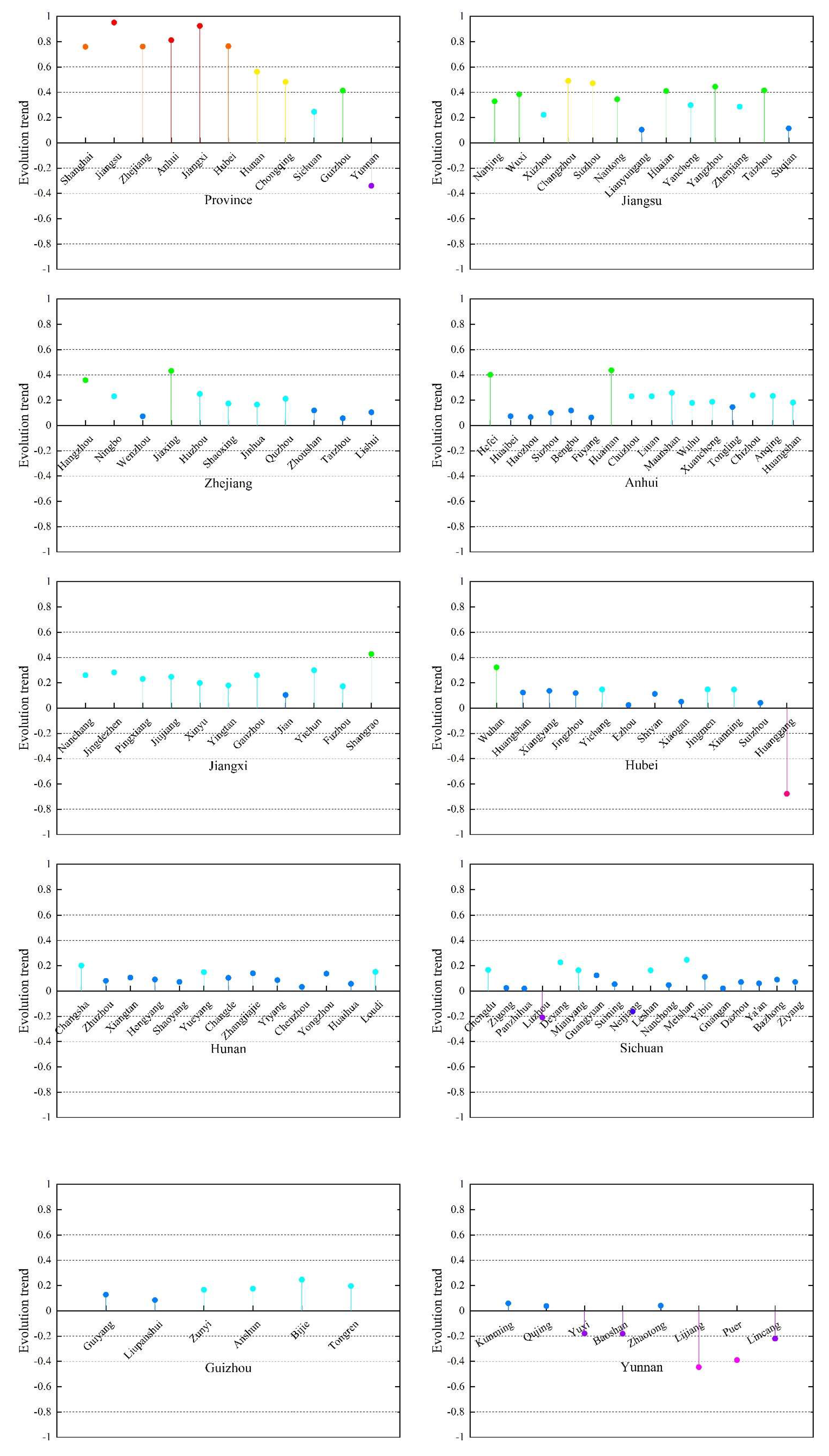
In the 11 provinces of the study area, the water resource spatial equilibrium gradually improved over time. In terms of the spatial trend, the south was better than the north and the west was better than the east. The water resource spatial equilibrium in the 11 provinces was sorted as follows: Yunnan > Sichuan > Zhejiang > Jiangxi > Hunan Province > Guizhou > Hubei > Chongqing > Anhui > Jiangsu > Shanghai.
(3)
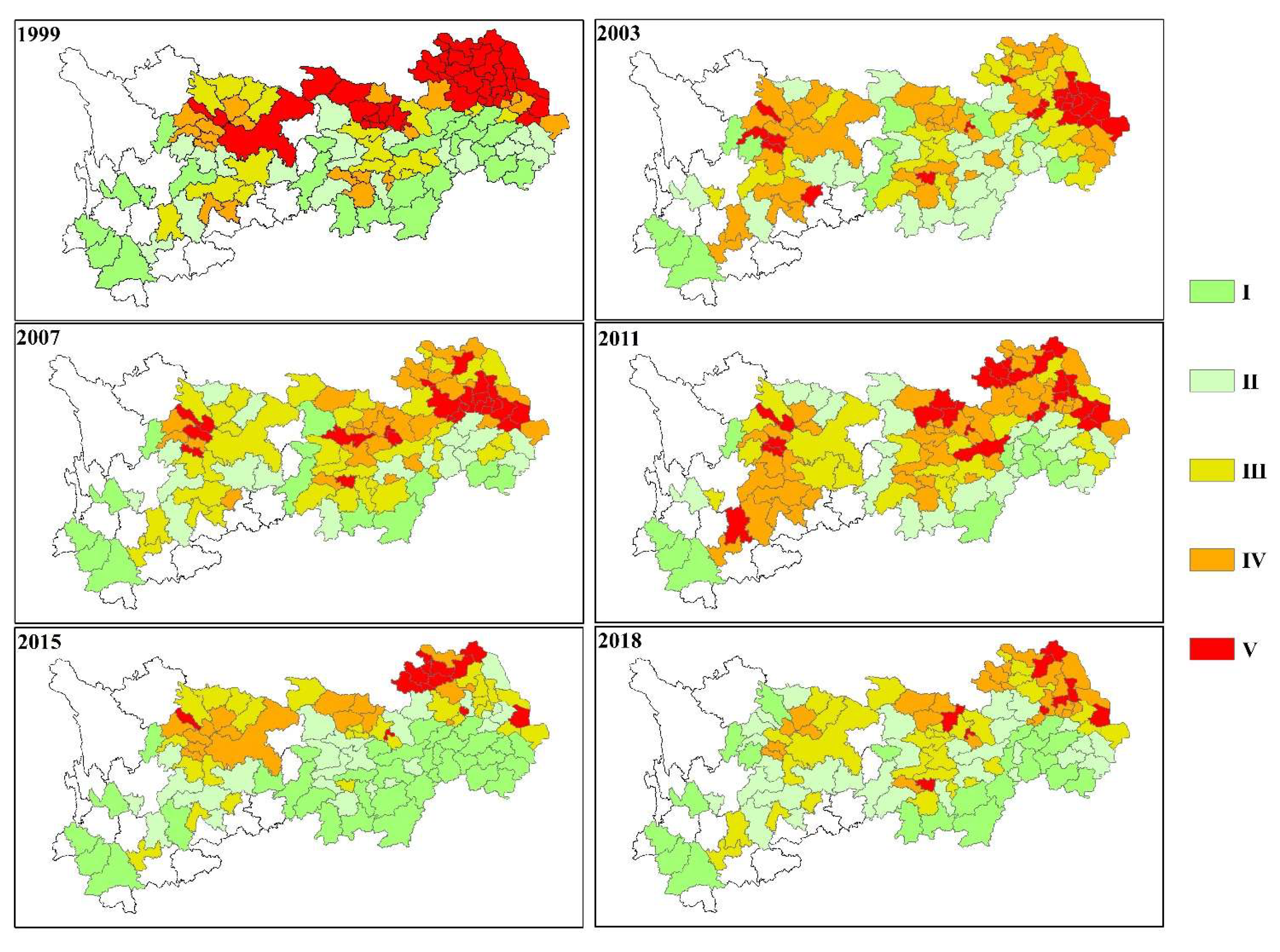
In the 110 cities in the study area, the water resource spatial equilibrium showed that the spatial trend of the three major urban agglomerations was much better than that of the other regions. The temporal trend could be divided into two stages, namely, a stable fluctuation stage from 1999 to 2011 and an improvement stage from 2012 to 2018. The evolutionary trend of water resource spatial equilibrium increased in all cities except Huanggang, Luzhou, Neijiang, Yuxi, Baoshan, Lijiang, Pu’er, and Lincang.
(4)
Compared with the provincial scale, city-scale research on the water resource spatial equilibrium can more effectively identify and optimize the control area. When the control targets were set to 20%, 40%, 60%, and 80%, the proportion of administrative area based on the city scale decreased by 1.20%, 4.99%, 10.52%, and 19.05%, respectively.

Author Contributions

Z.Z. prepared the conceptualization, methodology, validation, data curation, data interpretation, and writing. Y.C. prepared the conceptualization and data curation. Y.Y. prepared the data curation and data interpretation. All authors have seen and approved the manuscript and have contributed significantly to the paper. All authors have read and agreed to the published version of the manuscript.

Funding

This research was supported by the Qin Chuangyuan high-level innovation and entrepreneurship talent project (QCYRCXM-2022-242).

Data Availability Statement

Data available on request from the authors.

Acknowledgments

The authors would like to thank the editors and the anonymous reviewers for their crucial comments, which helped to improve the quality of this paper.

Conflicts of Interest

The manuscript has not been published elsewhere, and it has not been submitted simultaneously for publication elsewhere. We have no conflicts of interest to disclose.

References

  1. Zuo, Q.; Han, C.; Ma, J. Application Rules and Quantification Methods of Water Resources Spatial Equilibrium Theory. Hydro-Sci. Eng. 2019, 6, 50–58. [Google Scholar]
  2. Zhao, Z.; Wang, H.; Zhang, L.; Liu, X.; Zhao, Y. Construction and application of resilience evaluation model of water resource-water environment-social economy complex system in the Yangtze River Economic Belt. Adv. Water Sci. 2022, 33, 705–717. [Google Scholar]
  3. Yang, Y.; Gong, S.; Wang, H.; Zhao, Z.; Yang, B. New model for water resources spatial equilibrium evaluation and its application. Adv. Water Sci. 2021, 32, 33–44. [Google Scholar]
  4. Fox, K.A. A Spatial Equilibrium Model of the Livestock-Feed Economy in the United States. Econ. J. Econ. Soc. 1953, 21, 547–566. [Google Scholar] [CrossRef]
  5. Glaeser, E.L.; Gottlieb, J.D. The Wealth of Cities: Agglomeration Economies and Spatial Equilibrium in the United States. J. Econ. Lit. 2009, 47, 983–1028. [Google Scholar] [CrossRef]
  6. Kawaguchi, T.; Suzuki, N.; Kaiser, H.M. A Spatial Equilibrium Model for Imperfectly Competitive Milk Markets. Am. J. Agric. Econ. 1997, 79, 851–859. [Google Scholar] [CrossRef]
  7. Killingback, T.; Doebeli, M. Spatial Evolutionary Game Theory: Hawks and Doves Revisited. Proc. R. Soc. London. Ser. B Biol. Sci. 1996, 263, 1135–1144. [Google Scholar]
  8. Roca, C.P.; Cuesta, J.A.; Sánchez, A. Evolutionary Game Theory: Temporal and Spatial Effects beyond Replicator Dynamics. Phys. Life Rev. 2009, 6, 208–249. [Google Scholar] [CrossRef]
  9. Bhattacharjee, A.; Maiti, T.; Petrie, D. General Equilibrium Effects of Spatial Structure: Health Outcomes and Health Behaviours in Scotland. Reg. Sci. Urban Econ. 2014, 49, 286–297. [Google Scholar] [CrossRef]
  10. Wang, J.; Jiao, J.; Chao, D.U.; Hao, H.U. Competition of Spatial Service Hinterlands between High-Speed Rail and Air Transport in China: Present and Future Trends. J. Geogr. Sci. 2015, 25, 1137–1152. [Google Scholar] [CrossRef]
  11. Fan, X.; Ying, C.; Ming, D.; Yuping, H. Calculation method and application of spatial equilibrium coefficient of water resources. Water Resour. Prot. 2020, 36, 52–57. [Google Scholar]
  12. Chao, C.; Shaoyu, T.; Haiying, P.; Shaokai, Y. Ecological carrying capacity of water resources in the central Yunnan urban agglomeration area. Resour. Sci. 2016, 38, 1561–1571. [Google Scholar] [CrossRef]
  13. Dai, J.; Ji, C. An Competition Equilibrium Model on the Diverse-Source Water Supply Market Created by Interbasin Water Transfer. In Proceedings of the 2006 International Conference on Management Science and Engineering, Lille, France, 5–7 October 2006; Zhang, H., Zhao, R.M., Chen, L., Eds.; Curran Associates, Inc.: New York, NY, USA, 2006; pp. 995–1000. [Google Scholar]
  14. Wang, J.F.; Liu, C.M.; Wang, Z.Y.; Yu, J.J. A Marginal Revenue Equilibrium Model for Spatial Water Allocation. Sci. China Ser. D-Earth Sci. 2002, 45, 201–210. [Google Scholar] [CrossRef]
  15. Shi, W.; Yu, X.; Liao, W.; Wang, Y.; Jia, B. Spatial and Temporal Variability of Daily Precipitation Concentration in the Lancang River Basin, China. J. Hydrol. 2013, 495, 197–207. [Google Scholar] [CrossRef]
  16. De, L.M.; González-Hidalgo, J.C.; Brunetti, M.; Longares, L.A. Precipitation Concentration Changes in Spain 1946–2005. Nat. Hazards Earth Syst. Sci. 2011, 11, 1259–1265. [Google Scholar] [CrossRef]
  17. Coscarelli, R.; Caloiero, T. Analysis of Daily and Monthly Rainfall Concentration in Southern Italy (Calabria Region). J. Hydrol. 2012, 416–417, 145–156. [Google Scholar] [CrossRef]
  18. Vyshkvarkova, E.; Voskresenskaya, E.; Martin-Vide, J. Spatial Distribution of the Daily Precipitation Concentration Index in Southern Russia. Atmos. Res. 2018, 203, 36–43. [Google Scholar] [CrossRef]
  19. Monjo, R.; Martin-Vide, J. Daily Precipitation Concentration around the World According to Several Indices. Int. J. Climatol. 2016, 36, 3828–3838. [Google Scholar] [CrossRef]
  20. Zhou, R.; Jin, J.; Cui, Y.; Ning, S.; Zhou, L.; Zhang, L.; Wu, C.; Zhou, Y. Spatial Equilibrium Evaluation of Regional Water Resources Carrying Capacity based on Dynamic Weight Method and Gagum Gini Coefficient. Front. Earth Sci. 2022, 9, 790349. [Google Scholar] [CrossRef]
  21. Xingmin, S.; Wenjuan, W. Gini Coefficient of Ecological Security of Shaanxi Based on Water Resources. Agric. Res. Arid Areas 2010, 28, 233–236. [Google Scholar]
  22. Xiaoya, Z.; Shilun, Y. Climatic and Anthropogenic Impacts on Water Discharge in the Yangtze River Over the Last 56 Years (1956–2011). Resour. Environ. Yangtze Basin 2014, 23, 1729–1739. [Google Scholar]
  23. Liu, B.; Jiang, T.; Ren, G.; Fraedrich, K. Projected Surface Water Resource of the Yangtze River Basin Before 2050. Clim. Chang. Res. 2007, 3, 145–150. [Google Scholar]
  24. Peng, M.; Xu, H.; Qu, C.; Xu, J.; Chen, L.; Duan, L.; Hao, J. Understanding China’s Largest Sustainability Experiment: At-mospheric and Climate Governance in the Yangtze River Economic Belt as a Lens. J. Clean. Prod. 2021, 290, 125760. [Google Scholar] [CrossRef]
  25. Kong, Y.; He, W.; Yuan, L.; Zhang, Z.; Gao, X.; Zhao, Y.; Degefu, D.M. Decoupling Economic Growth from Water Consumption in the Yangtze River Economic Belt, China. Ecol. Indic. 2021, 123, 107344. [Google Scholar] [CrossRef]
  26. Zuo, Q.; Han, C.; Ma, J.; Wang, X. Theoretical Method and Applied Research Framework of Water Resources Spatial Equilib-rium. Yellow River 2019, 41, 113–118. [Google Scholar]
  27. Wang, H.; Liu, J. Collaboration of National Water Resources with Eco-Social System in China. China Water Resour. 2016, 17, 7–9. [Google Scholar]
  28. Jin, J.; Li, J.; Wu, C. Research Progress on Spatial Equilibrium of Water Resources. J. North China Univ. Water Resour. Electr. Power (Nat. Sci. Ed.) 2019, 40, 47–60. [Google Scholar]
  29. Wang, J. Implement “Spatial Equilibrium” to Strengthen the Rigid Constraints of Carrying Capacity. Water Resour. Dev. Res. 2018, 18, 20–21. [Google Scholar]
  30. Li, J.; Wang, P.; He, J.; Guo, X. Study on Theory Methodology and Countermeasures about Water Resources Spatial Equilibrium. China Water Resour. 2019, 23, 23–25. [Google Scholar]
  31. Flinn, J.; Guise, J. An Application of Spatial Equilibrium Analysis to Water Resource Allocation. Water Resour. Res. 1970, 6, 398. [Google Scholar] [CrossRef]
  32. Chen, S. Theory and Model of Engineering Variable Fuzzy Set—Mathematical Basis for Fuzzy Hydrology and Water Re-sources. J. Dalian Univ. Technol. 2005, 2, 308–312. [Google Scholar]
  33. Liu, X.; Zhao, K. Multiple Attribute Decision Making and Its Applications Based on Complex Number Arithmetic Operation of Connection Number with Interval Numbers. Math. Pract. Theory 2008, 38, 57–64. [Google Scholar]
  34. Hong, S.; Song, Z.; Cheng, T.; Wang, H. Spatial Matching Analysis of Water Resources in the Intake Area of South-North Water Transfer Project Based on Gini Coefficient. J. Beijing Norm. Univ. (Nat. Sci.) 2017, 53, 175–179. [Google Scholar]
  35. Deng, C.; Wang, H.; Gong, S.; Zhang, J.; Yang, B.; Zhao, Z. Effects of Urbanization on Food-Energy-Water Systems in Mega-Urban Regions: A Case Study of the Bohai MUR, China. Environ. Res. Lett. 2020, 15, 044014. [Google Scholar] [CrossRef]
  36. Wei, G.; Huaicheng, G.; Xikang, H. Evaluating City-Scale Net Anthropogenic Nitrogen Input (NANI) in Mainland China. Acta Sci. Nat. Univ. Pekin. 2014, 50, 951–959. [Google Scholar]
Figure 1. Location of the administrative division of the Yangtze River Economic Belt.
Water 15 02984 g001
Figure 2. Schematic diagram of water resource spatial equilibrium.
Water 15 02984 g002
Figure 3. Technology roadmap of this study.
Water 15 02984 g003
Figure 4. The water resource spatial equilibrium in the 11 provinces.
Water 15 02984 g004
Figure 5. The water resource spatial equilibrium in the 110 cities.
Water 15 02984 g005
Figure 6. The evolutionary trend of water resource spatial equilibrium in the 11 provinces and 110 cities.
Water 15 02984 g006
Figure 7. The contribution rate of water resource spatial equilibrium in the 11 provinces.
Water 15 02984 g007
Figure 8. The proportion of administrative area to different control targets at the provincial scale and city scale.
Water 15 02984 g008
Table 1. The conceptual definition of water resource spatial equilibrium.
ScholarDefinition
Wang [27]Coordinated development among water resource carrying capacity, socioeconomic systems, and different regions.
Zuo [26]A relatively stable and balanced state of development, utilization, and protection of water resource in space.
Jin [28]The water resource spatial equilibrium is a dual balance of supply and demand of water resources, which is coordinated and matched in time and space among the water resource spatial distribution, social economy, and ecological environment.
Wang [29]The population and economy is balanced with the water resource carrying capacity, in which people and water live in harmony.
Li [30]The population, economic, and social development of a river basin or a certain area is balanced with water resources.
Table 2. Classification of water resource spatial equilibrium based on the Gini coefficient.
GradeGini Coefficient IntervalIncome DistributionWater Resource Spatial Equilibrium
I0–0.2Absolute averageAbsolute equilibrium
II0.2–0.3General fairnessGeneral equilibrium
III0.3–0.4Relative reasonableRelative equilibrium
IV0.4–0.5General gapGeneral disequilibrium
V0.5–1Great disparitySerious disequilibrium
Table 3. The relative membership degree and grade characteristic values of the 11 provinces in 2018.
DistrictRelative Membership DegreeGrade Characteristic Values
IIIIIIIVV
Shanghai00.060.090.160.694.54
Jiangsu00.050.110.740.203.67
Chongqing00.060.580.280.083.25
Hubei0.020.150.460.3703.19
Anhui0.040.200.520.2402.94
Guizhou00.190.620.1902.88
Hunan0.020.150.700.1302.86
Jiangxi00.240.76002.82
Zhejiang00.790.21002.21
Sichuan0.080.750.17002.07
Yunnan0.320.650.03001.84
Disclaimer/Publisher’s Note: The statements, opinions and data contained in all publications are solely those of the individual author(s) and contributor(s) and not of MDPI and/or the editor(s). MDPI and/or the editor(s) disclaim responsibility for any injury to people or property resulting from any ideas, methods, instructions or products referred to in the content.

