A Dimension-Reduced Line Element Method for 3D Transient Free Surface Flow in Porous Media

Abstract

In order to reduce the numerical difficulty of the 3D transient free surface flow problems in porous media, a line element method is proposed by dimension reduction. Different from the classical continuum-based methods, homogeneous permeable pores in the control volume are conceptualized by a 3D orthogonal network of tubes. To obtain the same hydraulic solution with the continuum model, the equivalent formulas of flow velocity, continuity equation and transient free surface boundary are derivable from the principle of flow balance. In the solution space of transient free surface flow, the 3D problem is transformed into 1D condition, and then a finite element algorithm is simply deduced. The greatest advantage of the line element method is line integration instead of volume/surface integration, which has dramatically decreased the integration difficulty across the jump free surface. Through the analysis of transient free surface flow in the unconfined aquifer, trapezoidal dam, sand flume and wells, the transient free surface locations predicted from the proposed line element method generally agree well with the analytical, experimental and other numerical data in the available literatures, the numerical efficiency can also be well guaranteed. Furthermore, the hydraulic anisotropy has significant effect on the evolution of free surface locations and the shape of depression cones in spatial. The line element method can be expanded to model the 3D unsaturated seepage flow, two-phase flow and thermos problems in porous media because of the similarity between the similarity of Darcy’s law, Buckingham Law and Fourier’s law.

1. Introduction

Transient free surface seepage problems are prevalent in the reservoir–dam system and have a significant effect on the landslide risk in the reservoir and dam stability [1,2,3,4,5]. Due to the indeterminacy of the free surface and seepage boundary over time, the analytical solutions are limited to the homogeneous, isotropic media with simple geometry [6,7,8]. Alternatively, the continuum-based numerical methods have been extensively used to solve the transient free surface seepage problems.

In the early stage, Neuman and Witherspoon [9] proposed a finite element method for unsteady free surface flow in porous media, but the element updates near the moving free surface were required in each timestep. In order to avoid the adaptive mesh updates, a residual flow method with fixed mesh was developed by Desai et al. [10] and verified by the consistency with the available closed-form solution and measured data in a trapezoidal dam. To solve the transient seepage problems with the complicated drainage system, Chen et al. [11] established a parabolic variational inequality method by transferring the moving free surface and seepage boundaries into natural boundaries. Its feasibility was illustrated by the agreements with the in situ monitoring data of an underground powerhouse. To reduce the high cost of mesh generation in the finite element methods, Rafiezadeh and Ataie-Ashtiani [12] presented a boundary element method to model transient seepage flow in both isotropic and anisotropic media with only boundary mesh, whereas the free-surface nodes still needed to be repositioned in each timestep. Moreover, there are some other alternative methods for numerical solutions of transient free surface flow in porous media, such as the finite volume method [13,14], numerical manifold method [15] and so forth. In the above methods, both the pores and grains in the porous media were treated as a homogeneous continuum. In nature, the pores are the occurrence space and flow paths of groundwater rather than solid grains. However, it is quite difficult to capture the flow process of numerous pores. Thus, irregular pore flow is conceptualized as a 3D homogeneous flow through the whole domain of the porous media based on the representative elementary volume (REV, [16]). Alternatively, in the equivalent pipe network model [17,18,19,20] or line element model [21,22] the homogeneous flow through the whole porous media was replaced by 1D pipe/line flow, in which the high-dimensional seepage flow problems were reduced to a lower-dimensional form in solution space, and the computational cost was substantially decreased for memory storage and numerical iteration. Moreover, these approaches provided a method of dimensional reduction to deal with the seepage flow problems through the fractured rock [23,24]. The equivalent pipe network model (PNM) or line element model (LEM) was powerful in analyzing the confined and unconfined, steady and transient seepage flow in 2D isotropic and anisotropic media.

To the best of authors’ knowledge, previous LEMs are limited in the 2D porous media, and the 3D transient free surface flow in porous media has not been addressed yet. In reality, the 3D transient free surface flow is more practical than the 2D condition. Nevertheless, the surface integration across the jump free surface in the continuum-based methods is very complicated. Firstly the polygon shape and spatial plane of the free surface intersected with the tetrahedron/hexahedron elements need to be confirmed. Then, the contribution of flow exchange in the matrix with the specific yield is calculated by triangulating the polygon, which highly depends on the locations of free surface and Gaussian points of triangular subdivision [11]. Therefore, the previous numerical methods including the continuum-based model and PNM/LEM are mainly concentrated in 2D flow conditions and generally mesh-dependent, which may lead to great mathematical difficulty and computational cost in dealing with dynamic free surface. In order to reduce the numerical difficulty and enhance the numerical stability in transient free surface flow in porous media, a line element method is established in this study through dimensional reduction, and the 3D transient free surface flow problem is transformed into a 1D numerical solution space, in which the mesh preparation and line integral with dynamic free surface become quite simple. Firstly, the governing equations and boundary conditions of the 3D transient free surface flow in the porous media are described in mathematics. Secondly, the line element model is proposed with dimension reduction, and a simple finite line element algorithm is developed. Thirdly, the proposed numerical model is verified through comparisons with the unconfined aquifer, trapezoidal dam, sand flume and well.

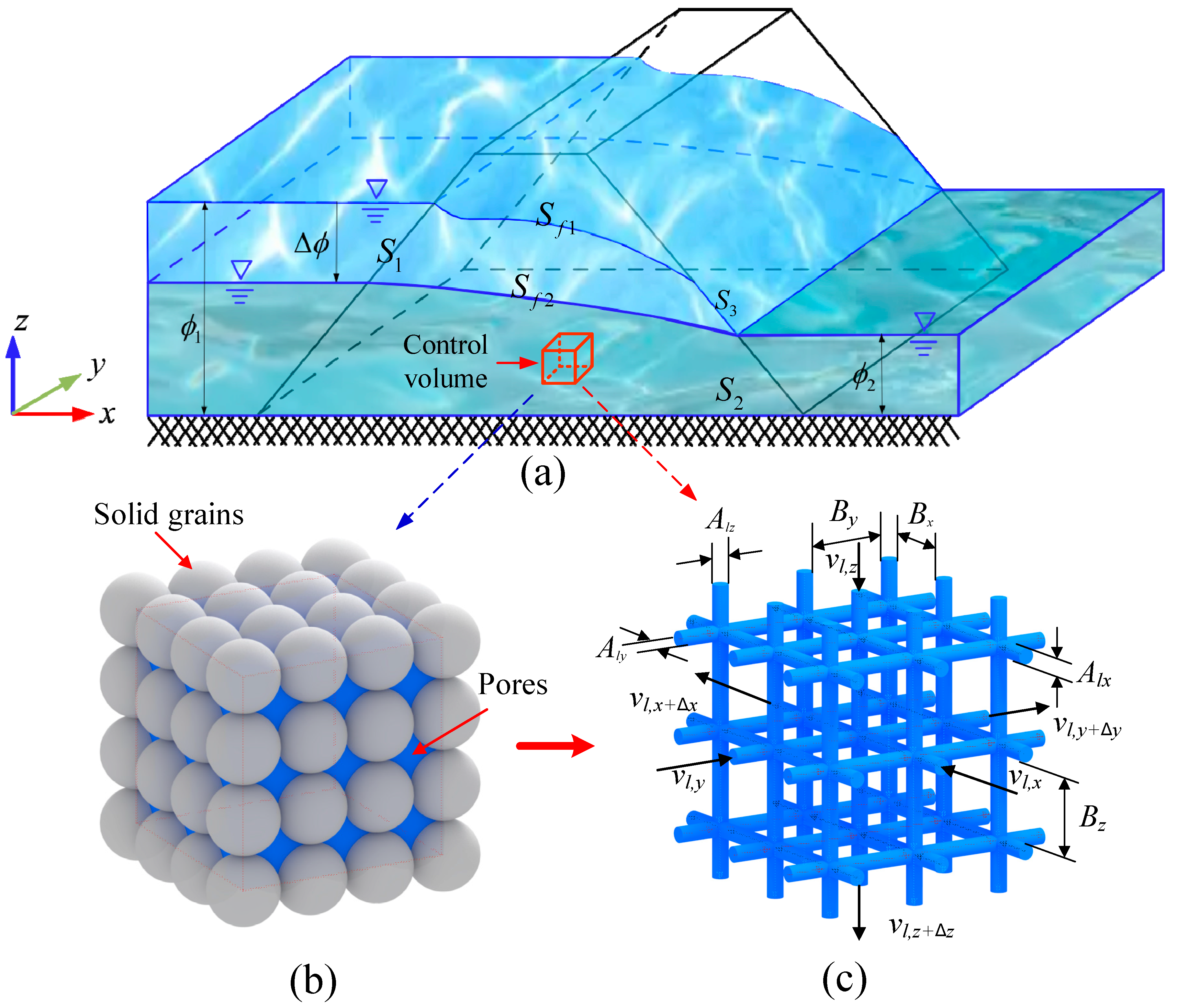
2. Governing Equations

When the water level of upstream reservoir suddenly descends from ${\varphi }_1$ to ${\varphi }_2$, as shown in Figure 1, the free surface in the 3D soil dam will gradually decrease from $S_{f1}$ to $S_{f2}$ over time. In general, the averaged flow velocity through the control volume below the free surface is given by Darcy’s law [16] as

$$\left\{\begin{array}{l}{v}_x=-k_x\partial \varphi /\partial x\\ v_y=-k_y\partial \varphi /\partial y\\ v_z=-k_z\partial \varphi /\partial z\end{array}\right.$$

(1)

where v is the velocity of seepage flow (LT⁻¹), k is the hydraulic conductivity (LT⁻¹), and $\varphi$ is the potential head (L). Note that x, y and z denote the three principal axes of hydraulic conductivity.

During the discharge process, the relationship between the net flow through the surface areas and the rate of change of water amount in the control volume can be given by the following continuity equation [10,11]:

$$-\left(\frac{\partial v_x}{\partial x}+\frac{\partial v_y}{\partial y}+\frac{\partial v_z}{\partial z}\right)=S_s\frac{\partial \varphi }{\partial t}$$

(2)

where S_s is the specific storage (L⁻¹) as the water volume released from a unit soil volume per unit declines in potential head [16], which is determined by the compressibility of solid skeleton and water. Generally, the water release as a result of the specific storage can be ignored in comparison to that of the gravitational specific yield. Thus, Equation (2) is reduced to

$$\frac{\partial v_x}{\partial x}+\frac{\partial v_y}{\partial y}+\frac{\partial v_z}{\partial z}=0$$

(3)

Although the above equation is identical to the continuity equation of the steady free surface flow [25], the distribution of the potential head $\varphi$ subject to the transient free surface is a function of space and time, which is different from the solution of the steady flow as it is only dependent on space. Meanwhile, the transient flow process should also satisfy the initial condition and boundary conditions below:

(1)

The initial condition [11]

$${\left.\varphi \left(x,y,z,t\right)\right|}_{t=0}={\varphi }_0\left(x,y,z\right)$$

(4)

(2)

The potential head boundary S₁ [11]

$$\varphi \left(t\right)=\overline{\varphi }\left(t\right)$$

(5)

where the overline represents prescribed value, and S₁ denotes the flow boundaries below the upstream and downstream water levels and are valued by the given water heads ${\overline{\varphi }}_1\left(t\right)$ and ${\overline{\varphi }}_2\left(t\right)$, respectively.

(3)

The flux boundary S₂ [11]

$$q_n=-\left(v_x{n}_x+v_y{n}_y+v_z{n}_z\right)={\overline{q}}_n\left(t\right)$$

(6)

where n denotes the unit normal vector. As shown in Figure 1a, the base of the soil dam is impervious, and its flux is equal to zero.

(4)

The Signorini-type seepage boundary S₃

Excluding the potential head and flux boundaries, the remaining potential seepage boundary can be divided into two sections: the upper part above the transient free surface S_3u with $\varphi \left(t\right)\le z,q_n\left(t\right)=0$ and the lower part below the transient free surface S_3l with $\varphi \left(t\right)=z,q_n\left(t\right)\le 0$. Thus, the boundary condition on the potential seepage face can be unified as [11]

$$\left\{\begin{array}{l}\varphi \left(t\right)\le z,q_n\left(t\right)\le 0\\ \left[\varphi \left(t\right)-z\right]q_n\left(t\right)=0\end{array}\right.$$

(7)

(5)

The transient free surface boundary $S_f$

Besides the zero-pressure condition $\varphi =z$, the flow exchange through the transient free surface can be calculated as [11]

$$q_n\left(t\right)=-\mu \frac{\partial \varphi }{\partial t}\cos \theta$$

(8)

where μ is the specific yield, and θ is the angle between the outward normal line of the free surface and the upwards vertical line.

3. The Line Element Method

3.1. Equivalent Flow Velocity and Hydraulic Conductivity

The porous media in micro scale is composed of countless solid grains and pores, and the calculative scale is very great if the Navier–Stokes equations are applied on a huge number of pores. Instead, the porous media can be averaged as a continuum using the concept of REV, where the macro hydraulic property performs stably with various sample sizes. However, this assumption contradicts to the fact that the grains cannot conduct water, with the exception of the pores. Conversely to the traditional continuum model, the homogeneous porous medium can be seen as the combination of regular arrayed spherical grains, as shown in Figure 1b. Due to the similarity of flow property between the pore and tube [26,27,28], the permeable pores between the solid grains in the x, y and z directions are conceptualized by a 3D orthogonal network of tubes, as shown in Figure 1c. For simplicity, the tube is represented by the line element in this study.

To ensure solution equivalence between the line element model and continuum model, these two models should have identical distributions of potential head and hydraulic gradient in the 3D space. Therefore, the flow velocity through the line elements can be expressed in the form of Darcy’s law:

$$\left\{\begin{array}{l}{v}_{lx}=k_{lx}\partial \varphi /\partial x\\ v_{ly}=k_{ly}\partial \varphi /\partial y\\ v_{lz}=k_{lz}\partial \varphi /\partial z\end{array}\right.$$

(9)

where v_l and k_l denote the flow velocity (LT⁻¹) and hydraulic conductivity (LT⁻¹) of the line elements.

Subsequently, the tube flow rates Q_l (L³T⁻¹) of the line elements yield

$$\left\{\begin{array}{l}{Q}_{lx}=A_{lx}{k}_{lx}\partial \varphi /\partial x\\ Q_{ly}=A_{ly}{k}_{ly}\partial \varphi /\partial y\\ Q_{lz}=A_{lz}{k}_{lz}\partial \varphi /\partial z\end{array}\right.$$

(10)

where A_l denotes the cross-section area of the line elements (L²).

Combing Equations (9) and (10), the total flow rates through the control volume, as shown in Figure 1c, yield:

$$\left\{\begin{array}{l}{Q}_x=k_{lx}\partial \varphi /\partial x\cdot A_{lx}{N}_y{N}_z\\ Q_y=k_{ly}\partial \varphi /\partial y\cdot A_{ly}{N}_x{N}_z\\ Q_z=k_{lz}\partial \varphi /\partial z\cdot A_{lz}{N}_x{N}_y\end{array}\right.$$

(11)

where N_x, N_y and N_z are the numbers of line elements, which is obtained by:

$$\left\{\begin{array}{l}{N}_x=\Delta x/B_x\\ N_y=\Delta y/B_y\\ N_z=\Delta z/B_z\end{array}\right.$$

(12)

where △x, △y and △z are the length, width and height of the control volume; and B_x, B_y and B_z are the spacings.

Based on the continuum model, the total flow rates are obtained by combing Equation (1):

$$\left\{\begin{array}{l}{Q}_x=k_x\partial \varphi /\partial x\cdot \Delta y\Delta z\\ Q_y=k_l\partial \varphi /\partial y\cdot \Delta x\Delta z\\ Q_z=k_l\partial \varphi /\partial z\cdot \Delta x\Delta z\end{array}\right.$$

(13)

Through the comparison of Equations (11) and (13), the equivalent hydraulic conductivities through the line elements yield

$$\left\{\begin{array}{l}{k}_{lx}=B_y{B}_z{k}_x/A_{lx}\\ k_{ly}=B_x{B}_z{k}_y/A_{ly}\\ k_{lz}=B_x{B}_y{k}_z/A_{lz}\end{array}\right.$$

(14)

If A_lx, A_ly and A_lz are specified with a unit of area, Equation (14) can be simplified as

$$\left\{\begin{array}{l}{k}_{lx}=k_x{B}_y{B}_z\\ k_{ly}=k_y{B}_x{B}_z\\ k_{lz}=k_z{B}_x{B}_y\end{array}\right.$$

(15)

3.2. Equivalent Continuity Equations

As shown in Figure 1c, there is only horizontal velocity in the x-directional line elements, while the other two vertical velocities are vanished. Inserting Equation (9) into Equation (3) gives

$$\frac{\partial v_{lx}}{\partial x}=\frac{\partial }{\partial x}\left(k_{lx}\frac{\partial \varphi }{\partial x}\right)=0$$

(16)

Similarly, the continuity equations in the y-directional and z-directional line elements can be derived as

$$\frac{\partial v_{ly}}{\partial y}=\frac{\partial }{\partial y}\left(k_{ly}\frac{\partial \varphi }{\partial y}\right)=0$$

(17)

$$\frac{\partial v_{lz}}{\partial z}=\frac{\partial }{\partial z}\left(k_{lz}\frac{\partial \varphi }{\partial z}\right)=0$$

(18)

3.3. Equivalent Transient Free Surface Boundary

As shown in Figure 2, the free surface declines continuously from $S_{f1}$ to $S_{f2}$ in the time interval $\Delta t$, and the total amount of water draining out through the horizontal section is equal to $u\frac{\partial \varphi }{\partial t}dt\cdot \Delta x\Delta y$. Based on Equation (8) and the concept of specific yield, only the vertical line elements can contribute to water release, while the horizontal line elements have $\cos 90°=0$, which yields

$$u_l\frac{\partial \varphi }{\partial t}\Delta t\cdot N_x{N}_y=u\frac{\partial \varphi }{\partial t}\Delta t\cdot \Delta x\Delta y$$

(19)

where μL is the equivalent specific yield.

Submitting Equation (12) into Equation (19) gives

$$u_l=u{B}_x{B}_y$$

(20)

Thus, the two-dimensional planar flow across the free surface has been transferred to the 1D vertical flow in the line elements as

$$q_l=u_l\frac{\partial \varphi }{\partial t}$$

(21)

3.4. Unified Formulations and Numerical Procedure

By substituting the 3D Cartesian coordinate, a 1D local coordinate system l is applied in the line element model. When the two endpoints of any element are marked with i and j to establish the 1D coordinate system l, i is treated as the origin, with the positive direction points to j. Hence, the flow velocities in Equation (1) can be generalized as:

$$v_{ij}=k_{ij}\frac{\partial \varphi }{\partial l}$$

(22)

Equation (22) is generally reasonable for the completely saturated flow below the free surface, the transient flow zone is not fixed with the evolution of free surface, and the finite element mesh needs to be regenerated during the iterative process, which would lead to divergent solutions [29]. In order to obtain the transient flow solutions in the whole domain, including the unsaturated domain above the free surface, a continuous penalized Heaviside function $H_{\lambda }\left(\varphi -z\right)$ [11] is employed to unify the saturated and unsaturated flow in the entire domain, which can be expressed as

$$v_{ij}=H_{\lambda }\left(\varphi -z\right)k_{ij}\frac{\partial \varphi }{\partial l}$$

(23)

$$H_{\lambda }\left(\varphi -z\right)=\left\{\begin{array}{l}1\hspace{1em}\hspace{1em}\hspace{1em}\hspace{1em}\hspace{1em} \mathrm{if}\varphi -z\ge 0\\ \left(\lambda +\varphi -z\right)/\lambda \hspace{1em}\mathrm{if}0>\varphi -z>-\lambda \\ 0\hspace{1em}\hspace{1em}\hspace{1em}\hspace{1em}\hspace{1em} \mathrm{if}\varphi -z\le -\lambda \end{array}\right.$$

(24)

where λ is a penalty parameter.

Subsequently, the continuity Equations (16)–(18) can also be unified as

$$\frac{\partial }{\partial l}\left[H_{\lambda }\left(\varphi -z\right)k_{ij}\frac{\partial \varphi }{\partial l}\right]=0$$

(25)

The 1D forms of the initial condition and boundary condition can be updated as

$${\left.{\varphi }_i\right|}_{t=0}={\varphi }_0$$

(26)

$${\varphi }_i\left(t\right)={\overline{\varphi }}_i\left(t\right)\mathrm{on}{S}_1$$

(27)

$$q_i=0\mathrm{on}{S}_2$$

(28)

$$\left\{\begin{array}{l}{\varphi }_i\left(t\right)\le z_i,q_{ij}\left(t\right)\le 0\\ \left[{\varphi }_i\left(t\right)-z_i\right]q_{ij}\left(t\right)=0\end{array}\right.\mathrm{on}{S}_3$$

(29)

$$\left\{\begin{array}{l}{\varphi }_i=z_i\\ q_l=u_l\partial \varphi /\partial t\end{array}\right.\mathrm{on}{S}_4$$

(30)

The solution of potential head within a 1D form in the whole domain should also satisfy the continuity Equation (25), initial condition and boundary conditions, i.e., Equations (26)–(30). From the variation principle, the functional I($\varphi$) of Equation (25) is given as

$$I\left(\varphi \right)={\displaystyle \sum _{}{\displaystyle {\int }_{l_{ij}}\frac{1}{2}{H}_{\lambda }\left(\varphi -z\right)k_{ij}{\left(\frac{\partial \varphi }{\partial l}\right)}^{2}dl}}+{\displaystyle \sum _{i\in S_f}{u}_f\varphi \frac{\partial \varphi }{\partial t}}+{\displaystyle \sum _{i\in S_2}{q}_{ij}}\varphi$$

(31)

Minimizing Equation (31) yields

$$\frac{\partial I}{\partial {\varphi }_i}={\displaystyle \sum _{}{\displaystyle {\int }_{l_{ij}}{H}_{\lambda }\left(\varphi -z\right)k_{ij}\frac{\partial \varphi }{\partial l}\frac{\partial }{\partial {\varphi }_i}\left(\frac{\partial \varphi }{\partial l}\right)dl}}+{\displaystyle \sum _{i\in S_f}{u}_f\frac{\partial \varphi }{\partial t}}\frac{\partial \varphi }{\partial {\varphi }_i}+{\displaystyle \sum _{i\in S_2}{q}_{ij}}\frac{\partial \varphi }{\partial {\varphi }_i}=0$$

(32)

By applying the 1D linear shape function, the discrete form for Equation (32) can be expressed as

$$\left(\mathit{F}+\Delta t\mathit{K}\right){\mathit{\varphi }}^{\eta +1}=\mathit{F}{\mathit{\varphi }}^{\eta }+\Delta t{\mathit{q}}^{\eta }$$

(33)

where

$$\mathit{K}={\displaystyle \sum _{}{\displaystyle {\int }_{l_{ij}}{\mathit{B}}^{\mathrm{T}}{k}_{ij}\mathit{B}dl}}$$

(34)

$$\mathit{F}={\displaystyle \sum _{i\in S_f}{\mathit{N}}^{\mathrm{T}}{u}_f\mathit{N}}$$

(35)

$$\mathit{q}={\displaystyle \sum _{}{\displaystyle {\int }_{l_{ij}}\left(1-H_{\lambda }\right){\mathit{B}}^{\mathrm{T}}{k}_{ij}\mathit{B}dl}}\cdot {\mathit{\varphi }}^{\eta }+{\displaystyle \sum _{i\in S_2}{\mathit{N}}^{\mathrm{T}}\overline{q}}$$

(36)

$$\mathit{N}=[\begin{array}{cc}{N}_i& N_j\end{array}]=\left[\begin{array}{cc}1-l/l_{ij}& l/l_{ij}\end{array}\right]$$

(37)

$$\mathit{B}=\left[\begin{array}{cc}-1/l_{ij}& 1/l_{ij}\end{array}\right]$$

(38)

where η is the time step, and $\Delta t$ is the time interval.

The convergence criterion during each time step is defined as:

$$‖{\mathit{\varphi }}_{m+1}^{\eta +1}-{\mathit{\varphi }}_m^{\eta +1}‖\le \epsilon ‖{\mathit{\varphi }}_m^{\eta +1}‖$$

(39)

where m is the iteration number, and $\epsilon$ is the error tolerance, which is specified as 0.001 in the next example analysis.

4. Validations

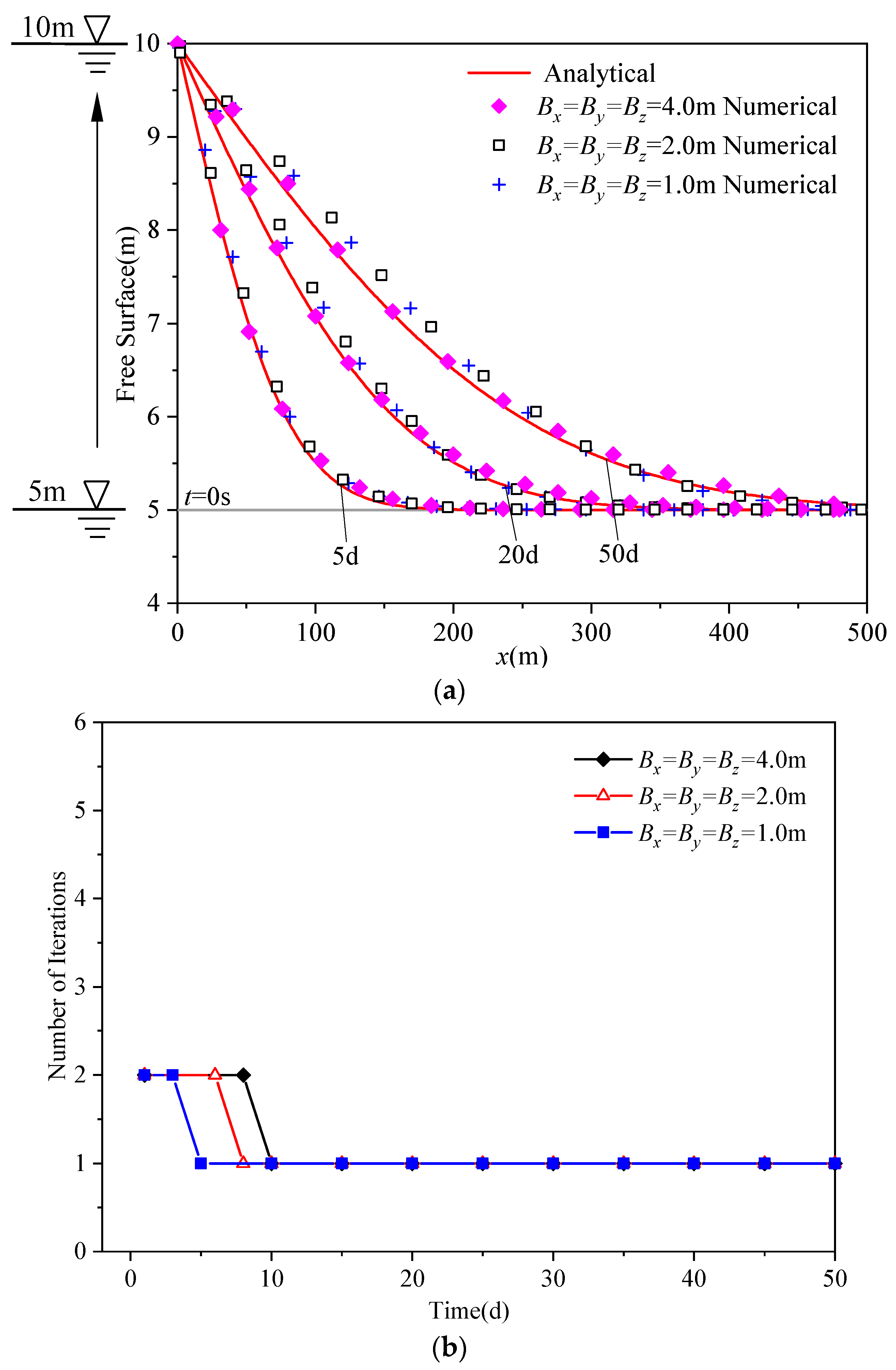
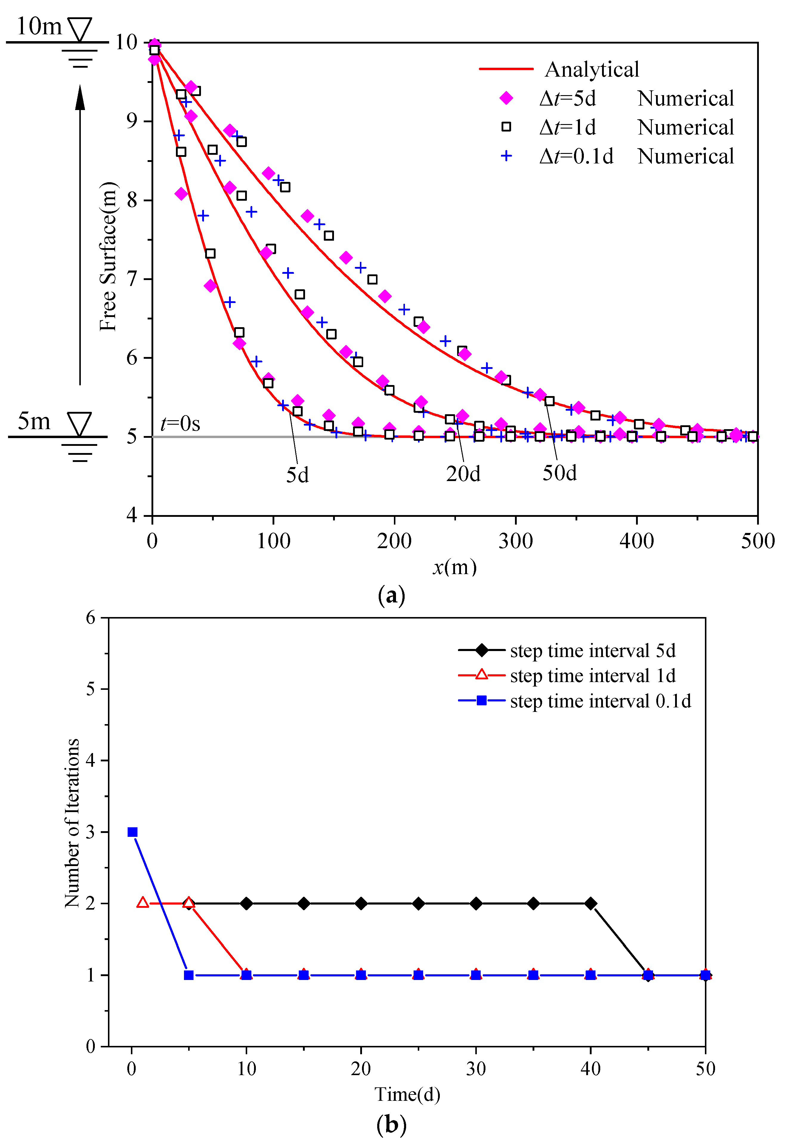
4.1. An Unconfined Aquifer

The proposed method is firstly applied to predict the evolution of transient free surfaces in a semi-infinite isotropic unconfined aquifer, as shown in Figure 3. The water level at the left boundary suddenly descends from 10 m to 5 m, this transient seepage problem through the semi-infinite unconfined aquifer is generally governed by the 1D nonlinear Boussinesq equation [30], and the analytical solution in the x direction is obtained by Zhang [30] based on the Laplace transform. The hydraulic parameters are specified as k_x = k_y = k_z = 5 m/d and μ = 0.1. To evaluate the influence of mesh size and time step on the numerical accuracy and convergence, this aquifer is meshed by a 3D orthogonal line element with different mesh sizes (B_x = B_y = B_z = 4 m, 2 m, 1 m) and simulated with various time steps ($\Delta t$ = 5 d, 1 d, 0.1 d).

Figure 4a presents the evolution of free surface locations over time from the proposed line element method, and good agreements with the analytical solutions can be commonly obtained for different mesh sizes. The variation of iteration steps over time plotted in Figure 4b shows that the numerical solutions in each timestep can be obtained with less than three iteration steps, which indicates that the convergence of the proposed line element method is fast for different mesh sizes.

Figure 5a,b shows the evolutions of free surface locations and iteration steps over time for different time steps, respectively. The mesh size is fixed as B_x = B_y = B_z = 1 m. The numerical results are almost consistent with the theoretical solutions and converge within three steps, which demonstrates that the proposed method is robust for different time steps.

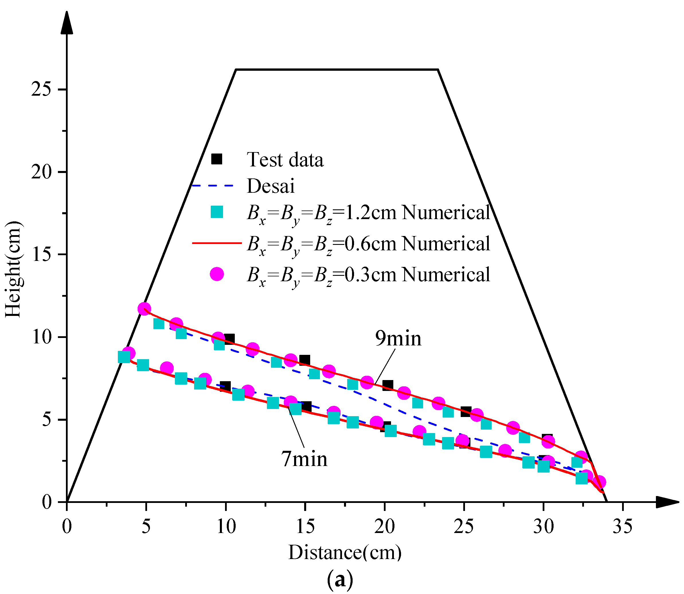
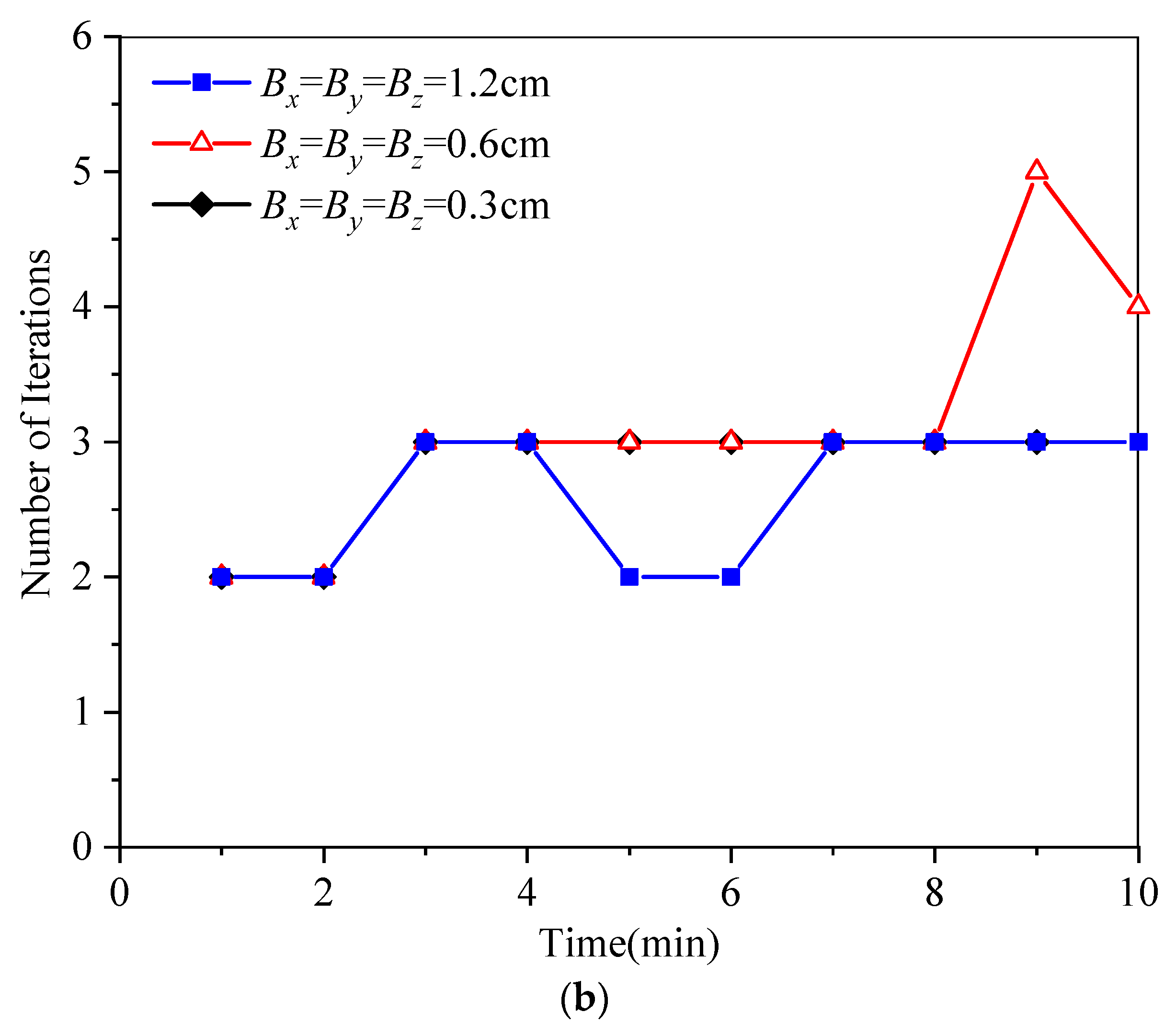
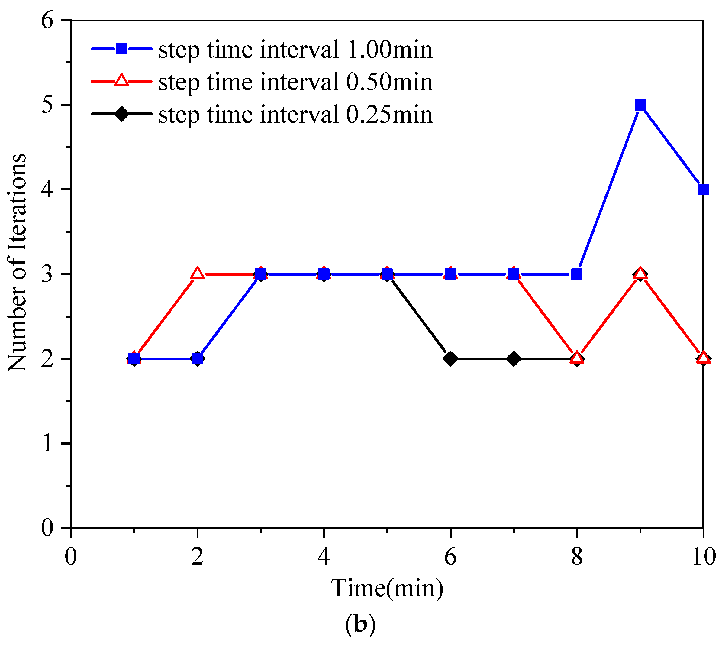
4.2. A Trapezoidal Dam

The laboratory test through a trapezoidal dam consists of the glass beads performed by Desai et al. [10] is shown in Figure 6. This isotropic dam is discretized by a 3D orthogonal network of line elements. The hydraulic parameters are given as k_x = k_y = k_z = 0.1 cm/s and μ = 0.4. The water level at the left boundary gradually increases from 0 cm to 15 cm.

Similar to the first example, the effect of mesh size and time step are shown in Figure 7 and Figure 8. For different mesh sizes, the time step is fixed as 1 min. For different time step, the mesh size is set as 0.6 cm. The model results after 7 min and 9 min agree well with the experimental data conducted by Desai et al. [10] and the computational efficiency can be well guaranteed. For comparison, the simulated data attained from Desai et al. [10] are also given, and the deviation of free surface location at 9 min is much larger than the proposed line element method.

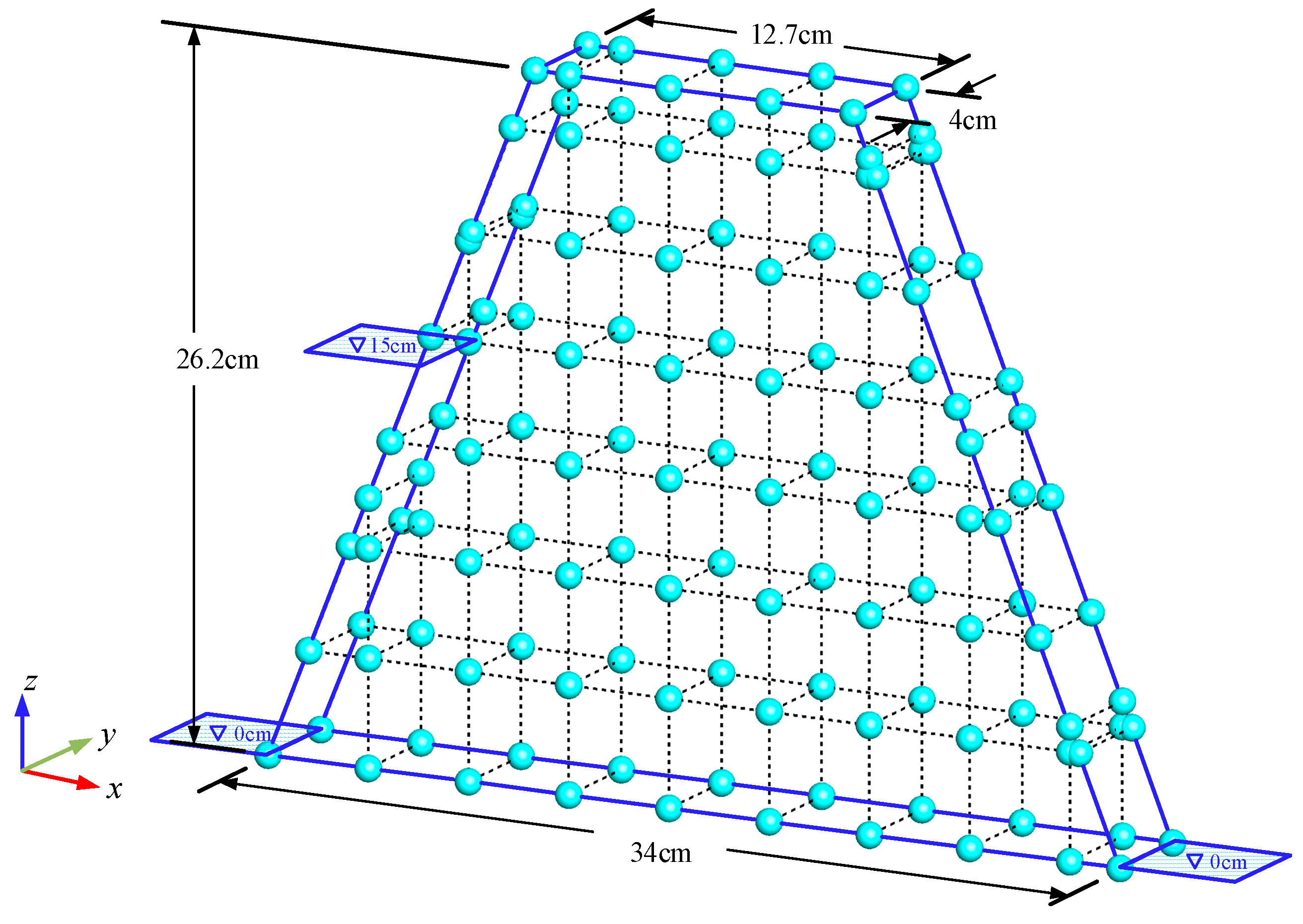
4.3. A Sand Flume

The laboratory experiment through an isotropic sand flume reported by Hu et al. [31] is illustrated in Figure 9a, which contains five rectangular drainage tunnels. The hydraulic parameters of the fine sand soil are given as k_x = k_y = k_z = 2.4 × 10⁻³ cm/s and μ = 0.05. The water level at the left boundary gradually decreases from 1.0 m to 0.2 m after 48 min, while the right water level remains at 0.2 m. During numerical analysis, the drainage tunnel is specified as a Signorini-type seepage boundary. The comparisons of free surface locations after 18 min, 30 min and 48 min between the proposed line element and observations from Hu et al. [31] are presented in Figure 9b. The calculated free surface locations are very close to the measurements and are generally achieved within 6 iteration steps.

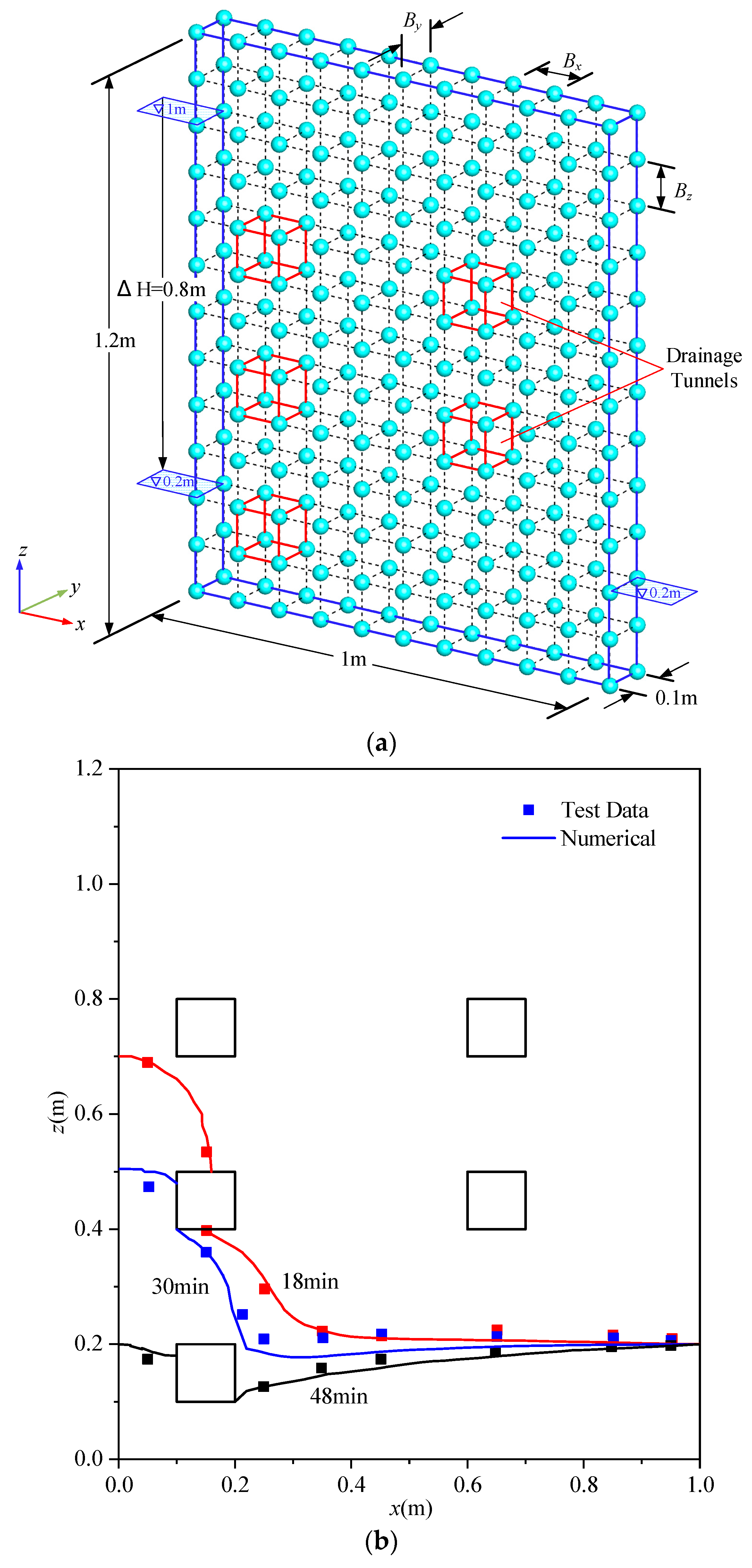
4.4. A 3D Well

Different from the previous examples with 2D condition, a 3D cylindrical well model, as shown in Figure 10a, is selected to assess the proposed method and investigate the transient free surface flow behaviors in the anisotropic porous media. The hydraulic parameters of the isotropic sand are given as k_x = k_y = k_z = 9.57 inch/min and μ = 0.3. The water level in the well decreases gradually from 48 inch to 12 inch at the initial time, while the water level of the peripheral boundary of the tank remains at 48 inch. Different from the uniform-sized element mesh in the above examples, the well model is divided into three domains meshed with non-uniformed sizes (coarse mesh 4 m, medium mesh 2 m and fine mesh 1 m) as shown in Figure 10a, in which the well with dense mesh is specified as a Signorini-type seepage boundary.

Figure 10b shows the steady free surface location after 30 min. For comparison, the experimental data from Hall [32], numerical predictions from Cooley [33] and Clement et al. [34] are also plotted. The predicted free surface is very close to the measured and other numerical results.

Besides the above isotropic case, two anisotropic cases are additionally applied to illustrate the influence of hydraulic anisotropy on the free surface variation [35,36]. The anisotropic I and II cases are specified as k_x = 10k_y = k_z = 9.57 in/min and k_x = k_y = 10k_z = 9.57 in/min, respectively. The comparisons of free surface variation with time from the isotropic and anisotropic I and II cases are shown in Figure 11. The corresponding 3D depression cones of the three cases after 5 min are presented in Figure 12.

In Figure 11b, the free surfaces almost keep horizontal around the external boundary but decline rapidly near the well with time. In Figure 11c, the variation of free surfaces are distributed evenly. Compared to the isotropic case (Figure 11a), the free surface locations at the profile x = 0 (Figure 11b) of anisotropic I turn to be much higher, while those at the profile y = 0 (Figure 11c) become much lower. This is because the decrease in k_y can lead to the increase in flow resistance and the slight hydraulic gradient in the y direction. Conversely, the flow paths in the x direction are more unimpeded in terms of seepage flow, and the hydraulic gradients are more substantial. Therefore, the corresponding 3D depression cone of anisotropic I is elliptical with different curvature at the x and y directions.

In Figure 11d, the evolution of free surfaces are not evident with time, except for the seepage points near the well. The elevations of the free surfaces are much higher than those of the isotropic case, which is in accord with the observations by Wei et al. [24]. This is because the decrease in k_z leads to the increase in flow resistance in the z direction, while the seepage flow predominantly occurs in the horizontal plane, and the hydraulic gradient becomes mild. Similar to the isotropic case, the depression cone in the anisotropic II case is also circular because of the permeability symmetry k_x = k_y but with smaller curvature. Note that this special effect cannot be characterized by the two-dimensional seepage analysis [37].

5. Conclusions

A line element method stimulated by dimension reduction is developed to model the 3D transient free surface flow in porous media, where the traditional homogeneous continuum is displaced by a 3D orthogonal network of line elements in the scale of representative elementary volume. Based on the principle of flow balance, the equivalent equations of flow velocity, continuity equation and boundary conditions are deduced to guarantee identical solution with the continuum model. Then, the finite line-element algorithm is established, in which a local 1D coordinate system is applied instead of a 3D Cartesian coordinate, and the continuous penalized Heaviside function is used to describe the whole-domain flow, including the unsaturated flow above the free surface. It is found that there is no additional calculation of hydraulic parameter and mesh reconstruction during numerical analysis. Compared to the homogeneous continuum model, the 3D transient seepage problem is simplified into a 1D system in solution space to reduce the computational cost and numerical difficulty. Through the transient free surface flow analysis in four typical examples, the numerical predictions can be achieved in few iteration steps and agree well with the analytical, experimental and other numerical results in the current literature. In addition, the hydraulic anisotropy has significant effect on the evolution of free surface locations and the shape of depression cones in spatial.

The significant advantages of the dimensional reduction based on the line element model for the transient free surface flow can be concluded as the following: (1) Easy mesh preparation. The 3D flow domain can be easily meshed into three orthogonal sets of line elements rather than the tetrahedron and hexahedron elements, and each node is connected to a maximum of six adjacent nodes (twenty-six adjacent nodes for hexahedron elements). Thus, the computational cost of mesh generation and memory storage of the nonzero elements in the matrix are greatly reduced by the dimensional reduction in the line element model. (2) Simple line integral. The line integral is much simpler than the area or volume integral through the tetrahedron and hexahedron elements, with the latter depending on the Gaussian integral points. Especially for the surface integral term ${\displaystyle {\sum }_{S_f}{\mathit{N}}^{\mathrm{T}}{u}_f\mathit{N}dxdy}$ across the jump free surface in the continuum model, the polygon shape of the free surface across the tetrahedron/hexahedron elements and the spatial plane equation based on the isoparametric element needs to be confirmed firstly. Then, the triangular subdivision is employed to calculate the contribution of flow exchange in the matrix with the specific yield. However, in the matrix F of the line element model, there is no complicated area integral and no confirmation of the surface shape; only the position of the intersection between the line element and free surface is required to calculate the value of ${\mathit{N}}^{\mathrm{T}}{u}_f\mathit{N}$. In addition, the element mesh around the free surface is fixed without updating the timestep and iteration number. The proposed method can be extended to model the 3D unsaturated seepage flow, two-phase flow and thermos problems in porous media because of the similarity between the similarity of Darcy’s law, Buckingham Law and Fourier’s law.

References

- Zhou, C.; Chen, Y.; Jiang, Q.; Lu, W. A generalized multi-field coupling approach and its application to stability and deformation control of a high slope. J. Rock Mech. Geotech. Eng. 2011, 3, 193–206. [Google Scholar] [CrossRef]
- Jiang, Q.; Qi, Z.; Wei, W.; Zhou, C. Stability assessment of a high rock slope by strength reduction finite element method. Bull. Eng. Geol. Environ. 2015, 74, 1153–1162. [Google Scholar] [CrossRef]
- Zhang, Y.; Zhang, Z.; Xue, S.; Wang, R.; Xiao, M. Stability analysis of a typical landslide mass in the Three Gorges Reservoir under varying reservoir water levels. Environ. Earth Sci. 2020, 79, 42. [Google Scholar] [CrossRef]
- Ye, Z.; Fan, X.; Zhang, J.; Sheng, J.; Chen, Y.; Fan, Q.; Qin, H. Evaluation of connectivity characteristics on the permeability of two-dimensional fracture networks using geological entropy. Water Resour. Res. 2021, 57, e2020WR029289. [Google Scholar] [CrossRef]
- Ye, Z.; Yang, J.; Xiong, F.; Huang, S.; Cheng, A. Analytical relationships between normal stress and fluid flow for single fractures based on the two-part Hooke’s model. J. Hydrol. 2022, 608, 127633. [Google Scholar] [CrossRef]
- Asghar, Z.; Ali, N.; Waqas, M.; Nazeer, M.; Khan, W.A. Locomotion of an efficient biomechanical sperm through viscoelastic medium. Biomech. Model Mechanobiol. 2020, 19, 2271–2284. [Google Scholar] [CrossRef]
- Asghar, Z.; Ali, N.; Javid, K.; Waqas, M.; Dogonchi, A.S.; Khan, W.A. Bio-inspired propulsion of micro-swimmers within a passive cervix filled with couple stress mucus. Comput. Methods Programs Biomed. 2020, 189, 105313. [Google Scholar] [CrossRef]
- Javid, K.; Waqas, M.; Asghar, Z.; Ghaffari, A. A theoretical analysis of Biorheological fluid flowing through a complex wavy convergent channel under porosity and electro-magneto-hydrodynamics Effects. Comput. Methods Programs Biomed. 2020, 191, 105413. [Google Scholar] [CrossRef]
- Neuman, S.; Witherspoon, P. Analysis of nonsteady flow with a free surface using the finite element method. Water Resour. Res. 1971, 7, 611–623. [Google Scholar] [CrossRef]
- Desai, C.S.; Lightner, J.G.; Somasundaram, S. A numerical procedure for 3D transient free surface seepage. Adv. Water Resour. 1983, 6, 175–181. [Google Scholar] [CrossRef]
- Chen, Y.; Hu, R.; Zhou, C.; Li, D.; Rong, G. A new parabolic variational inequality formulation of Signorini’s condition for non-steady seepage problems with complex seepage control systems. Int. J. Numer. Anal. Methods Geomech. 2011, 35, 1034–1058. [Google Scholar] [CrossRef]
- Rafiezadeh, K.; Ataie-Ashtiani, B. Transient free-surface seepage in 3D general anisotropic media by BEM. Eng. Anal. Bound. Elem. 2014, 46, 51–66. [Google Scholar] [CrossRef]
- Akhtar, S.; Hussain, Z.; Nadeem, S.; Najjar, I.R.; Sadoun, A.M. CFD analysis on blood flow inside a symmetric stenosed artery: Physiology of a coronary artery disease. Sci. Prog. 2023, 106, 00368504231180092. [Google Scholar] [CrossRef] [PubMed]
- Akhtar, S.; Hussain, Z.; Khan, Z.A.; Nadeem, S.; Alzabut, J. Endoscopic balloon dilation of a stenosed artery stenting via CFD tool open-foam: Physiology of angioplasty and stent placement. Chin. J. Phys. 2023, 85, 143–167. [Google Scholar] [CrossRef]
- Lin, S.; Cao, X.; Zheng, H.; Li, Y.; Li, W. An improved meshless numerical manifold method for simulating complex boundary seepage problems. Comput. Geotech. 2023, 155, 105211. [Google Scholar] [CrossRef]
- Bear, J. Dynamics of Fluids in Porous Media; Elsevier: New York, NY, USA, 1972. [Google Scholar]
- Xu, Z.H.; Ma, G.W.; Li, S.C. A graph-theoretic pipe network method for water flow simulation in a porous medium: GPNM. Int. J. Heat Fluid Flow 2014, 45, 81–97. [Google Scholar] [CrossRef]
- Afzali, S.H.; Monadjemi, P. Simulation of flow in porous media: An experimental and modeling study. J. Porous Media 2014, 17, 469–481. [Google Scholar] [CrossRef]
- Abareshi, M.; Hosseini, S.M.; Sani, A.A. Equivalent pipe network model for a coarse porous media and its application to two-dimensional analysis of flow through rockfill structures. J. Porous Media 2017, 20, 303–324. [Google Scholar] [CrossRef]
- Moosavian, N. Pipe network modelling for analysis of flow in porous media. Can. J. Civ. Eng. 2019, 46, 1151–1159. [Google Scholar] [CrossRef]
- Ye, Z.; Qin, H.; Chen, Y.; Fan, Q. An equivalent pipe network model for free surface flow in porous media. Appl. Math. Model. 2020, 87, 389–403. [Google Scholar] [CrossRef]
- Ye, Z.; Fan, Q.; Huang, S.; Cheng, A. A 1D line element model for transient free surface flow in porous media. Appl. Math. Comput. 2021, 392, 125747. [Google Scholar]
- Ren, F.; Ma, G.; Wang, Y.; Fan, L. Pipe network model for unconfined seepage analysis in fractured rock masses. Int. J. Rock Mech. Min. Sci. 2016, 88, 183–196. [Google Scholar] [CrossRef]
- Wei, W.; Jiang, Q.; Ye, Z.; Xiong, F.; Qin, H. Equivalent fracture network model for steady seepage problems with free surfaces. J. Hydrol. 2021, 603, 127156. [Google Scholar] [CrossRef]
- Chen, Y.; Zhou, C.; Zheng, H. A numerical solution to seepage problems with complex drainage systems. Comput. Geotech. 2008, 35, 383–393. [Google Scholar] [CrossRef]
- Carman, P.C. Fluid flow through granular beds. Chem. Eng. Res. Des. 1937, 15, S32–S48. [Google Scholar] [CrossRef]
- Liu, R.; Jiang, Y.; Li, B.; Yu, L. Estimating permeability of porous media based on modified Hagen-Poiseuille flow in tortuous capillaries with variable lengths. Microfluid. Nanofluid. 2016, 20, 120. [Google Scholar] [CrossRef]
- Sheng, J.; Huang, T.; Ye, Z.; Hu, B.; Liu, Y.; Fan, Q. Evaluation of van Genuchten-Mualem model on the relative permeability for unsaturated flow in aperture-based fractures. J. Hydrol. 2019, 9, 315–324. [Google Scholar] [CrossRef]
- Oden, J.T.; Kikuchi, N. Theory of variational inequalities with applications to problems of flow through porous media. Int. J. Eng. Sci. 1980, 18, 1173–1284. [Google Scholar] [CrossRef]
- Zhang, W. Calculation of Unsteady Flow of Groundwater and Evaluation of Groundwater Resources; Science Press: Beijing, China, 1983. [Google Scholar]
- Hu, R.; Chen, Y.F.; Zhou, C.B.; Liu, H.H. A numerical formulation with unified unilateral boundary condition for unsaturated flow problems in porous media. Acta Geotech. 2017, 12, 277–291. [Google Scholar] [CrossRef]
- Hall, H. An investigation of steady flow toward a gravity well. Houille Blanche 1955, 10, 8–35. [Google Scholar] [CrossRef]
- Cooley, R. Some new procedures for numerical solution of variably saturated flow problems. Water Resour. Res. 1983, 19, 1271–1285. [Google Scholar] [CrossRef]
- Clement, T.; Wise, W.; Molz, F. A physically based, two-dimensional, finitedifference algorithm for modeling variably saturated flow. J. Hydrol. 1994, 161, 71–90. [Google Scholar] [CrossRef]
- Ward, A.L.; Zhang, Z.F. Effective Hydraulic Properties Determined from Transient Unsaturated Flow in Anisotropic Soils. Vadose Zone J. 2007, 6, 913–924. [Google Scholar] [CrossRef]
- Zhang, Z.F. Relationship between Anisotropy in Soil Hydraulic Conductivity and Saturation. Vadose Zone J. 2014, 13, 1–8. [Google Scholar] [CrossRef]
- Yuan, Q.; Yin, D.; Chen, Y. A simple line-element model for three-dimensional analysis of steady free surface flow through porous media. Water 2023, 15, 1030. [Google Scholar] [CrossRef]
Disclaimer/Publisher’s Note: The statements, opinions and data contained in all publications are solely those of the individual author(s) and contributor(s) and not of MDPI and/or the editor(s). MDPI and/or the editor(s) disclaim responsibility for any injury to people or property resulting from any ideas, methods, instructions or products referred to in the content. |
© 2023 by the authors. Licensee MDPI, Basel, Switzerland. This article is an open access article distributed under the terms and conditions of the Creative Commons Attribution (CC BY) license (https://creativecommons.org/licenses/by/4.0/).
Share and Cite
Chen, Y.; Yuan, Q.; Ye, Z.; Peng, Z. A Dimension-Reduced Line Element Method for 3D Transient Free Surface Flow in Porous Media. Water 2023, 15, 3072. https://doi.org/10.3390/w15173072
Chen Y, Yuan Q, Ye Z, Peng Z. A Dimension-Reduced Line Element Method for 3D Transient Free Surface Flow in Porous Media. Water. 2023; 15(17):3072. https://doi.org/10.3390/w15173072
Chicago/Turabian StyleChen, Yuting, Qianfeng Yuan, Zuyang Ye, and Zonghuan Peng. 2023. "A Dimension-Reduced Line Element Method for 3D Transient Free Surface Flow in Porous Media" Water 15, no. 17: 3072. https://doi.org/10.3390/w15173072
APA StyleChen, Y., Yuan, Q., Ye, Z., & Peng, Z. (2023). A Dimension-Reduced Line Element Method for 3D Transient Free Surface Flow in Porous Media. Water, 15(17), 3072. https://doi.org/10.3390/w15173072