Assessing the Applicability of Mainstream Global Isoscapes for Predicting δ¹⁸O, δ²H, and d-excess in Precipitation across China

Abstract

Precipitation isoscapes have provided supporting data for numerous studies of water stable isotopes, alleviating the lack of observation data. However, the applicability of simulation data from global models to specific regional contexts remains a subject requiring further investigation, particularly concerning d-excess—an aspect often overlooked by prediction models. To bridge this gap, this study evaluates the performance of three mainstream precipitation isoscapes (OIPC3.2, RCWIP1, and RCWIP2) for the prediction of average annual δ²H, δ¹⁸O, and d-excess based on observations from the CHNIP database. The results show that while all three models can accurately reproduce δ²H and δ¹⁸O values, none are able to accurately match d-excess values. This disparity can be attributed to the absence of water-vapor source information in the models’ input variables, a key determinant influencing d-excess outcomes. Additionally, it is noteworthy that OIPC3.2 stands out as the optimal choice for δ²H and δ¹⁸O estimations, while RCWIP2 exhibits progressive enhancements over RCWIP1 in d-excess estimations. This highlights the significance of selecting highly pluralistic information variables and recognizing the impact of error propagation in such models. As a result, the advancement of isoscapes in accurately and precisely depicting precipitation isotopes, particularly d-excess, necessitates further refinement. Future avenues for improvement might involve the incorporation of water-vapor source-clustering methodologies, the selection of information-rich variables, and the autonomous construction of a dedicated d-excess simulation. This research provides valuable insights for the further refining of isoscape modeling in the future.

1. Introduction

Stable isotopes of hydrogen (²H) and oxygen (¹⁸O) are natural components of water bodies and highly sensitive to environmental changes. They provide invaluable information about the water-cycle process and are widely used in hydrology, climatology, ecology, and other fields [1,2,3,4,5,6]. Precipitation, as a pivotal component of the water cycle, serves as a primary source of terrestrial water resources. Its stable isotopic composition is essential for the characterization of hydrological processes using tracing techniques. To acquire stable isotopic data in precipitation, in situ monitoring has been conventionally employed. Prominent global and regional isotope hydro-meteorological monitoring networks like the Global Network for Isotopes in Precipitation (GNIP) [7], the United States Network of Isotopes in Precipitation (USNIP) [8,9], the Austrian Network of Isotopes in Precipitation (ANIP) [10], and the Chinese Network of Isotopes in Precipitation (CHNIP) [11] have been instrumental in providing crucial isotopic data, propelling the advancement of isotopic hydrology. Nevertheless, the endeavor is often constrained by the resource-intensive and time-consuming nature of direct precipitation isotope observations, resulting in limited spatial and temporal coverage, which falls far short of current research needs.

To address the constraints of station-based precipitation stable isotope data, considerable interest has emerged in predictive precipitation stable isotope models, commonly referred to as isoscapes. Initially, the BW model (Bowen and Wilkinson model) established regressions based on altitude and latitude [12]. Subsequently, various models have been developed, utilizing diverse climatic and geographic predictors [13,14,15,16,17]. Presently, several high-resolution isoscape products are globally available, including the Online Isotopes in Precipitation Calculator (OIPC) based on the BW model [18]; the Regionalized Cluster-Based Water Isotope Prediction (RCWIP) model, employing fuzzy clustering and regression models with multiple predictor variables [16]; and the enhanced version of RCWIP, known as RCWIP2 [19]. These isoscape products have served as invaluable supplements to observation data, mitigating data-scarcity challenges.

However, it is imperative to acknowledge that reliance solely on global isoscape models entails certain limitations. Given the diverse spatial isotopic patterns of precipitation, influenced by a myriad of climate and topographical conditions alongside complex moisture transport pathways, the unmitigated application of global isoscape products without prior verification engenders uncertainties, potentially leading to erroneous conclusions. Furthermore, while these models predominantly predict monoisotope compositions (e.g., δ²H or δ¹⁸O), the interrelationship between stable isotopes of hydrogen and oxygen in precipitation, such as their second-order variable deuterium excess (d-excess = δ²H − 8δ¹⁸O), holds critical significance in various applications, including evapotranspiration separation [20,21], groundwater recharge estimation [22], and vapor-source identification [9,23,24]. Thus, evaluating the ability of these models to accurately capture not only individual isotopes but also coupled values (d-excess) assumes paramount importance.

China’s vast geographical expanse, characterized by diverse water-vapor sources, varied climate types, and a plethora of landforms, presents an ideal testing ground for the evaluation of isoscape models. Over recent decades, these isoscape products have found widespread application in China [25,26,27]. Consequently, the objective of this study was to conduct a comprehensive assessment of the efficacy of global isoscape products—namely, OIPC, RCWIP, and RCWIP2—in predicting the δ²H, δ¹⁸O, and d-excess values of precipitation across China. Leveraging annual data from CHNIP as a verification dataset, we endeavored to address two pivotal questions: (i) to what extent do these global isoscape models accurately capture the spatial patterns of precipitation isotopes in China, and (ii) what discrepancies manifest among the three isoscape products? Through this research, we not only attempted to determine the accuracy of global isoscape products in portraying precipitation isotope information in China, but also sought to gain deeper insights into the underlying mechanisms driving the spatial variability of precipitation stable isotopes. These insights are poised to pave the way for refining isoscape modeling in future endeavors.

2. Materials and Methods

2.1. Data Sources and Processing

China is located on the west coast of the Pacific Ocean and in the east of Asia; it is affected by four types of water-vapor sources, with a diverse topography and vast land (Figure 1). From the perspective of moisture regimes, the whole country can be divided into monsoon and westerlies-dominated regions. The rainfall distribution across the monsoon regions of China is strongly seasonal in character, with a wet summer and dry winter regime as the Indian Ocean and East Asia monsoon progresses. In westerlies-dominated regions, the ocean moisture is difficult to reach, the climate is dry, and there is little rain throughout the year.

The Chinese Network of Isotopes in Precipitation (CHNIP) database was used to ensure sufficient spatial coverage and time length and, most importantly, to avoid overlap between the assessment dataset and the constructed dataset of global isoscape models. The isotopic data from the CHNIP database included 29 sites across the China continent during the 2005–2010 period (most of the stations were missing in 2008). These sites have a good representation of different geographical and climatic regions, covering the range of 21.93~47.45° N and 80.73~133.30° E, and elevations from 3.1~3688.0 m (Figure 1). The annual average temperature ranges from −0.1 to 22.4 °C and the annual average precipitation is from 51 to 1805 mm at the 29 sites (Table S1). The data of each station were precipitation amount-weighted average annual values, which could be considered to be a long-term average situation. At the same time, they were consistent with the data generated by the models in the time scale. δ²H and δ¹⁸O were expressed as δ-values, which were relative to V-SMOW (Vienna Standard Mean Ocean Water) on a normalized scale. The measurement accuracy was consistently ± 1‰ for δ²H and ± 0.3‰ for δ¹⁸O, respectively. The detailed basic information of these precipitation sampling sites is in the Supplementary Material (Table S1) [11].

Isotopes in precipitation exhibited a wide range of values among the sites (Table S1). The range of δ²H values was between −110.9‰ and −4.2‰, the δ¹⁸O values were between −15.02‰ and −1.47‰, and the d-excess values were between −6.22‰ and 13.58‰. Figure 2a,b show the spatial patterns of precipitation isotopes in CHNIP across the China continent. δ²H and δ¹⁸O in precipitation varied, a clear feature that the richer values of sites occurred in the southeast of China with the latitude increasing; the values gradually lowered from the southeast coast to Northern China (Figure 2a,b). In addition, δ²H and δ¹⁸O in precipitation were obviously depleted in the Tibetan Plateau, with a high altitude (Figure 2a,b). Comparing the spatial distribution of δ²H and δ¹⁸O, a complex pattern of the annual average d-excess distribution can be seen in Figure 2c; different values appeared randomly throughout China.

2.2. The Mainstream Precipitation Isoscape Models

The three global isoscape models considered were OIPC3.2, RCWIP1, and RCWIP2. One was OIPC3.2, released by the University of Utah [18]; the others were RCWIP1 and RCWIP2, supported by IAEA (

Table 1. Global precipitation isotope prediction models.

Models	Resolution	Established Methods	Variables	Source
OIPC3.2	5′ × 5′	BW Model	Latitude; altitude	[18]
RCWIP1	10′ × 10′	Regionalized Cluster	Geographical and climatic parameters	[16]
RCWIP2	30″ × 30″	Regionalized Cluster	Geographical and climatic parameters	[19]

).

2.2.1. OIPC3.2 Model

The OIPC3.2 model was based on observed data of GNIP. The predicted isotopes in precipitation were described as follows [12]:

$${ \mathsf{\delta }}^2\mathrm{H}/{{\mathsf{\delta }}^{18}\mathrm{O}=\mathrm{a} \left|\mathrm{LAT}\right|}^2+\mathrm{b} \left|\mathrm{LAT}\right|+\mathrm{c} \mathrm{ALT}$$

(1)

where δ²H/δ¹⁸O is the predicted value of the isotopic compositions of precipitation. LAT and ALT are the latitude in degrees and altitude in m of the stations observed, respectively, and a, b, and c are empirical parameters. Then, the residual interpolation is obtained to adjust the predictions [14]. This method regards the isotopic composition of precipitation to be mainly controlled by the temperature and regional patterns of vapor delivery are reflected in the latitude and altitude.

2.2.2. RCWIP1 Model

Compared with the OIPC model, the RCWIP model applied an approach that calculated different regression models for each climate region and merged them into a global scale through fuzzy clustering. This method can reduce the uncertainty of a global prediction. The RCWIP1 model was based on the GNIP database and some published data. The predicted isotopes in precipitation were described as follows [16]:

$${ \mathsf{\delta }}^2\mathrm{H} /{ \mathsf{\delta }}^{18}\mathrm{O}=f(\mathrm{LAT}, \mathrm{LON}, \mathrm{ALT}, \mathrm{T}, \mathrm{P}, \mathrm{VP}, \mathrm{PW})$$

(2)

where δ²H/δ¹⁸O is the predicted value of the isotopic compositions of precipitation. LON is longitude in degrees, T is air temperature in K, P is precipitation amount in mm, VP is water-vapor pressure in hPa, and PW is precipitable water in mm.

2.2.3. RCWIP2 Model

RCWIP2 added more climatic variables than RCWIP1 and predicted d-excess alone; it can be expressed as follows [19]:

$${\mathsf{\delta }}^2\mathrm{H}/ {\mathsf{\delta }}^{18}\mathrm{O}/ \mathrm{d}-\mathrm{excess}=f\left(\mathrm{LAT}, \mathrm{LON}, \mathrm{ALT}, \mathrm{T}, \mathrm{P}, \mathrm{VP}, \mathrm{PW}, \mathrm{CPN}, \mathrm{LHF}, \mathrm{NLR}, \mathrm{OLR}, \mathrm{WS}, \mathrm{wtLAT}, \mathrm{DTC}, \mathrm{LMF}\right)$$

(3)

where δ²H/δ¹⁸O/d-excess is the predicted value of the isotopic compositions of precipitation. CPN is convective precipitation intensity in mm, LHF is latent heat flux in W/m², NLR is net longwave radiation in W/m², OLR is outgoing longwave radiation in W/m², WS is wind speed in m/s, wtLAT is weighted latitude in degrees, DTC is distance to the coastline in km, and LMF is a dimensionless land-mass fraction.

The simulation data for the isotopes (δ²H, δ¹⁸O, and d-excess) at CHNIP stations were extracted from three isoscape models using ArcGIS10.7, The d-excess values for RCWIP1 and OIPC3.2 were calculated by δ²H and δ¹⁸O.

2.3. Evaluation Metric

The performance of the isoscape models was evaluated using the coefficient of determination (R²), mean error (ME), standard deviation of the error (SDE), root mean square error (RMSE), and modelling efficiency coefficient (MEC). R² is the square of Pearson’s correlation coefficient (r); it describes the linear correlation between the estimated and observed values and ranges from −1 to 1, with higher absolute values representing a better correlation. ME (accuracy error) quantifies the average error; it can be positive or negative, indicating tendencies to underestimate or overestimate. SDE (precision error) shows the random variation in the estimations after corrections for global bias. RMSE evaluates the standard deviation of the overall error in the estimation. SDE and RMSE are non-negative statistics with no upper-bound and an optimal value of 0. MEC is also known as Nash-Sutcliffe Efficiency (NSE); it quantifies the improvements made by the method using the mean of the observations as a predication. The closer MEC is to 1, the closer the estimated value is to the observed value. A negative value (MEC < 0) suggests that the model is disabled. These statistics are calculated as follows:

$$R^2=\frac{{\left[cov\left(\widehat{y_i}, y_i\right)\right]}^2}{var\left(\widehat{y_i}\right)·var\left(y_i\right)}$$

(4)

$$ME=\frac{1}{N}{\sum }_{i=1}^N\left(y_i-\widehat{y_i}\right)$$

(5)

$$SDE=\sqrt{\frac{1}{N-1}{\sum }_{i=1}^N{\left[\left(y_i-\widehat{y_i}\right)-MPE\right]}^2}$$

(6)

$$RMSE=\sqrt{\frac{{\sum }_{i=1}^N{(y_i-\widehat{y_i})}^2}{N}}$$

(7)

$$MEC=1-\frac{{{\sum }_{i=1}^N\left(y_i-\widehat{y_i}\right)}^2}{{{\sum }_{i=1}^N\left(y_i-\overline{y}\right)}^2}$$

(8)

where $y_i$, $\widehat{y_i}$, and $\overline{y}$ represent the ith observed, estimated, and mean-observed values of isotopes in precipitation, respectively. N represents the number of data instances.

In this study, a solar diagram was used together with the above statistics to provide a quick summary of the degree of method performance, allowing one to judge the relationship. On a solar diagram, the r, ME, SDE, RMSE, and MEC differences between the observed values and the estimated values are all indicated by a single point on a Cartesian coordinate system [29]. The x-axis represents the standardized ME (ME*; i.e., ME divided by the standard deviation of the observed values) and the y-axis represents the standardized SDE (SDE*; i.e., SDE divided by the standard deviation of the observed values). The distance from the origin to any point is expressed as a standardized RMSE ($RMS{E}^{*}=\sqrt{{M{E}^{*}}^2+{SD{E}^{*}}^2}$). The outer circle and the inner-circle enclosed areas denote r. The color scaling on the points represents MEC.

3. Results

3.1. Spatial Variations in Precipitation δ²H, δ¹⁸O and D-Excess

Figure 3 shows the spatial distribution of precipitation stable isotopes spanning the geographical expanse of China as predicted by the three isoscape products. The δ²H and δ¹⁸O values offered by the OIPC3.2, RCWIP, and RCWIP2 models collectively revealed akin ranges, encompassing −152.03‰ to −19.25‰, −161.00‰ to −24.10‰, and −152.57‰ to −16.82‰ for δ²H, along with −20.79‰ to −2.78‰, −19.59‰ to −4.47‰, and −20.69‰ to −3.70‰ for δ¹⁸O, correspondingly. These projected ranges inherently bore comparability with the observed values within the CHNIP dataset (Section 2.1). Remarkably, the spatial patterns of δ²H and δ¹⁸O (Figure 3a–f) derived from the three models remained consistent with the observed values (Figure 2a,b). The models effectively reproduced the δ²H and δ¹⁸O depletion trends within elevated terrains, typified by the Tibetan Plateau. Additionally, the models aptly captured the overarching spatial trend of diminishing δ²H and δ¹⁸O values from the southeastern coast towards the northern regions with ascending latitudes.

In stark contrast, the projected d-excess values presented by the three models (Figure 3g–i) notably deviated from the observed values (Figure 2c). The d-excess ranges for theOIPC3.2, RCWIP1, and RCWIP2 models were −10.76–21.23‰, −38.62–17.82‰, and 6.24–15.28‰, respectively. These projections were incongruent with the range of observed values. The RCWIP2 model portrayed a slight decrease in d-excess values from southern to northern regions, with the highest values located in the Qinghai–Tibet Plateau. Conversely, the RCWIP1 model predicted the most depleted d-excess values within the Tibetan Plateau and exhibited a declining spatial pattern from south to north, excluding this highland region. The OIPC3.2 model delineated a spatial pattern characterized by irregular fluctuations, displaying diverse values scattered across China’s expanse.

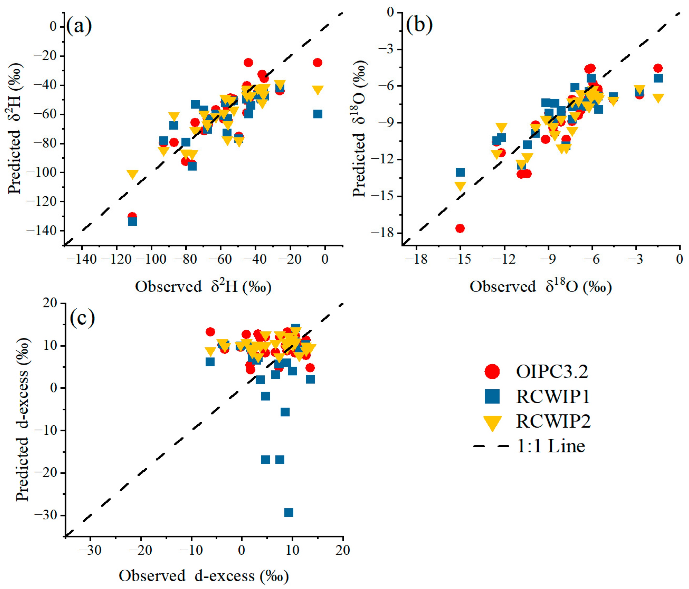
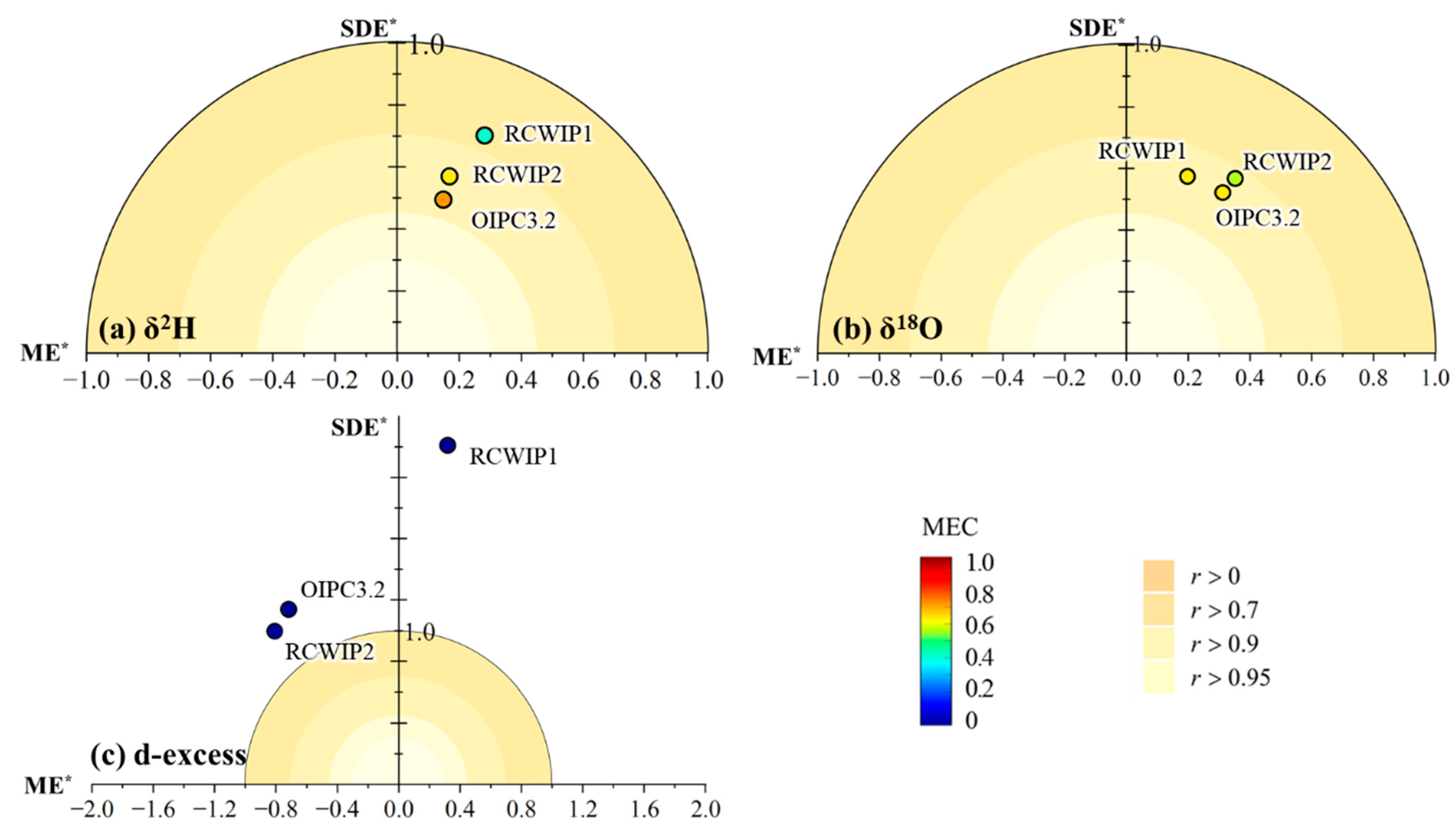
3.2. Performance Evaluation of Isoscape Models

The performance of the isoscape models in predicting stable isotopic compositions in precipitation was rigorously assessed by comparing the predicted values generated by the OIPC3.2, RCWIP1, and RCWIP2 models with their corresponding observed δ²H, δ¹⁸O, and d-excess values within the CHNIP dataset. The comparative scatter plots for these evaluations are depicted in Figure 4. In the context of δ²H and δ¹⁸O in precipitation, the datapoints for each model in the figures closely aligned with the 1:1 reference line, with only a limited number of sites displaying significant deviations (Figure 4a,b). In stark contrast, the predicted d-excess values across the three isoscape models exhibited a notable departure from the 1:1 line, with the majority of datapoints deviating significantly (Figure 4c).

The metrics presented in

Table 2. Performance statistics of precipitation stable isotopes using the OIPC3.2, RCWIP1, and RCWIP2 models.

Models	Objects	R2	ME	SDE	RMSE	MEC
OIPC3.2	δ2H	0.78	3.21	10.63	11.11	0.73
	δ18O	0.75	0.87	1.45	1.69	0.63
	D-excess	0.00	−3.74	5.94	7.02	−0.81
RCWIP1	δ2H	0.53	6.07	15.09	16.27	0.43
	δ18O	0.69	0.55	1.60	1.69	0.63
	D-excess	0.01	1.66	11.53	11.65	−3.99
RCWIP2	δ2H	0.68	3.64	12.25	12.78	0.65
	δ18O	0.69	0.98	1.58	1.86	0.55
	D-excess	0.02	−4.22	5.20	6.69	−0.65

Notes: R²: coefficient of determination; ME: mean error; SDE: standard deviation of the error; RMSE: root mean squared error; MEC: modelling efficiency coefficient.

further substantiate these observations, providing statistical performance data for precipitation stable isotopes as predicted by the OIPC3.1, RCWIP1, and RCWIP2 isoscape models. Cumulatively, the models demonstrated commendable performance, as evidenced by high R² and MEC values and low |ME|, SDE, and RMSE metrics for δ²H and δ¹⁸O. However, predictions for d-excess revealed a disparate pattern. Here, the models yielded high values for |ME|, SDE, RMSE, near zero R² values, and negative MEC scores. These trends unequivocally demonstrated the three models’ capacity to accurately replicate δ²H and δ¹⁸O values whilst concurrently underscoring their limitations in predicting d-excess.

3.3. Comparative Analysis of Three Isoscape Models

In Figure 5, a solar diagram is utilized to expediently assess the relationships between the OIPC3.2, RCWIP1, and RCWIP2 models in comparison with the observed values. For the δ²H solar diagram (Figure 5a), the x-axis ME* values distinctly highlighted a positive bias across all three models, with RCWIP1 exhibiting the highest bias, followed by RCWIP2 and OIPC3.2. The corresponding SDE* and RMSE* values echoed the ME* trend. Notably, the OIPC3.2 model displayed the highest MEC value (0.73) and r value (0.88). Subsequently, RCWIP2 showed slightly lower, yet commendable MEC (0.65) and r (0.82) values, while RCWIP1 demonstrated the lowest MEC (0.43) and r (0.73) values. Consequently, among the three models, OIPC3.2 emerged as the premier predictor for δ²H, trailed by RCWIP2 and RCWIP1.

Turning to the δ¹⁸O solar diagram (Figure 5b), the OIPC3.2 model showed superior performance, characterized by a lower RMSE* value (0.61) as well as better MEC (0.63) and r (0.87) values compared with RCWIP1 and RCWIP2. Although RCWIP1 slightly outperformed OIPC3.2 in terms of accuracy (lower ME*), its precision was comparatively diminished (higher SDE*). RCWIP2 demonstrated a larger RMSE* value (0.67) and a reduced MEC (0.55) compared with OIPC3.2 and RCWIP1. Importantly, while differences existed among the three models’ predictions of δ¹⁸O, the overall disparities were relatively minimal. Shifting focus to the δ¹⁸O solar diagram (Figure 5b), the OIPC3.2 model exhibited superior performance, evidenced by a lower RMSE* value (0.61) coupled with improved MEC (0.63) and r (0.87) values compared with RCWIP1 and RCWIP2. Although RCWIP1 marginally surpassed OIPC3.2 in terms of accuracy (lower ME*), its precision was relatively compromised (higher SDE*). Meanwhile, RCWIP2 yielded a larger RMSE* value (0.67) and decreased MEC (0.55) in contrast to OIPC3.2 and RCWIP1. Although differences existed in the δ¹⁸O predictions among the models, the overall discrepancies remained modest.

In the d-excess solar diagram (Figure 5c), all three models deviated beyond the outermost circle at a RMSE* of 1, indicating that employing these models did not yield improved predictions over utilizing the observed mean value as a d-excess predictor in precipitation. Both MEC and r values underscored the models’ unsuitability for d-excess prediction. Notably, significant distinctions were evident among the three models. RCWIP1 exhibited a smaller ME* compared with the other models, but its SDE* was considerably higher, signifying reduced precision. In contrast, RCWIP2 and OIPC3.2 showcased remarkable precision enhancement without an equivalent boost in accuracy.

4. Discussion

4.1. Why Is the Performance of Isoscape Models Better for δ²H (δ¹⁸O) than for d-excess?

The outcomes demonstrated that the annual estimates of δ²H and δ¹⁸O produced by the three isoscape models (Figure 3) effectively replicated the observed values (Figure 2), with all three models achieving favorable scores according to the statistical evaluation index (Table 2). These findings align with prior research evaluating the performance of OIPC or RCWIP models within specific regions [25,26,30]. As such, a general consensus emerges from these studies, underscoring the isoscape models’ capability to characterize and predict annual individual isotopes (δ²H or δ¹⁸O). Both δ²H and δ¹⁸O offer insights into the relative content of ²H and ¹⁸O within a water body, undergoing changes due to various physical and chemical processes during the water cycle [31,32,33,34]. Consequently, these isotopes tend to exhibit strong correlations with environmental variables such as latitude, altitude, proximity to coastlines, air temperature, and precipitation volume, a phenomenon well-documented both in China and globally [11,31,35,36]. The isoscape models under scrutiny here predicted stable isotopes in precipitation based on environmental variables [12,16,19], which explains their successful performance in δ²H and δ¹⁸O estimations.

Furthermore, it is important to note that the three models manifested negligible discrepancies in annual single-isotope predictions (δ²H and δ¹⁸O), as evidenced by the standard deviations of RMSE being 2.15‰ and 0.08‰, respectively (Table 2). Variations in model input data, structures, and parameters have the potential to impact predicted outcomes [37]. Given the reliance of the three models on environmental variables [12,16,19], the marginal disparities in their estimates likely resulted from divergences in input data and parameter choices. Moreover, the disparity in estimates among the models pales in comparison with the observed value variability across China (Figure 2), a similarity also noted in previous investigations of single stable isotope estimations within China [27]. As such, it is reasonable to consider the three models as viable options when observed data of δ²H and δ¹⁸O are lacking.

However, despite the favorable performance exhibited in the estimation of individual isotopes (δ²H and δ¹⁸O), the computed d-excess values significantly deviated from the observed d-excess values in China (Table 2; Figure 4). Adequately capturing the d-excess trend proves to be a challenging endeavor for isoscape models as most evaluation studies have primarily focused on the performance of δ²H and δ¹⁸O estimations [25,26,30], with only a handful touching on this phenomenon [19,38]. The inability of isoscape models to accurately predict d-excess is likely due to the models using environmental variables containing little or no water-vapor source information. D-excess, expressed as d-excess = δ²H − 8δ¹⁸O, serves as a measure of kinetic isotopic fractionation during the water cycle [31,39]. Consequently, two main processes of changing d-excess can be summarized: variations in water-vapor sources and the evaporation effect of descending raindrops. Both are closely tied to the meteorological conditions of the water-vapor source region [31,33,39,40] and the local environment, respectively [41,42,43]. As the three models hinge on environmental variables [12,16,19], they inherently represent only one of these processes. Moreover, sub-cloud evaporation, a process captured by the models that influences d-excess values, usually plays a key role in small precipitation events, but is not significant at monthly or annual scales [44,45]. Consequently, these isoscape models describe only a fraction of the variations, rendering them inadequate for d-excess estimations.

4.2. What Are the Differences between the Three Models?

While all three models exhibited competence in predicting average annual single isotopes (δ²H and δ¹⁸O), the evaluation outcomes highlight a slight advantage for OIPC3.2. This model not only boasted the lowest RMSE* values, but also attained MEC and r values closest to 1 in average annual δ²H and δ¹⁸O estimates (Table 2 and Figure 5).

OIPC3.2 relies on a regression approach built upon spatial variables, including latitude and altitude [12]. In contrast, RCWIP1 [16] and RCWIP2 [19] incorporate an extended set of climatic and spatial variables, encompassing parameters such as air temperature, precipitation amount, water-vapor pressure, convective precipitation intensity, and distance to coastlines. Surprisingly, the augmentation of variables in RCWIP models does not yield a proportional enhancement in interpretation for average annual δ²H and δ¹⁸O, potentially attributed to the redundancy of these variables, leading to over-interpretation. This redundancy arises from the fact that several climatic variables, including temperature, precipitation, and relative humidity, already exert strong spatial (latitudinal and altitudinal) controls [17,46]. Consequently, OIPC3.2’s utilization of highly pluralistic information variables affords it a marginal lead in average annual δ²H and δ¹⁸O estimates while maintaining a simpler model structure.

In the realm of d-excess predictions, it was evident that RCWIP2 surpassed RCWIP1 and even outperformed OIPC3.2, although the current mainstream isoscape models largely faltered in d-excess estimates (Figure 5). In comparison with OIPC3.2 [18], the RCWIP models incorporate a fuzzy clustering methodology based on climatic zones [16,19]. However, this approach failed to notably reduce ME* relative to OIPC3.2 (Table 2), signifying the limited capacity of climate zoning to enhance d-excess estimation accuracy. Notably, RCWIP2, as an upgraded iteration of RCWIP1, independently constructed a d-excess model, resulting in a considerable reduction in SDE* (Figure 5c and Table 2). This reduction may be attributed to mitigated cumulative error propagation stemming from the incorporation of predicted δ²H and δ¹⁸O values influenced by various climatic and spatial variables. Many studies have also indicated that the error propagation will cause a larger bias in hydrological model simulations [47,48].

4.3. The Direction for Isoscape Model Improvements

Our evaluation results underscore the potential for further enhancements in isoscape models, particularly concerning d-excess. The analysis above suggests that instead of introducing a surplus of environmental variables, a more effective avenue for refinement involves considering new explanatory variables that encompass water-vapor source information. The addition of more variables may not yield a significant improvement in model performance, as seen in our findings.

However, addressing the effects of water-vapor sources poses a notable challenge, necessitating the exploration of alternative methodologies. One promising approach could involve water-vapor source clustering, which has the potential to refine existing climate zoning methods employed in models like RCWIP. A precedent for this method exists in a prior study that employed water-vapor source clustering to mitigate the influence of diverse vapor sources on isotopic estimates in precipitation [49]. The viability of this technique was demonstrated in Australia, where an isoscape model used clusters of both climate and water-vapor sources rather than solely relying on climate clusters to predict d-excess in precipitation [30]. Consequently, future isoscape models could potentially incorporate a water-vapor source and fuzzy clustering method to account for the combined effects of multiple water-vapor sources. Furthermore, the independent construction of RCWIP2 for d-excess resulted in a significant decrease in SDE* (Figure 5c), which greatly improved the simulation accuracy. To reduce the effect of error propagation, it is feasible to separately build a d-excess model. This departure from relying only on the conventional expression of d-excess offers a tangible pathway to elevate the reliability of modeled outcomes.

5. Conclusions

In this study, we evaluated three models (OIPC3.2, RCWIP1, and RCWIP2) for the estimation of average annual δ¹⁸O, δ²H, and d-excess based on observations from the CHNIP database, and drew the following conclusions: (i) The evaluation results demonstrated that the three models accurately reproduced δ²H and δ¹⁸O values; however, they yielded unmatched results for d-excess. This discrepancy primarily stemmed from the absence of water-vapor source information within the variables inputted into the models. While δ²H and δ¹⁸O are mainly controlled by environmental factors, d-excess is notably more influenced by the source of the water vapor. (ii) Among the three models, OIPC3.2 outperformed the other models in estimating δ²H and δ¹⁸O. Despite all three models proving inefficient for d-excess, an incremental improvement was noticed in RCWIP2 versus RCWIP1. This highlights the significance of selecting appropriate regression variables and recognizing the impact of error propagation. Moving forward, the use of water-vapor source-clustering methodology, selecting variables containing more extensive information, and constructing a separate d-excess model might provide future improvement avenues to advance the accuracy and reliability of isoscape model predictions.

References

1. Marx, C.; Tetzlaff, D.; Hinkelmann, R.; Soulsby, C. Seasonal Variations in Soil-Plant Interactions in Contrasting Urban Green Spaces: Insights from Water Stable Isotopes. J. Hydrol. 2022, 612, 127998. [Google Scholar] [CrossRef]
2. Lu, Y.; Wen, M.; Li, P.; Liang, J.; Wei, H.; Li, M. An Improved Craig-Gordon Isotopic Model: Accounting for Transpiration Effects on the Isotopic Composition of Residual Water during Evapotranspiration. Agronomy 2023, 13, 1531. [Google Scholar] [CrossRef]
3. Boosalik, Z.; Jafari, H.; Clark, I.D.; Bagheri, R. Chemo-Isotopic Tracing of the Groundwater Salinity in Arid Regions: An Example of Shahrood Aquifer (Iran). J. Geochem. Explor. 2022, 239, 107029. [Google Scholar] [CrossRef]
4. Brkić, Ž.; Briški, M.; Marković, T. Use of Hydrochemistry and Isotopes for Improving the Knowledge of Groundwater Flow in a Semiconfined Aquifer System of the Eastern Slavonia (Croatia). CATENA 2016, 142, 153–165. [Google Scholar] [CrossRef]
5. Sprenger, M.; Stumpp, C.; Weiler, M.; Aeschbach, W.; Allen, S.T.; Benettin, P.; Dubbert, M.; Hartmann, A.; Hrachowitz, M.; Kirchner, J.W.; et al. The Demographics of Water: A Review of Water Ages in the Critical Zone. Rev. Geophys. 2019, 57, 800–834. [Google Scholar] [CrossRef]
6. Lu, Y.; Li, H.; Si, B.; Li, M. Chloride Tracer of the Loess Unsaturated Zone under Sub-Humid Region: A Potential Proxy Recording High-Resolution Hydroclimate. Sci. Total Environ. 2020, 700, 134465. [Google Scholar] [CrossRef] [PubMed]
7. IAEA/WMO. Global Network of Isotopes in Precipitation. In The GNIP Database; IAEA: Vienna, Austria, 2021. [Google Scholar]
8. Welker, J.M. Isotopic (Δ18O) Characteristics of Weekly Precipitation Collected across the USA: An Initial Analysis with Application to Water Source Studies. Hydrol. Process 2000, 14, 1449–1464. [Google Scholar] [CrossRef]
9. Welker, J.M. ENSO Effects on Δ18O, Δ2H and d-Excess Values in Precipitation across the U.S. Using a High-Density, Long-Term Network (USNIP). Rapid Commun. Mass. Spectrom. 2012, 26, 1893–1898. [Google Scholar] [CrossRef]
10. Allen, S.T.; Kirchner, J.W.; Goldsmith, G.R. Predicting Spatial Patterns in Precipitation Isotope (Δ2H and Δ18O) Seasonality Using Sinusoidal Isoscapes. Geophys. Res. Lett. 2018, 45, 4859–4868. [Google Scholar] [CrossRef]
11. Liu, J.; Song, X.; Yuan, G.; Sun, X.; Yang, L. Stable Isotopic Compositions of Precipitation in China. Tellus B Chem. Phys. Meteorol. 2014, 66, 22567. [Google Scholar] [CrossRef]
12. Bowen, G.J.; Wilkinson, B. Spatial Distribution of Delta O-18 in Meteoric Precipitation. Geology 2002, 30, 315–318. [Google Scholar] [CrossRef]
13. Erdélyi, D.; Hatvani, I.G.; Jeon, H.; Jones, M.; Tyler, J.; Kern, Z. Predicting Spatial Distribution of Stable Isotopes in Precipitation by Classical Geostatistical- and Machine Learning Methods. J. Hydrol. 2023, 617, 129129. [Google Scholar] [CrossRef]
14. Bowen, G.J.; Revenaugh, J. Interpolating the Isotopic Composition of Modern Meteoric Precipitation. Water Resour. Res. 2003, 39, 1299. [Google Scholar] [CrossRef]
15. Lykoudis, S.P.; Argiriou, A.A. Gridded Data Set of the Stable Isotopic Composition of Precipitation over the Eastern and Central Mediterranean. J. Geophys. Res. Atmos. 2007, 112. [Google Scholar] [CrossRef]
16. Terzer, S.; Wassenaar, L.I.; Araguás-Araguás, L.J.; Aggarwal, P.K. Global Isoscapes for Δ18O and Δ2H in Precipitation: Improved Prediction Using Regionalized Climatic Regression Models. Hydrol. Earth Syst. Sci. 2013, 17, 4713–4728. [Google Scholar] [CrossRef]
17. Valdivielso, S.; Hassanzadeh, A.; Vázquez-Suñé, E.; Custodio, E.; Criollo, R. Spatial Distribution of Meteorological Factors Controlling Stable Isotopes in Precipitation in Northern Chile. J. Hydrol. 2022, 605, 127380. [Google Scholar] [CrossRef]
18. Bowen, G.J.; Wassenaar, L.I.; Hobson, K.A. Global Application of Stable Hydrogen and Oxygen Isotopes to Wildlife Forensics. Oecologia 2005, 143, 337–348. [Google Scholar] [CrossRef]
19. Terzer-Wassmuth, S.; Wassenaar, L.I.; Welker, J.M.; Araguás-Araguás, L.J. Improved High-Resolution Global and Regionalized Isoscapes of Δ18O, Δ2H and d-Excess in Precipitation. Hydrol. Process. 2021, 35, e14254. [Google Scholar] [CrossRef]
20. Zhang, F.; Huang, T.; Man, W.; Hu, H.; Long, Y.; Li, Z.; Pang, Z. Contribution of Recycled Moisture to Precipitation: A Modified D-Excess-Based Model. Geophys. Res. Lett. 2021, 48, e2021GL095909. [Google Scholar] [CrossRef]
21. Froehlich, K.; Kralik, M.; Papesch, W.; Rank, D.; Scheifinger, H.; Stichler, W. Deuterium Excess in Precipitation of Alpine Regions—Moisture Recycling. Isot. Environ. Health Stud. 2008, 44, 61–70. [Google Scholar] [CrossRef]
22. Krishan, G.; Prasad, G.; Anjali; Kumar, C.P.; Patidar, N.; Yadav, B.K.; Kansal, M.L.; Singh, S.; Sharma, L.M.; Bradley, A.; et al. Identifying the Seasonal Variability in Source of Groundwater Salinization Using Deuterium Excess- a Case Study from Mewat, Haryana, India. J. Hydrol. Reg. Stud. 2020, 31, 100724. [Google Scholar] [CrossRef]
23. Landais, A.; Risi, C.; Bony, S.; Vimeux, F.; Descroix, L.; Falourd, S.; Bouygues, A. Combined Measurements of 17Oexcess and D-Excess in African Monsoon Precipitation: Implications for Evaluating Convective Parameterizations. Earth Planet. Sci. Lett. 2010, 298, 104–112. [Google Scholar] [CrossRef]
24. Vallet-Coulomb, C.; Gasse, F.; Sonzogni, C. Seasonal Evolution of the Isotopic Composition of Atmospheric Water Vapour above a Tropical Lake: Deuterium Excess and Implication for Water Recycling. Geochim. Cosmochim. Acta 2008, 72, 4661–4674. [Google Scholar] [CrossRef]
25. Shi, X.; Risi, C.; Pu, T.; Lacour, J.-L.; Kong, Y.; Wang, K.; He, Y.; Xia, D. Variability of Isotope Composition of Precipitation in the Southeastern Tibetan Plateau from the Synoptic to Seasonal Time Scale. J. Geophys. Res. Atmos. 2020, 125, e2019JD031751. [Google Scholar] [CrossRef]
26. Chen, F.; Zhang, M.; Wang, S.; Qiu, X.; Du, M. Environmental Controls on Stable Isotopes of Precipitation in Lanzhou, China: An Enhanced Network at City Scale. Sci. Total Environ. 2017, 609, 1013–1022. [Google Scholar] [CrossRef]
27. Wang, S.; Zhang, M.; Bowen, G.J.; Liu, X.; Du, M.; Chen, F.; Qiu, X.; Wang, L.; Che, Y.; Zhao, G. Water Source Signatures in the Spatial and Seasonal Isotope Variation of Chinese Tap Waters. Water Resour. Res. 2018, 54, 9131–9143. [Google Scholar] [CrossRef]
28. Araguás-Araguás, L.; Froehlich, K.; Rozanski, K. Stable Isotope Composition of Precipitation over Southeast Asia. J. Geophys. Res. Atmos. 1998, 103, 28721–28742. [Google Scholar] [CrossRef]
29. Wadoux, A.M.J.C.; Walvoort, D.J.J.; Brus, D.J. An Integrated Approach for the Evaluation of Quantitative Soil Maps through Taylor and Solar Diagrams. Geoderma 2022, 405, 115332. [Google Scholar] [CrossRef]
30. Hollins, S.E.; Hughes, C.E.; Crawford, J.; Cendon, D.I.; Meredith, K.T. Rainfall Isotope Variations over the Australian Continent—Implications for Hydrology and Isoscape Applications. Sci. Total Environ. 2018, 645, 630–645. [Google Scholar] [CrossRef]
31. Dansgaard, W. Stable Isotopes in Precipitation. Tellus 1964, 16, 436–468. [Google Scholar] [CrossRef]
32. Bedaso, Z.; Wu, S.Y. Daily Precipitation Isotope Variation in Midwestern United States: Implication for Hydroclimate and Moisture Source. Sci. Total Environ. 2020, 713, 136631. [Google Scholar] [CrossRef] [PubMed]
33. Wu, S.-Y.; Bedaso, Z. Quantifying the Effect of Moisture Source and Transport on the Precipitation Isotopic Variations in Northwest Ethiopian Highland. J. Hydrol. 2022, 605, 127322. [Google Scholar] [CrossRef]
34. Islam, M.R.; Gao, J.; Ahmed, N.; Karim, M.M.; Bhuiyan, A.Q.; Ahsan, A.; Ahmed, S. Controls on Spatiotemporal Variations of Stable Isotopes in Precipitation across Bangladesh. Atmos. Res. 2021, 247, 105224. [Google Scholar] [CrossRef]
35. Zhang, M.; Wang, S. A Review of Precipitation Isotope Studies in China: Basic Pattern and Hydrological Process. J. Geogr. Sci. 2016, 26, 921–938. [Google Scholar] [CrossRef]
36. Natali, S.; Baneschi, I.; Doveri, M.; Giannecchini, R.; Selmo, E.; Zanchetta, G. Meteorological and Geographical Control on Stable Isotopic Signature of Precipitation in a Western Mediterranean Area (Tuscany, Italy): Disentangling a Complex Signal. J. Hydrol. 2021, 603, 126944. [Google Scholar] [CrossRef]
37. Bai, P. Comparison of Remote Sensing Evapotranspiration Models: Consistency, Merits, and Pitfalls. J. Hydrol. 2023, 617, 128856. [Google Scholar] [CrossRef]
38. Shi, Y.; Wang, S.; Zhang, M.; Li, Y.; Song, Y. Applicability on the OIPC and RCWIP stable hydrogen and oxygen isotope data in precipitation across the Tianshan Mountains, Xinjiang. J. Glaciol. Geocryol. 2020, 42, 974–985. [Google Scholar] [CrossRef]
39. Xia, Z.; Welker, J.M.; Winnick, M.J. The Seasonality of Deuterium Excess in Non-Polar Precipitation. Glob. Biogeochem. Cycles 2022, 36, e2021GB007245. [Google Scholar] [CrossRef]
40. Merlivat, L.; Jouzel, J. Global Climatic Interpretation of the Deuterium-Oxygen 18 Relationship for Precipitation. J. Geophys. Res. Ocean. 1979, 84, 5029–5033. [Google Scholar] [CrossRef]
41. Dee, S.; Bailey, A.; Conroy, J.L.; Atwood, A.; Stevenson, S.; Nusbaumer, J.; Noone, D. Water Isotopes, Climate Variability, and the Hydrological Cycle: Recent Advances and New Frontiers. Environ. Res. Clim. 2023, 2, 022002. [Google Scholar] [CrossRef]
42. Salamalikis, V.; Argiriou, A.A.; Dotsika, E. Isotopic Modeling of the Sub-Cloud Evaporation Effect in Precipitation. Sci. Total Environ. 2016, 544, 1059–1072. [Google Scholar] [CrossRef] [PubMed]
43. Crawford, J.; Hollins, S.E.; Meredith, K.T.; Hughes, C.E. Precipitation Stable Isotope Variability and Subcloud Evaporation Processes in a Semi-Arid Region. Hydrol. Process. 2017, 31, 20–34. [Google Scholar] [CrossRef]
44. Wang, L.; Wang, S.; Zhang, M.; Duan, L.; Xia, Y. An Hourly-Scale Assessment of Sub-Cloud Evaporation Effect on Precipitation Isotopes in a Rainshadow Oasis of Northwest China. Atmos. Res. 2022, 274, 106202. [Google Scholar] [CrossRef]
45. Wang, S.; Zhang, M.; Hughes, C.E.; Crawford, J.; Wang, G.; Chen, F.; Du, M.; Qiu, X.; Zhou, S. Meteoric Water Lines in Arid Central Asia Using Event-Based and Monthly Data. J. Hydrol. 2018, 562, 435–445. [Google Scholar] [CrossRef]
46. Houston, J. Variability of Precipitation in the Atacama Desert: Its Causes and Hydrological Impact. Int. J. Clim. 2006, 26, 2181–2198. [Google Scholar] [CrossRef]
47. Zhu, D.; Peng, D.Z.; Cluckie, I.D. Statistical Analysis of Error Propagation from Radar Rainfall to Hydrological Models. Hydrol. Earth Syst. Sci. 2013, 17, 1445–1453. [Google Scholar] [CrossRef]
48. Worako, A.W.; Haile, A.T.; Rientjes, T.; Woldesenbet, T.A. Error Propagation of Climate Model Rainfall to Streamflow Simulation in the Gidabo Sub-Basin, Ethiopian Rift Valley Lakes Basin. Hydrol. Sci. J. 2022, 67, 1185–1198. [Google Scholar] [CrossRef]
49. Liu, Z.; Tian, L.; Chai, X.; Yao, T. A Model-Based Determination of Spatial Variation of Precipitation Δ18O over China. Chem. Geol. 2008, 249, 203–212. [Google Scholar] [CrossRef]
Figure 1. Locations of precipitation sampling sites and atmospheric circulation (colored lines represent the maximum extent of major air masses controlling weather patterns of China according to Araguás [28]).
Water 15 03181 g001
Figure 2. The spatial pattern of stable isotopes in precipitation based on observations of CHNIP: (a) δ2H; (b) δ18O; (c) d-excess.
Water 15 03181 g002
Figure 3. The spatial pattern of stable isotopes in precipitation across China obtained by OIPC3.2 ((a) δ2H; (d) δ18O; (g) d-excess), RCWIP1 ((b) δ2H; (e) δ18O; (h) d-excess) and RCWIP2 ((c) δ2H; (f) δ18O; (i) d-excess).
Water 15 03181 g003
Figure 4. Scatterplots of the observed and predicted δ2H (a), δ18O (b), and d-excess (c) at each site of CHNIP.
Water 15 03181 g004
Figure 5. Solar diagram of isoscape models for the prediction of δ2H, δ18O, and d-excess compared with the reference point (precipitation isotopes’ observations) at coordinates (0, 0). The outer circle and the inner-circle enclosed areas identify where r is greater than 0, 0.7, 0.9, and 0.95. The color scaling on the points represents the modelling efficiency coefficient (MEC) between the observations and predictions. The x-axis represents the standardized ME (ME*; i.e., ME divided by the standard deviation of the observed values) and the y-axis represents the standardized SDE (SDE*; i.e., SDE divided by the standard deviation of the observed values).
Water 15 03181 g005