Article

Geophysical Constraints to Reconstructing the Geometry of a Shallow Groundwater Body in Caronia (Sicily)

1
Department of Earth and Marine Sciences (DISTEM), Università degli Studi di Palermo, 90123 Palermo, Italy
2
Istituto Nazionale di Geofisica e Vulcanologia, Sezione di Palermo, 90146 Palermo, Italy
*
Author to whom correspondence should be addressed.
Water 2023, 15(18), 3206; https://doi.org/10.3390/w15183206
Submission received: 31 July 2023 / Revised: 24 August 2023 / Accepted: 4 September 2023 / Published: 8 September 2023
(This article belongs to the Special Issue Application of Geophysical Methods for Hydrogeology)

Abstract

:
The characterization of a groundwater body involves the construction of a conceptual model that constitutes the base knowledge for monitoring programs, hydrogeological risk assessment, and correct management of water resources. In particular, a detailed geological and geophysical approach was applied to define the alluvial Caronia Groundwater Body (CGWB) and to reconstruct a hydrogeological flow model. The analysis of the CGWB, located in north-eastern Sicily, was initially approached through a reanalysis of previous stratigraphic (boreholes) and geophysical (vertical electrical soundings and seismic refraction profiles) data, subsequently integrated by new seismic acquisitions, such as Multichannel Analysis of Surface Waves (MASW) and horizontal-to-vertical seismic ratio (HVSR). The analysis and reinterpretation of geoelectrical data allowed the construction of a preliminary 3D resistivity model. This initial modeling was subsequently integrated by a geophysical data campaign in order to define the depth of the bottom of the shallow CGWB and the thickness of alluvial deposits. Finally, a preliminary mathematical model flow was generated in order to reconstruct the dynamics of underground water. The results show that integration of multidisciplinary data represent an indispensable tool for the characterization of complex physical systems.

1. Introduction

The definition of the hydrogeological features of a specific territory represents an important topic because the protection and management of water resources are matters of public interest, and there is growing concern about underground water resources quality and quantity [1,2,3]. Until a few decades ago, the study of hydrogeological structures was carried out mainly using stratigraphic data derived from field geology, drilling, and logging [4,5] as well as from aquifer test methods [6,7]. Many authors instead used geochemical information, obtained from sampling of wells or springs, indicating the origin and the path followed by the groundwaters, to study the hydrogeological features of a natural system [8,9,10].
Moreover, the integration of stratigraphic logs and geophysical surveys allows characterization and description of heterogeneity of surface and subsurface sediments, over large areas [11,12], especially in alluvial environments where deposits can be characterized by strong lateral and vertical variations, linked to fluvial dynamics [13,14]. The non-invasive geophysical techniques, initially limited to vertical electric sounding [15,16,17,18,19,20] and seismic refraction methods [21,22,23], have always represented an important tool in hydrogeological research. In the past few decades, geophysical investigation applied to hydrology and hydrogeology added quantitative analysis to a simple qualitative approach, aimed at defining the general architecture and geometry of underground aquifers [24,25].
Furthermore, with the development of new methods of investigation and with the improvement in the pre-existing techniques and instrumentation, geophysical investigations have acquired a crucial role for the knowledge and characterization of underground coastal aquifers [26,27,28,29,30,31,32,33], especially regarding water pollution detection [34,35] and seawater intrusion [15,28,36,37,38,39,40]. Different seismic methodologies have been used to improve the definition of geometric features of the underground aquifers, also resolving some ambiguities about the subsurface geological structures deduced from geoelectrical investigation in particular environments, such as coastal areas [41,42]. In particular, the Multichannel Analysis of Surface Waves (MASW) method [43] helps to recognize some properties of subsurface materials and the depth of important buried interfaces, analyzing seismic shear-wave velocity (Vs) variations [40,44].
An alternative approach to estimate the depth of the seismic bedrock and thickness of surface deposits involves the use of the horizontal-to-vertical spectral ratio (HVSR) methodology [45,46,47], which is also applied to the groundwater exploration and aquifer geometry characterization [12,41,48]. Many authors demonstrated that reliable S-wave-velocity models can be obtained by inverting HVSR data with other stratigraphic and geophysical constraints [47,49,50,51,52]. In particular, the uncertainty about the HVSR stratigraphic interpretation [53] can be addressed or at least limited using S-wave velocity models obtained by MASW as constraints [46,47,54].
The correct definition of the advanced and refined flow model, which helps in the management of water resources, also represents a powerful tool for governments and public administrations. Different guidelines have been developed in order to control, protect, and manage water resources following a quantitative and qualitative approach [8,55]. In particular, for the study of groundwater bodies and monitoring of their quantitative status, the definition of a conceptual model is required [56]. This approach also requires the definition of a surface map of the aquifer, together with an evaluation of hydraulic connectivity between adjacent groundwater bodies and the underground waters’ flow rate and direction [57]. Moreover, all these elements are extremely useful for realizing a synthetic scheme of hydrogeological basin balance.
In this view, in 2018/2019 the INGV (National Institute of Geophysics and Volcanology—Palermo Section) in collaboration with the Sicilian Regional Water and Waste Department (DAR) carried out a study (hereafter INGV-DAR 2019), with the aim of analyzing the groundwater bodies of Eastern Sicily [58]. Part of this study was focused on the characterization of coastal alluvial aquifers and relative groundwater bodies of this Sicilian sector, such as that related to the Caronia area [59].
The aim of this work is to analyze the Caronia Groundwater Body (CGWB), integrating stratigraphic, geophysical, and hydrogeological data, in order to quantitatively reconstruct the pattern of this underground structure and obtain a numerical flow model. Furthermore, the multidisciplinary approach adopted can allow the correct definition and future management of the water resources in the study area.

2. Geology and Hydrogeology

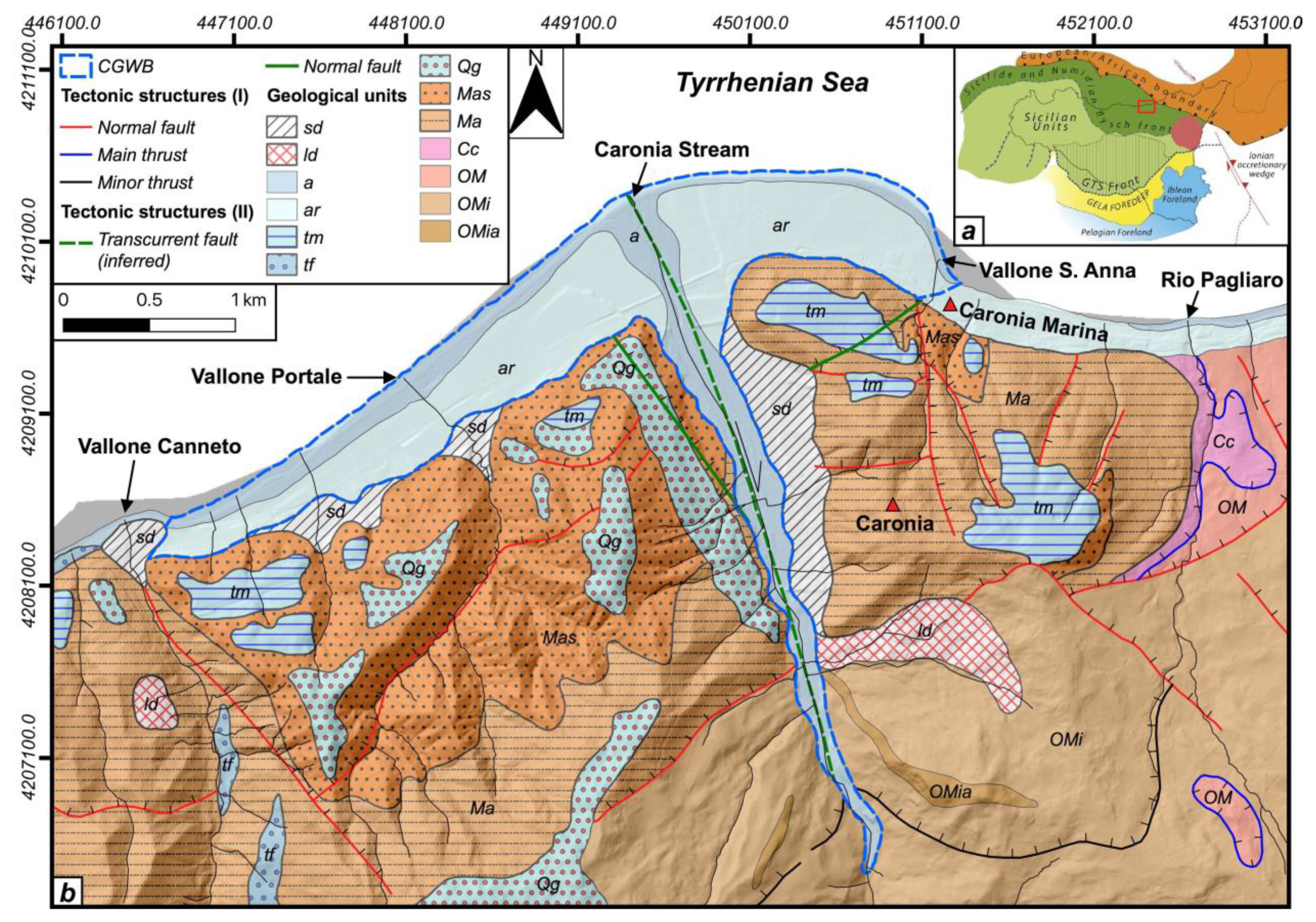
2.1. Geomorphological and Geological Setting

The Caronia Groundwater Body (CGWB) is located on the northern Sicilian coast, near the Caronia village. The CGWB falls in the north-eastern sector of the Nebrodi Mounts, representing a morphologically and geologically important area, adjacent to the orographic boundary between the Nebrodi and Peloritani Mounts.
Sicily is located in the central-western Mediterranean region, at the boundary between the African and European plates, and represents the connecting element between the African Maghrebian and the Southern Apennine Chains [60,61,62,63]. As part of the Appennine-Tyrrhenian System, the geological setting of Sicily (Figure 1a) is characterized by very articulate “collisional” complex (Figure 1a), which presents the typical configuration of a foreland–foredeep–chain system [63,64,65,66]. The growth of this complex, led by the convergence between African and European plates and the coeval roll-back of the subduction hinge of the Ionian Slab (Figure 1a), started in the late Oligocene-early Miocene and persisted through different tectonic phases (compressional, extensional, and transcurrent) until the late Quaternary [60,62,67,68].
The upstream sector of the CGWB area is characterized by smoothed outline hills, formed in the flyschoid sedimentary sequences and dissected by a narrow streambed, which gradually widens towards the mouth area. The river presents a characteristic delta shape, on which a wide coastal and alluvial plain rises.
The Nebrodi Mountains, together with the Peloritani Mountains, occupy the central-eastern sector of the Sicilian Maghrebian Chain (SMC), which represents the orogenic domain of the so-called “collisional” complex of Sicily [60,62,67,68,69,70,71,72,73,74]. In particular, the Sicilian orogen presents the maximum axial depression in the north-eastern sector [68], through a first-order thrust surface. This important structure, known as “Taormina Line” [75,76], outcrops along the San Fratello-Alcantara alignment, where the overlap of the Peloritani Tectonic Units on the Nebrodi ones occurs [61].
Furthermore, the SMC is also displaced and fragmented by a complex strike- and dip-slip “Neotectonic” fault grid (Plio-Quaternary), expressed by right-lateral, synthetic, NW–SE and W–E oriented, and left-lateral, antithetic, NE–SW and N–S oriented structures [68,77,78,79,80]. This complicated structural setting is well observable in the Caronia area (Figure 1b) [72], where recent high-angle normal and transcurrent faults are present, often reactivating and re-orienting older fault surfaces [61,68,72,76].
The tectono-stratigraphic sequence outcropping in the area adjacent to the CGWB (Nebrodi Mts.) consists of units derived from the deformation of the so-called Sicilide [81] and Numidian domains [82,83,84], generally detached from their original substrate and dismembered in first-order tectonic units, unconformably covered by early-middle Miocene thrust-top basin deposits and by Plio-Quaternary marine, transitional, and continental successions, as shown in Figure 1b [61,72,76,85,86].
Figure 1. Geological sketch map of the area adjacent to the CGWB (blue dashed line). Inside (a), the tectonic map illustrating the main elements of the “collisional” complex of Sicily. The geological sketch map (b) was elaborated with GIS software (QGIS 3.16), using a DEM image as topographic support. The stratigraphic and tectonic information for this map are derived from previous work [85] and from the official geological map [86], as well as from the accompanying explanatory notes [61,76]. Moreover, the tectonic structures described by previous authors [76,85] are reported as I in this map, while those derived from the official geological chart [86] are indicated as II. OMi-Omia = Numidian Flysch-Monte Maragone Tectonic Unit; OM = Numidian Flysch-Monte Salici-Monte Castelli Tectonic Unit; Cc = “Argille Scagliose Superiori” Tectonic Unit; Ma = Reitano Flysch; Mas = Reitano Flysch “Conglomerati di Caronia” Member; Qg = “Ghiaie e sabbie di Messina”; tf = stream terrace deposits; tm = marine terrace deposits; ar = recent alluvial deposits; a = present alluvial deposits; ld = landslide deposits; sd = slope deposits.
Water 15 03206 g001

2.2. Hydrogeological Setting

Starting from the analysis of the Potential Infiltration Coefficients [8,41,87], it is observed that the lithotypes with higher permeability are concentrated along the coastal plain and the Caronia stream. These sectors are entirely characterized by recent alluvial deposits and middle-late Quaternary deposits, mainly consisting of gravels, sands, and silts (Figure 1b) [61,76]. These lithotypes are characterized by a high permeability due to primary porosity and generally host unconfined aquifers, with transmissivity increasing in the direction of the outlet of the rivers and on the coastal plains, proportionally with the increase in the thickness of the aquifer [15,88]. These types of aquifers are generically in hydraulic connection with the recharging areas to the coastal plains [3,15,89,90]. Despite having a low capacitive role, due to its limited extension, the CGWB has been considered to be able to satisfy the local water needs (INGV-DAR 2019).
The CGWB is hydrogeologically superimposed on flyschoid lithotypes with lower permeability [91]. Laterally, with the exception of the northern margin represented by the sea, the CGWB is delimited by boundaries with no or very low flow, represented by the flyschoid lithotypes of the Reitano-Monte Castellaci and Pizzo Michele-Monte Castelli [41,59]. Regarding the hydrogeological characteristics of the lithotypes outcropping in the CGWB [92,93,94], the following hydrogeological complexes have been distinguished [41,91,95,96]:
  • Present and recent alluvial hydrogeological complex (Holocene): deposits with high permeability (10−2 m/s > k > 10−4 m/s) which form the main part of the CGWB, extending in length for about 6 km and just under a kilometer wide.
  • Hydrogeological complex constituted by river and marine terrace deposits (middle-late Pleistocene) and “Ghiaie e sabbie di Messina” (middle Pleistocene): it does not outcrop as it is covered by recent alluvial deposits. These deposits have high permeability (10−2 m/s > k > 10−4 m/s) due to primary porosity, even if very heterogeneous.
  • Hydrogeological complex of the Reitano Flysch (early-middle Miocene): it presents localized and variable permeability, mainly due to fracturing. It is composed of micaceous sandstone and lithic arkoses with medium-large grain, lightly cemented, with decimetric intercalations of silty-clays. In the upper part of this complex, decametric conglomeratic bodies relative to the so-called “Conglomerati di Caronia”, intercalated with the arenaceous deposits of Reitano Flysch, are often present. These lithotypes vary from moderately permeable (10−4 m/s > k > 10−5 m/s) to semi-permeable (10−6 m/s > k > 10−7 m/s) and constitute the main substrate of the CGWB.
  • Hydrogeological complex of the Numidian Flysch belonging to the Monte Maragone Unit (Late Oligocene-early Miocene): it consists of argillites alternated with silty-clays, followed upwards by quartzarenites and quartzosiltites in large banks. These lithotypes have low and very low permeability (10−7 m/s > k> 10−9 m/s). For these characteristics, the Numidian Flysch deposits constitute the impermeable substrate of the southernmost part of CGWB.

3. Materials and Methods

3.1. Previous Geognostic and Geophysical Investigation

Six boreholes, falling within the studied area, were analyzed in order to better characterize the alluvial deposits and geological substrate features and thickness (Figure 2). Four of these boreholes (BH1, BH2, BH3, and BH6) were drilled using the core destruction method, in relation to the geological and hydrogeological surveys for the construction of an aqueduct between the villages of Santo Stefano di Camastra and Caronia. The remaining two boreholes (BH4 and BH5) were instead drilled using the continuous coring method, during the geological surveys for the construction of the A20 highway (Palermo-Messina). Similar stratigraphic succession was found in the analyzed boreholes, except for the BH2 entirely drilled in the alluvial deposits of the Caronia River (up to 25 m depth). In the other boreholes, the cumulative thickness of the alluvial deposits ranges from a minimum of 9 m up to a maximum of 15 m (Figure 2). Below the alluvial deposits, arkoses interbedded with silty clays are present. These latter deposits, ascribed to the Reitano Flysch, often present a surface-deteriorated and -fractured cap, the thickness of which varies between 4 and 5 m. In general, the maximum thickness of the Reitano Flysch deposits, observed in the analyzed boreholes, ranges between 8 and 29 m (Figure 2).
Geoelectric surveys and seismic refraction surveys (Figure 3) were realized within the Caronia water body in the 1970s in order to describe the aquifer present in the Caronia area. These acquisitions were made as part of a project sponsored by [97] CASMEZ (1978). This project produced maps concerning the geophysical (geoelectric and seismic) characterization of the area. In particular, 17 vertical electrical sounding (VES) and three refraction seismic lines were carried out inside the CGWB. Each line consists of several segments of measurements arranged in continuity.
The seismic lines were positioned, distancing them from each other by about 200 m, along a direction almost perpendicular to the axis of the Caronia stream so as to intercept increasing volumes of alluvial deposits proceeding from upstream to downstream. The seismic refraction data show a two-layer model, with the thickness of the first layer varying from a few meters up to a maximum of 30 m in the northernmost area. However, original data were not available and only interpretive models could be evaluated.

3.2. New Processing and Interpretation of Vertical Electrical Soundings

Although the vertical electrical sounding (VES) technique allows, in theory, the solution of the inverse problem for electrical resistivity one-dimensional models, in many cases this method is applied to reconstruct 3D resistivity models in the subsoil, through the interpolation of 1D models which are mutually constrained, each with the adjacent models, compatibly with the tectonic structures present in the studied area. Practically, during the interpolation phase, optimization criteria must be followed to guarantee the acceptability of the model from a geological point of view. In fact, especially for large-scale geoelectric investigations, the application of 2D and 3D techniques is often impractical, for economic or logistical reasons, as the data acquisition would be impracticable or at least considerably difficult to carry out.
The use of this method of reconstruction is advisable only when the resistivity gradient is small along the directions parallel to the ground surface. In these cases, therefore, 2D or 3D resistivity models can be made by performing VES surveys on more or less regular meshes or along profiles, possibly reserving the application of 2D and 3D acquisition techniques to sectors of limited extension within the investigation area, when the resistivity varies with high horizontal gradients.
All the VESs collected were available only in paper format, given only by the graph of the apparent resistivity curves as a function of the half-distance AB/2 between the current electrodes. For each VES, an ASCII file was created containing the geographic coordinates and the altitude of the center of the survey, the array type, the number of measurements considered for each curve (corresponding to the number of points picked on the graph), and, for each measurement, the value of AB/2 and apparent resistivity.
Subsequently, using a MATLAB script, data were imported into the ZondIP1D software (v. 5.2) and converted into the proprietary format. By grouping them into a single database, all the VESs were carried out within the water body of the Caronia torrent.
ZondIP1D software allowed inversions with the least squares method. The inversions were carried out taking care to limit the lateral heterogeneities and constraining the inversions, where possible, with coring stratigraphic data. In the areas characterized by quite regular geological structures, a 1.5D inversion algorithm was used, in which the deeper layer of the resistivity section is considered almost horizontal, while the most superficial layers of the section can have sharper lateral variations. In consideration of this, a window comprising three or more adjacent VESs is inverted simultaneously, giving greater weight to the points of the central curve for the poorly fitting calculation.
The 1D inverse models obtained were therefore interpolated with each other to derive the electrical resistivity sections (Figure 4). The choice of the section traces was made considering the VES areal distribution and, at the same time, the shape of the geological structures.
The preliminary resistivity sections were useful for the making of the geological sections of the river basin. In fact, from the analysis of these resistivity sections, a first description of the characteristics of the subsoil was obtained within the Caronia water body. A preliminary geological interpretation was given to each “resistivity pattern” recognized in the sections, based on the mapped lithology and the geometry of the sedimentary bodies expected, given the structural and geomorphological asset of the area.

3.3. New Geophysical Surveys

Previous geophysical studies were improved with new geophysical measurements to define with greater precision the depth of the substrate of the groundwater body and the thicknesses of the lithologies present in the subsoil. The new geophysical data were acquired with active seismic techniques using the Multichannel Analysis of the Surface Waves (MASW) technique and microtremor recordings elaborated with the horizontal-to-vertical spectral ratio (HVSR) technique. The location of seismic investigations was based on the position of previous investigations, with the aim of integrating the available data mesh (Figure 3). The HVSR (horizontal-to-vertical spectral ratio) methodology [45,98] is a useful technique for the analysis of seismic noise. This methodology consists of calculating the ratio between the horizontal components with respect to the vertical component of the spectrum of seismic ambient noise. A 3D velocimeter records microtremor signals along the three directions and the H/V spectral ratio is calculated. The inversion of this curve returns an S-wave velocity profile and can be used to recover stratigraphical information if the inversion process is constrained by some other variable and soil features.
An total of 15 seismic microtremor acquisitions were made using a 3D velocimeter specially designed for ambient noise studies. This instrument provides good accuracy in the frequency range from 0.1 to about 30 Hz. The location of the seismic microtremor measures concerned not only the main arm of the water body but also the area of the flood plain, where other acquisitions were realized both on the left hydrographic and on the right hydrographic of the Caronia torrent. The duration of each ambient noise recording was 18 min.
MASW methodology [43] is based on the analysis of the surface waves dispersion curve. This is derived by picking the maximum oscillation on the phase velocity vs. frequency graph, derived by applying a Fourier transform to seismic signals registered at the geophones. The seismic source is generated by a heavy sledgehammer, which hits the ground at a determined offset from the geophone spread. The dispersion curve obtained is inverted by starting from an initial conceivable S-wave velocity model and solving the inverse problem via the Gauss–Newton least squares inversion algorithm.
Four MASW surveys were carried out to obtain more detailed information on the trend of Vs near surface and to constrain the inversion of the HVSR curves [53]. Indeed, constraining the HVSR inversion with independent parameters, such as shear wave velocity or the thickness of upper layers derived from MASW inversion, is useful for reducing the number of equivalent inverse HVSR models. In this way, four active seismic measurements were selected in correspondence with the same number of HVSR measurements chosen in different positions of the Caronia water body, and their inverse models served to constrain the most superficial part of the corresponding inverse HVSR models.
MASW surveys were carried out along the road of the Caronia stream and in the coastal plain, at four points distant from each other in an attempt to better describe the changes in S-wave velocity and in flood thickness along the river path (Figure 5).
All acquisitions were realized using a high-resolution multichannel seismograph. The MASW array generally consisted of twelve 4.5 Hz vertical geophones, 2 m spaced and at an offset of 5 m. A single measurement (MASW 3) was carried out using 24 vertical geophones spaced 2 m and at an offset of 8 m. HVSR surveys carried out in the water body were divided into clusters on the basis of their geographical proximity and lithological similarity to the nearest MASW survey, whose inverse model was used as a constraint.

4. Results and Discussion

4.1. MASW and HVSR Results

MASW results show the velocity of the S-wave compatible with the outcropping succession present in the investigated sites (Figure 5). MASW 2, 3, and 4, carried out along the main axis of the Caronia torrent from the southern sector towards the north, show an average velocity value equal to 259 m/s, attributed to the current alluvial deposits.
Results of 15 seismic passive measurements (HVSR), constrained by four MASW acquisitions, allowed reconstruction of seismostratigraphic patterns. Figure 6 shows the HVSR curves related to those measures carried out near the four MASW surveys, whereas their inverse 1D models, constrained by the corresponding MASW models, are presented in Figure 7.
Referring to these models, a seismostratigraphic level is shown with an average value of 272 m/s for the top of the sedimentary deposits. The thickness of this upper layer varies from 1.5 m to 4 m. Based on the geological survey, these Vs characteristics can be associated with the alluvial deposits located near the current river for HVSR 12, HVSR 14, and HVSR 15. Very similar Vs features have been described in previous works: similar values, slightly higher and confirmed to 300 m/s, have been reported for conglomerates, gravels, and sands from alluvial deposits [99]. The lowest shear wave velocity calculated for this upper layer corresponds to values close to 180 m/s, as shown for HVSR 13. This latter value is attributable to the recent alluvial plain deposits present in the wide plain next to the sea. A second deeper seismostratigraphic level is recognized for each of the four HVSR models shown in Figure 7. For this layer, Vs varies from 300 to 500 m/s. Its thickness varies from 10 m in HVSR 15 to 25 m in HVSR 12. This layer could be associated with permeable non-surfacing alluvial deposits. These would constitute the largest volume of the CWB.
A third layer is characterized by a higher S-wave velocity, ranging from 400 m/s to 800 m/s. The thickness of this layer is greater in HVSR 13, where it is equal to 30 m. The Vs values are attributable to the Reitano Flysch. The wide range of velocities of this layer is due to the heterogeneous nature of these deposits, which are more altered in the upper part and more compact in depth.
A last seismic stratigraphic layer is present in all velocity models except HVSR 13. Resulting velocities between 900 and 1000 m/s could be associated with clayey deposits of varicolored clays.

4.2. A Tridimensional Model of the Electrical Resistivity

The inverse models of electrical resistivity, obtained by the above-discussed re-inversion of the available VES in the area, were interpolated using Voxler software (Golden Software, v. 4.0), to obtain a 3D graphic representation of the trend of electrical resistivity. This is limited at the top by the Digital Elevation Model of the area, at the sides by the boundaries of the water body, and at the base by the depths of the investigation reached by each VES (Figure 8). To take into account the high contrasts of the geophysical parameter, the logarithm of electrical resistivity was preferred.
The tridimensional model describes the presence of a resistive overburden (60–80 Ωm), interpreted as alluvial materials, above a conductive substrate (7–20 Ωm), corresponding to the clayey-marly matrix soils of the Reitano Flysch surfacing near the river. In order to have a clearer view of the electrical resistivity trend within the model, horizontal slices were extracted at predefined levels below sea level. Two of them are presented and discussed here as examples. The first horizontal slice at 25 m b.s.l. (Figure 8b) shows high values of resistivity at the possible marine intrusion (therefore located in the most superficial portion) and a strong contrast of resistivity located at a transcurrent fault in evidence in the mountain zone. The second slice at 80 m b.s.l. (Figure 8c) instead shows very low resistivity values in the north-eastern part. This could be indicative of a marine intrusion phenomenon, probably located in the most porous portion of the alluvial material of the plain.
Starting from the 3D model, two vertical sections are also presented, useful for geological interpretation. The first section (A-A’) extends for 4400 m along the coastal strip, in a direction subparallel to the coastline. The second section (B-B’) extends along the axis of the stream for a length of 2300 m (Figure 9). The location of the two sections is shown in Figure 3.
The electrical resistivity features of the sedimentary deposits observable in sections A-A’ and B-B’ show horizontal and vertical variations, ranging from 20 to 500 Ωm (Figure 9). In particular, these electrical resistivity variations allowed different horizons and layers to be distinguished (Figure 9). These latter features, characterized by precise resistivity values, were attributed to the geological deposits outcropping around the Caronia area (Figure 1) and used to reconstruct the stratigraphic and structural setting.
From the bottom to the top of the two sections, layer f, with resistivity values of about 40 Ωm, could refer to the clays and marls of the “Argille Scagliose Superiori” unit, outcropping to the east of the Caronia area. This layer has been continuously recognized in section A-A’ and only in the northernmost part of section B-B’. Above these deposits, the increasing resistivity values, here identified by the layer d (60–100 Ωm), can be associated with the arenaceous facies with intercalations of silty-clays belonging to the Reitano Flysch formation. In this view, layers labeled e (50–60 Ω m) could represent thicker clayey portions of the Miocene lithological unit. The highest resistivity value portions (200–500 Ω m) observed in both sections, named layer b, can be related to the “Conglomerati di Caronia” member deposits and/or to conglomeratic channeled structures in correspondence with the central sector of the streambed. From another point of view, these high resistivity values, coinciding with the mouth sector of the Caronia stream, could also indicate the presence of freshwaters flowing below the streambed. The low resistivity lenticular and cuneiform bodies (20–40 Ω m) observed in both sections, named layer c, probably describe the seawater intrusion in the Caronia sedimentary succession, in correspondence with sectors with high porosity and/or minor freshwater hydraulic load. Finally, observing the BH1 and BH3 stratigraphic logs and the resistivity values (40–70 Ωm), the uppermost layer a was ascribed to the alluvial deposits, filling the Caronia streambed and the relative coastal plain.
The three stepped forms recognized in the sections (Figure 6), indicated by red dashed lines, could represent normal tectonic structures. These faults are compatible in terms of location, shape, and type of dislocation with those recognized and already mapped [86] (APAT, 2013) in the hills immediately west and east to the terminal part of the Caronia stream valley, and with the inferred transtensional structure where the streambed develops (Figure 1). Moreover, this latter structure could also be responsible for the thickening of the succession, especially as regard to layers a and b, in correspondence with the central sector of the Caronia stream mouth (Figure 9). In this view, space created by the net-slip movement linked to this fault may have been gradually filled by Reitano Flysch conglomeratic bodies (i.e., “Conglomerati di Caronia” member and/or channeled structures) and by Quaternary deposits.

4.3. Estimate of the Bottom of the CGWB

All the geophysical surveys performed (VES, SR, HVSR, and MASW) were geologically interpreted using the stratigraphic logs (from BH1 to BH6) as calibration. This made it possible to transform the information of the geophysical parameters in terms of the thickness of the water body in the investigated points. These values were interpolated by applying a kriging-type algorithm using the Surfer software (v. 18). In correspondence with the water body superficial limit, the thickness of the groundwater body was set equal to zero. The resulting thickness map (Figure 10a) shows two areas with significant thicknesses: the smallest is located in the extreme eastern portion, where 30 m thicknesses are reached; the largest is located west of the current delta, where thicknesses reach about 40 m. This part coincides with the area already identified as a transcurrent fault in the 3D resistivity model. The thicknesses of the CGWB are larger in the eastern part of this probable fault area.
Furthermore, the bottom of the water body was rebuilt (Figure 10b) because it is needed as an input for the construction of a mathematical flow model.

4.4. Numerical Flow Model for the CGWB

The reconstruction of the lower boundary of the water body plays a key role in the construction of the mathematical model of static flow. This was carried out to implement the hydrogeological model of the CGWB. The finite difference calculation code MODFLOW [100] in steady state was used to create the flow model. This kind of analysis solves the groundwater flow differential equation using the finite difference approach within the groundwater systems through a gridded spatial discretization [101]. In order to create a numerical model, which describes the hypothetical trend of flow within a groundwater body, it is necessary to define the model in the spatial domain. This must be divided into cells, to each of which is assigned both the initial and boundary conditions and the physical and hydrogeological properties. These conditions and properties are considered homogeneous within the cell itself, and attributed to the center of the cell [102].
The sectors considered by the numerical flow model correspond to the coastal plain and the Caronia stream mouth. In the first phase, the top and bottom levels were defined. For the top, corresponding to the topographic surface, altitudes derived from the DEM of Sicily were assumed. The hydrogeological substrate, defined in the digital model of the CGWB, was adopted as the bottom of the flow model. For the horizontal discretization, the modeled area (coastal plain) was subdivided using a mesh of 50 × 50 m cells, while 12 layers were identified for the vertical subdivision (Figure 11). Subsequently, the hydrogeological properties were defined to be assigned to the various sectors of the model. Hydraulic conductivity values along the three spatial directions (Kx = 3.5 × 10⁻⁵ m/s, Ky = 3.5 × 10⁻⁵ m/s, and Kz = 3.5 × 10⁻⁶ m/s) were attributed to layers 1 to 11, describing the part of the succession in which the groundwater flows. Finally, layer 12, corresponding to the bottom, was defined as null flow. A further step for the realization of a flow model is related to the definition of the boundary conditions [103].
These features define the physical constraints in the perimeter cells that are imposed on the flow model (Figure 11). As boundary conditions, the following parameters were adopted:
(A)
Refill value: 161 mm/year for 365 days. This refill was applied only to layer 1, which defines the portion of the model identifiable with the topographic surface.
(B)
Constant load: An area representing the portion of the model (red cells in Figure 11) where the flow stops being considered as having a constant hydraulic load. It was defined by assigning the value 0 to the coastline downstream of the domain.
(C)
Top-up refill: This parameter represents the sub-alveal contributions. This feature describes the direct contributions provided by the upstream hydrological basin. These values were assigned, as saturated cells (green cells in Figure 11), corresponding to the groundwater depth measured in the observation well n.5.
(D)
The area outside the modeled area was considered to be zero flow (gray sectors in Figure 11).
The mathematical model obtained was finally calibrated and validated thanks to the piezometric values detected during the field activities performed in the area under study. Four wells were considered, one of which (OW 5) was inside the Caronia streambed. These wells have an undisturbed piezometric level and are sufficiently far from other wells in use. The simulation results are shown in Figure 12. The trend of the simulated piezometry shows how the aquifer is fed by the inputs coming from the mountain. Furthermore, the stream portion considered in this model provides an important contribution to feed the coastal plain aquifer.
Finally, the calculated vs. observed piezometric values are shown in Figure 13. A normalized RMS of 7.49% is obtained, with an average square deviation of 0.63 m. This is considered to be an acceptable value considering the width of the simulated area.

5. Conclusions

The characterization of the Caronia Groundwater Body (CGWB), in north-eastern Sicily, was realized thanks to the construction of a conceptual physical model and the related hydrogeological flow model, which is fundamental for the definition of monitoring programs, hydrogeological risk assessment, and correct water resources management.
A series of previous geophysical data (vertical electrical sounding surveys and refraction seismic profiles) were re-inverted using constraints obtained from stratigraphic data. The new geophysical models obtained, together with the information obtained from new surveys with surface wave and microtremor techniques (MASW and HVSR), made it possible to obtain three-dimensional models of physical parameters of the subsoil (electrical resistivity, seismic velocity of pressure, and shear waves). These models were used to define the depth of the bottom of the CGWB and the thickness of the alluvial deposits that characterize the streambed. This allowed shape, volume, and physical characteristics of the CGWB to be defined in sufficient detail. This numerical information served as a basis to generate a mathematical model of groundwater flow in order to simulate the spatial and temporal variability of the flow and, consequently, to make forecast estimates of the water supplies to the coastal plain. The underground flow model was preliminarily tested by comparing the theoretical results with some piezometric measurements performed. The main result of the calibration of the model was the refinement and validation of the assignment of the average hydrodynamic parameters of the modeled aquifer. In this way, it was possible to carry out realistic and reliable simulations of the underground flow in the CGWB. The results showed a good correspondence between predicted and observed data, confirming the reliability of the model obtained for the description of the aquifer dynamics.

Author Contributions

Conceptualization, P.C., R.M. and R.F.; Methodology, A.C., P.C., R.M. and A.B.; Software, R.M.; Validation, P.C. and R.M.; Formal analysis, A.C., P.C., R.M., A.B. and N.C.; Investigation, A.C., L.A. and A.B.; Data curation, P.C., R.M. and N.C.; Writing—original draft, A.C., P.C., R.M., L.A., A.B. and N.C.; Writing—review & editing, A.C., P.C., R.M. and A.B.; Visualization, A.C. and R.M.; Supervision, P.C. and R.F.; Project administration, R.F.; Funding acquisition, R.F. All authors have read and agreed to the published version of the manuscript.

Funding

This research was funded by Regione Siciliana, Commissario Delegato per l’Emergenza Bonifiche e la tutela delle Acque in Sicilia.

Data Availability Statement

Not applicable.

Conflicts of Interest

The authors declare no conflict of interest.

References

  1. Chenini, I.; Zghibi, A.; Kouzana, L. Hydrogeological investigations and groundwater vulnerability assessment and mapping for groundwater resource protection and management: State of the art and a case study. J. Afr. Earth Sci. 2015, 109, 11–26. [Google Scholar] [CrossRef]
  2. Erdoğan, M.; Karagüzel, R. A new hydrogeologically based approach to determining protected areas in drinking water supply reservoirs: A case study in the Ağlasun sub-basin (Burdur, Turkey). Environ. Earth Sci. 2016, 75, 126. [Google Scholar] [CrossRef]
  3. Käser, D.; Hunkeler, D. Contribution of alluvial groundwater to the outflow of mountainous catchments. Water Resour. Res. 2016, 52, 680–697. [Google Scholar] [CrossRef]
  4. Paillet, F.L.; Reese, R.S. Integrating Borehole Logs and Aquifer Tests in Aquifer Characterization. Groundwater 2000, 38, 713–725. [Google Scholar] [CrossRef]
  5. Zuffetti, C.; Comunian, A.; Bersezio, R.; Renard, P. A new perspective to model subsurface stratigraphy in alluvial hydrogeological basins, introducing geological hierarchy and relative chronology. Comput. Geosci. 2020, 140, 104506. [Google Scholar] [CrossRef]
  6. Straface, S.; Yeh, T.-C.J.; Zhu, J.; Troisi, S.; Lee, C.H. Sequential aquifer tests at a well field, Montalto Uffugo Scalo, Italy. Water Resour. Res. 2007, 43. [Google Scholar] [CrossRef]
  7. Alexander, M.; Berg, S.J.; Illman, W.A. Field Study of Hydrogeologic Characterization Methods in a Heterogeneous Aquifer. Groundwater 2011, 49, 365–382. [Google Scholar] [CrossRef]
  8. Fontana, M.; Grassa, F.; Cusimano, G.; Favara, R.; Hauser, S.; Scaletta, C. Geochemistry and potential use of groundwater in the Rocca Busambra area (Sicily, Italy). Environ. Geol. 2008, 57, 885–898. [Google Scholar] [CrossRef]
  9. Cangemi, M.; Madonia, P.; Albano, L.; Bonfardeci, A.; Di Figlia, M.G.; Di Martino, R.M.R.; Nicolosi, M.; Favara, R. Heavy Metal Concentrations in the Groundwater of the Barcellona-Milazzo Plain (Italy): Contributions from Geogenic and Anthropogenic Sources. Int. J. Environ. Res. Public Health 2019, 16, 285. [Google Scholar] [CrossRef]
  10. Chen, Q.; Jia, C.; Wei, J.; Dong, F.; Yang, W.; Hao, D.; Jia, Z.; Ji, Y. Geochemical process of groundwater fluoride evolution along global coastal plains: Evidence from the comparison in seawater intrusion area and soil salinization area. Chem. Geol. 2020, 552, 119779. [Google Scholar] [CrossRef]
  11. Massey, A.C.; Taylor, G.K. Coastal evolution in south-west England, United Kingdom: An enhanced reconstruction using geophysical surveys. Mar. Geol. 2007, 245, 123–140. [Google Scholar] [CrossRef]
  12. Sauret, E.S.G.; Beaujean, J.; Nguyen, F.; Wildemeersch, S.; Brouyere, S. Characterization of superficial deposits using electrical resistivity tomography (ERT) and horizontal-to-vertical spectral ratio (HVSR) geophysical methods: A case study. J. Appl. Geophys. 2015, 121, 140–148. [Google Scholar] [CrossRef]
  13. Larkin, R.G.; Sharp, J.M., Jr. On the relationship between river-basin geomorphology, aquifer hydraulics, and ground-water flow direction in alluvial aquifers. Geol. Soc. Am. Bull. 1992, 104, 1608–1620. [Google Scholar] [CrossRef]
  14. Gregory, K.; Benito, G.; Downs, P. Applying fluvial geomorphology to river channel management: Background for progress towards a palaeohydrology protocol. Geomorphology 2008, 98, 153–172. [Google Scholar] [CrossRef]
  15. Cimino, A.; Cosentino, C.; Oieni, A.; Tranchina, L. A geophysical and geochemical approach for seawater intrusion assessment in the Acquedolci coastal aquifer (Northern Sicily). Environ. Geol. 2007, 55, 1473–1482. [Google Scholar] [CrossRef]
  16. Hamzah, U.; Samsudin, A.R.; Malim, E.P. Groundwater investigation in Kuala Selangor using vertical electrical sounding (VES) surveys. Environ. Geol. 2006, 51, 1349–1359. [Google Scholar] [CrossRef]
  17. Alile, O.M.; Ujuanbi, O.; Evbuomwan, I.A. Geoelectric investigation of groundwater in Obaretin Iyanomon locality, Edo state, Nigeria. J. Geol. Min. Res. 2011, 3, 13–20. [Google Scholar] [CrossRef]
  18. Coker, J.O. Vertical electrical sounding (VES) methods to delineate potential groundwater aquifers in Akobo area, Ibadan, South-western, Nigeria. J. Geol. Min. Res. 2012, 4, 35–42. [Google Scholar] [CrossRef]
  19. Fadele, S.I.; Sule, P.O.; Dewu, B.B.M. The use of vertical electrical sounding (VES) for groundwater exploration around Nigerian College of Aviation Technology (NCAT), Zaria, Kaduna State, Nigeria. Pac. J. Sci. Technol. 2013, 14, 549–555. [Google Scholar]
  20. Abdullahi, M.G.; Toriman, M.E.; Gasim, M.B. The Application of Vertical Electrical Sounding (VES) for Groundwater Exploration in Tudun Wada Kano State, Nigeria. J. Geol. Geosci. 2015, 4, 1–3. [Google Scholar] [CrossRef]
  21. van Overmeeren, R.A. A combination of electrical resistivity, seismic refraction, and gravity measurements for groundwater exploration in Sudan. Geophysics 1981, 46, 1304–1313. [Google Scholar] [CrossRef]
  22. Haeni, F.P. Application of seismic refraction methods in groundwater modeling studies in New England. Geophysics 1986, 51, 236–249. [Google Scholar] [CrossRef]
  23. Grelle, G.; Guadagno, F.M. Seismic refraction methodology for groundwater level determination: “Water seismic index”. J. Appl. Geophys. 2009, 68, 301–320. [Google Scholar] [CrossRef]
  24. Dafflon, B.; Irving, J.; Holliger, K. Use of high-resolution geophysical data to characterize heterogeneous aquifers: Influence of data integration method on hydrological predictions. Water Resour. Res. 2009, 45. [Google Scholar] [CrossRef]
  25. Khan, U.; Faheem, H.; Jiang, Z.; Wajid, M.; Younas, M.; Zhang, B. Integrating a GIS-Based Multi-Influence Factors Model with Hydro-Geophysical Exploration for Groundwater Potential and Hydrogeological Assessment: A Case Study in the Karak Watershed, Northern Pakistan. Water 2021, 13, 1255. [Google Scholar] [CrossRef]
  26. Bowling, J.C.; Rodriguez, A.B.; Harry, D.L.; Zheng, C. Delineating Alluvial Aquifer Heterogeneity Using Resistivity and GPR Data. Groundwater 2005, 43, 890–903. [Google Scholar] [CrossRef]
  27. Kim, J.-W.; Choi, H.; Lee, J.-Y. Characterization of hydrogeologic properties for a multi-layered alluvial aquifer using hydraulic and tracer tests and electrical resistivity survey. Environ. Geol. 2005, 48, 991–1001. [Google Scholar] [CrossRef]
  28. Goldman, M.; Kafri, U. Hydrogeophysical Applications in Coastal Aquifers. In Applied Hydrogeophysics; Springer: Dordrecht, The Netherlands, 2007; pp. 233–254. [Google Scholar] [CrossRef]
  29. Wattanasen, K.; Elming, S. Direct and indirect methods for groundwater investigations: A case-study of MRS and VES in the southern part of Sweden. J. Appl. Geophys. 2008, 66, 104–117. [Google Scholar] [CrossRef]
  30. Doro, K.O.; Leven, C.; Cirpka, O.A. Delineating subsurface heterogeneity at a loop of River Steinlach using geophysical and hydrogeological methods. Environ. Earth Sci. 2013, 69, 335–348. [Google Scholar] [CrossRef]
  31. Dickson, N.E.M.; Comte, J.-C.; McKinley, J.; Ofterdinger, U. Coupling ground and airborne geophysical data with upscaling techniques for regional groundwater modeling of heterogeneous aquifers: Case study of a sedimentary aquifer intruded by volcanic dykes in Northern Ireland. Water Resour. Res. 2014, 50, 7984–8001. [Google Scholar] [CrossRef]
  32. Vilhelmsen, T.N.; Behroozmand, A.A.; Christensen, S.; Nielsen, T.H. Joint inversion of aquifer test, MRS, and TEM data. Water Resour. Res. 2014, 50, 3956–3975. [Google Scholar] [CrossRef]
  33. Michael, H.A.; Post, V.E.A.; Wilson, A.M.; Werner, A.D. Science, society, and the coastal groundwater squeeze. Water Resour. Res. 2017, 53, 2610–2617. [Google Scholar] [CrossRef]
  34. Daniels, J.J.; Roberts, R.; Vendl, M. Ground penetrating radar for the detection of liquid contaminants. J. Appl. Geophys. 1995, 33, 195–207. [Google Scholar] [CrossRef]
  35. Benson, A.K.; Payne, K.L.; Stubben, M.A. Mapping groundwater contamination using dc resistivity and VLF geophysical methods–A case study. Geophysics 1997, 62, 80–86. [Google Scholar] [CrossRef]
  36. Frohlich, R.K.; Urish, D.W.; Fuller, J.; O’Reilly, M. Use of geoelectrical methods in groundwater pollution surveys in a coastal environment. J. Appl. Geophys. 1994, 32, 139–154. [Google Scholar] [CrossRef]
  37. Cosentino, P.; Capizzi, P.; Fiandaca, G.; Martorana, R.; Messina, P.; Pellerito, S. Study and Monitoring of Salt Water Intrusion in The Coastal Area Between Mazara Del Vallo And Marsala (South-Western Sicily). In Methods and Tools for Drought Analysis and Management; Springer: Berlin/Heidelberg, Germany, 2007; pp. 303–321. [Google Scholar] [CrossRef]
  38. Capizzi, P.; Cellura, D.; Cosentino, P.; Fiandaca, G.; Martorana, R.; Messina, P.; Schiavone, S.; Valenza, M. Integrated hydrogeochemical and geophysical surveys for a study of sea-water intrusion. Boll. Geofis. Teor. Appl. 2010, 51, 285–300. [Google Scholar]
  39. Di Napoli, R.; Martorana, R.; Orsi, G.; Aiuppa, A.; Camarda, M.; De Gregorio, S.; Candela, E.G.; Luzio, D.; Messina, N.; Pecoraino, G.; et al. The structure of a hydrothermal system from an integrated geochemical, geophysical, and geological approach: The Ischia Island case study. Geochem. Geophys. Geosyst. 2011, 12. [Google Scholar] [CrossRef]
  40. Martorana, R.; Lombardo, L.; Messina, N.; Luzio, D. Integrated geophysical survey for 3D modelling of a coastal aquifer polluted by seawater. Near Surf. Geophys. 2013, 12, 45–59. [Google Scholar] [CrossRef]
  41. Capizzi, P.; Martorana, R.; Favara, R.; Albano, L.; Bonfardeci, A.; Catania, M.; Costa, N.; Gagliano, A. Geophysical Contribution to the Reconstruction of the Hydrological Model of “Barcellona-Milazzo Plain” Groundwater Body, Northen Sicily. In 25th European Meeting of Environmental and Engineering Geophysics; European Association of Geoscientists & Engineers: Moscow, Russia, 2019; pp. 1–5. [Google Scholar] [CrossRef]
  42. Paz, M.C.; Alcalá, F.J.; Medeiros, A.; Martínez-Pagán, P.; Pérez-Cuevas, J.; Ribeiro, L. Integrated MASW and ERT Imaging for Geological Definition of an Unconfined Alluvial Aquifer Sustaining a Coastal Groundwater-Dependent Ecosystem in Southwest Portugal. Appl. Sci. 2020, 10, 5905. [Google Scholar] [CrossRef]
  43. Park, C.B.; Miller, R.D.; Xia, J. Multimodal Analysis of High Frequency Surface Waves. In Proceedings of the Symposium on the Application of Geophysics to Engineering and Environmental Problems, Oakland, CA, USA, 14–18 June 1999. [Google Scholar]
  44. Alcalá, F.J.; Martínez-Pagán, P.; Paz, M.C.; Navarro, M.; Pérez-Cuevas, J.; Domingo, F. Combining of MASW and GPR Imaging and Hydrogeological Surveys for the Groundwater Resource Evaluation in a Coastal Urban Area in Southern Spain. Appl. Sci. 2021, 11, 3154. [Google Scholar] [CrossRef]
  45. Nakamura, Y. A method for dynamic characteristics estimation of subsurface using microtremor on the ground surface. Quat. Rep. Railw. 1989, 30, 25–33. [Google Scholar]
  46. Martorana, R.; Capizzi, P.; Avellone, G.; D’alessandro, A.; Siragusa, R.; Luzio, D. Assessment of a geological model by surface wave analyses. J. Geophys. Eng. 2016, 14, 159–172. [Google Scholar] [CrossRef]
  47. Martorana, R.; Agate, M.; Capizzi, P.; Cavera, F.; D’Alessandr, A. Seismo-stratigraphic model of “La Bandita” area in the Palermo Plain (Sicily, Italy) through HVSR inversion constrained by stratigraphic data. Ital. J. Geosci. 2018, 137, 73–86. [Google Scholar] [CrossRef]
  48. Sorensen, C.; Asten, M. Microtremor methods applied to groundwater studies. Explor. Geophys. 2007, 38, 125–131. [Google Scholar] [CrossRef]
  49. Delgado, J.; Casado, C.L.; Estévez, A.; Giner, J.; Cuenca, A.; Molina, S. Mapping soft soils in the Segura river valley (SE Spain): A case study of microtremors as an exploration tool. J. Appl. Geophys. 2000, 45, 19–32. [Google Scholar] [CrossRef]
  50. Martorana, R.; Capizzi, P.; D’Alessandro, A.; Luzio, D.; Di Stefano, P.; Renda, P.; Zarcone, G. Contribution of HVSR measures for seismic microzonation studies. Ann. Geophys. 2018, 61, 225. [Google Scholar] [CrossRef]
  51. Pino, P.; D’Amico, S.; Orecchio, B.; Presti, D.; Scolaro, S.; Torre, A.; Totaro, C.; Farrugia, D.; Neri, G. Integration of geological and geophysical data for revaluation of local seismic hazard and geological structure: The case study of Rometta, Sicily (Italy). Ann. Geophy. 2018, 61, SE227. [Google Scholar] [CrossRef]
  52. Scolaro, S.; Pino, P.; D’Amico, S.; Orecchio, B.; Presti, D.; Torre, A.; Totaro, C.; Farrugia, D.; Neri, G. Ambient noise measurements for preliminary microzoning studies in the city of Messina, Sicily. Ann. Geophys. 2018, 61, 228. [Google Scholar] [CrossRef]
  53. Dal Moro, G. Surface Wave Analysis for Near Surface Applications; Elsevier: Amsterdam, The Netherlands, 2014. [Google Scholar]
  54. Cafiso, F.; Canzoneri, A.; Capizzi, P.; Carollo, A.; Martorana, R.; Romano, F. Joint interpretation of electrical and seismic data aimed at modelling the foundation soils of the Maredolce monumental complex in Palermo (Italy). Archaeol. Prospect. 2020, 30, 69–85. [Google Scholar] [CrossRef]
  55. Gisser, M.; Sánchez, D.A. Competition versus optimal control in groundwater pumping. Water Resour. Res. 1980, 16, 638–642. [Google Scholar] [CrossRef]
  56. Percopo, C.; Brandolin, D.; Canepa, M.; Capodaglio, P.; Cipriano, G.; Gafà, R.; Iervolino, D.; Marcaccio, M.; Mazzola, M.; Mottola, A.; et al. Criteri tecnici per l’analisi dello stato quantitativo e il monitoraggio dei corpi idrici sotterranei. ISPRA Man. E Linee Guid. 2017, 157, 1–108. [Google Scholar]
  57. Heilweil, V.M.; Brooks, L.E. Conceptual Model of the Great Basin Carbonate and Alluvial Aquifer System: US Geological Survey Scientific Investigations Report; U.S. Geological Survey: Reston, VA, USA, 2011.
  58. Granata, A.; Castrianni, G.; Pasotti, L.; Gagliano Candela, E.; Scaletta, C.; Madonia, P.; Morici, S.; Bellomo, S.; La Pica, L.; Gagliano, A.L.; et al. Studio per la definizione dei modelli concettuali dei corpi idrici sotterranei di Peloritani, Nebrodi e ragusano e indagini geofisiche correlate. Atti del 37° Convegno del Gruppo Nazionale di Geofisica della Terra Solida-GNGTS. OGS 2018, 37, 104–108. [Google Scholar]
  59. Canzoneri, A.; Capizzi, P.; Martorana, R.; Albano, L.; Bonfardeci, A.; Costa, N.; Gagliano, A.L.; Favara, R. Modello idrogeoligoco del corpo idrico “Fiumara di Caronia” (Sicilia Settentrionale). Atti del 38°Convegno del Gruppo Nazionale di Geofisica della Terra Solida-GNGTS. OGS 2019, 38, 636–640. Available online: https://gngts.ogs.it/atti-del-38-convegno-nazionale-2/ (accessed on 1 July 2023).
  60. Catalano, R.; Di Stefano, P.; Sulli, A.; Vitale, F. Paleogeography and structure of the central Mediterranean: Sicily and its offshore area. Tectonophysics 1996, 260, 291–323. [Google Scholar] [CrossRef]
  61. Giunta, G.; Giorgianni, A. Note Illustrative del F.598 “S. Agata di Militello” Della Carta Geologica d’Italia Alla scala 1:50.000. SystemCart; ISPRA—Università degli Studi di Palermo: Rome, Italy, 2013. [Google Scholar]
  62. Catalano, R.; Valenti, V.; Albanese, C.; Accaino, F.; Sulli, A.; Tinivella, U.; Gasparo Morticelli, M.; Zanolla, C.; Giustiniani, M. Sicily’s fold/thrust belt and slab rollback: The SI.RI.PRO. seismic crustal transect. J. Geol. Soc. 2013, 170, 451–464. [Google Scholar] [CrossRef]
  63. Basilone, L. Lithostratigraphy of Sicily: UNIPA Springer Series; Springer International Publishing: Berlin/Heidelberg, Germany, 2018; pp. 1–349. [Google Scholar]
  64. Amodio-Morelli, L.; Bonardi, G.; Colonna, V.; Dietrich, D.; Giunta, G.; Ippolito, F.; Liguori, V.; Lorenzoni, F.; Paglionico, A.; Perrone, V.; et al. L’Arco Calabro-Peloritano nell’orogene Appenninico-Maghrebide. Mem. Soc. Geol. Ital. 1976, 17, 1–60. [Google Scholar]
  65. Bigi, G.; Cosentino, D.; Parotto, M.; Sartori, R.; Scandone, P. Structural Model of Italy (scale 1:500.000): Geodinamic Project: Consiglio Nazionale delle Ricerche, S.EL.CA: Rome, Italy. 1990. Available online: https://www.socgeol.it/438/structural-model-of-italy-scale-1-500-000.html/ (accessed on 1 July 2023).
  66. Giunta, G.; Nigro, F. Tectono-sedimentary constraints to the Oligocene-to-Miocene evolution of the Peloritani thrust belt (NE Sicily). Tectonophysics 1999, 315, 287–299. [Google Scholar] [CrossRef]
  67. Nigro, F.; Renda, P. Evoluzione geologica ed assetto strutturale della Sicilia centro- settentrionale. Boll. Soc. Geol. Ital. 1999, 118, 375–388. [Google Scholar]
  68. Giunta, G.; Luzio, D.; Agosta, F.; Calò, M.; Di Trapani, F.; Giorgianni, A.; Oliveri, E.; Orioli, S.; Perniciaro, M.; Vitale, M.; et al. An integrated approach to investigate the seismotectonics of northern Sicily and southern Tyrrhenian. Tectonophysics 2009, 476, 13–21. [Google Scholar] [CrossRef]
  69. Bianchi, F.; Carbone, S.; Grasso, M.; Invernizzi, G.; Lentini, F.; Longaretti, G.; Merlini, S.; Mostardini, F. Sicilia orientale: Profilo geologico Nebrodi-Iblei. Mem. Soc. Geol. Ital. 1987, 38, 429–458. [Google Scholar]
  70. Catalano, R.; Franchino, A.; Merlini, S.; Sulli, A. Central western Sicily structural setting interpreted from seismic reflection profiles. Mem. Soc. Geol. Ital. 2000, 55, 5–16. [Google Scholar]
  71. Catalano, R.; Gatti, V.; Avellone, G.; Basilone, L.; Frixa, A.; Ruspi, R.; Sulli, A. Subsurface Geometries in Central Sicily FTB as a Premise for Hydrocarbon Exploration. In Proceedings of the 70th EAGE Conference and Exhibition Incorporating SPE EUROPEC, Nuova Fiera Di Roma, Italy, 9–12 June 2008. [Google Scholar] [CrossRef]
  72. Lentini, F.; Carbone, S. Geologia della Sicilia (Geology of Sicily). Mem. Descr. Carta Geol. d’It. 2014, XCV, 7–414. [Google Scholar]
  73. Morticelli, M.G.; Valenti, V.; Catalano, R.; Sulli, A.; Agate, M.; Avellone, G.; Albanese, C.; Basilone, L.; Gugliotta, C. Deep controls on foreland basin system evolution along the Sicilian fold and thrust belt. BSG-Earth Sci. Bull. 2015, 186, 273–290. [Google Scholar] [CrossRef]
  74. Basilone, L.; Bonfardeci, A.; Romano, P.; Sulli, A. Natural Laboratories for Field Observation About Genesis and Landscape Effects of Palaeo-Earthquakes: A Proposal for the Rocca Busambra and Monte Barracù Geosites (West Sicily). Geoheritage 2018, 11, 821–837. [Google Scholar] [CrossRef]
  75. Giunta, G.; Bellomo, D.; Carnemolla, S.; Pisano, A.; Profeta, R.; Runfola, P. La “Linea di Taormina”: Residuo epidermico di una paleostruttura crostale del fronte cinematico maghrebide? Acts 8° GNGTS Congr. 1989, 8, 1197–2013. [Google Scholar]
  76. Lentini, F.; Catalano, S.; Carbone, S. Note Illustrative Della Carta Geologica Della Provincia di Messina, Scala 1:50.000: S.EL.CA, Firenze. 2000; pp. 1–70. Available online: https://www.isprambiente.gov.it/Media/carg/note_illustrative/601_Messina_Reggio_Calabria.pdf (accessed on 1 July 2023).
  77. Giunta, G.; Nigro, F.; Renda, P. Extensional tectonics during Maghrebides chain building since Late Miocene: Examples from Northern Sicily. Ann. Soc. Geol. Polon. 2000, 70, 81–89. [Google Scholar]
  78. Giunta, G.; Nigro, F.; Renda, P.; Giorgianni, A. The Sicilian–Maghrebides Tyrrhenian Margin: A neotectonic evolutionary model. Mem. Soc. Geol. Ital. 2000, 119, 553–565. [Google Scholar]
  79. Renda, P.; Tavarnelli, E.; Tramutoli, M.; Gueguen, E. Neogene deformations of Northern Sicily, and their implications for the geodynamics of the Southern Tyrrhenian Sea margin. Mem. Soc. Geol. Ital. 2000, 55, 53–59. [Google Scholar]
  80. Nigro, F.; Renda, P. Plio-Pleistocene stike-slip deformation in NE Sicily: The example of the area between Capo Calavà and Capo Tindari. Boll. Soc. Geol. Ital. 2005, 124, 377–394. [Google Scholar]
  81. Ogniben, L. Nota illustrativa dello schema geologico della Sicilia Nord-Orientale. Riv. Min. Sic. 1960, 2, 183–212. [Google Scholar]
  82. Wezel, F.C. Geologia del flysch numidico della Sicilia nord-orientale. Mem. Soc. Geol. Ital. 1970, 9, 225–280. [Google Scholar]
  83. Wezel, F.C. Flysch succession and the tectonic evolution of Sicily during the Oligocene and early Miocene. In Geology of Italy; Squires, C.H., Ed.; Earth Sciences Soc. Libyan Arabian Republic: Tripoli, Libya, 1974; pp. 105–127. [Google Scholar]
  84. Giunta, G. Problematiche ed ipotesi sul bacino numidico nelle Maghrebidi siciliane. Boll. Soc. Geol. Ital. 1985, 104, 239–256. [Google Scholar]
  85. Lentini, F. Carta Geologica della Provincia di Messina, Scala 1:50.000: S.EL.CA, Firenze. 2000. Available online: https://www2.regione.sicilia.it/beniculturali/dirbenicult/bca/ptpr/documentazione%20tecnica%20messina/CARTOGRAFIA/ANALISI/03_Geologia.pdf (accessed on 1 July 2023).
  86. APAT. Carta Geologica d’Italia in scala 1:50.000—Foglio 598, S. Agata di Militello: ISPRA-Regione Siciliana-D.S.G.-uni., Palermo, SystemCart, Roma. 2013. Available online: https://www.isprambiente.gov.it/Media/carg/598_SANTAGATA_MILITELLO/Foglio.html (accessed on 1 July 2023).
  87. Celico, P. Prospezioni Idrogeologiche, Vol. I e Vol. II.; Liguori Editore Napoli: Naples, Italy, 1988. [Google Scholar]
  88. Pantaleone, D.V.; Vincenzo, A.; Fulvio, C.; Silvia, F.; Cesaria, M.; Giuseppina, M.; Ilaria, M.; Vincenzo, P.; Rosa, S.A.; Gianpietro, S.; et al. Hydrogeology of continental southern Italy. J. Maps 2018, 14, 230–241. [Google Scholar] [CrossRef]
  89. Ferrara, V.; Amantia, A.; Pennisi, A. Lineamenti idrogeologici e vulnerabilità all’inquinamento degli acquiferi della fascia costiera tirrenica del messinese (versante settentrionale dei M. Peloritani—Sicilia NE). In Proceedings of the Congresso Biennale, Palermo Torre Normanna, Palermo, Italy, 21–23 September 1993. [Google Scholar]
  90. Ferrara, V. Vulnerabilità all’inquinamento degli Acquiferi dell’area Peloritana (Sicilia Nord-Orientale), Studi Sulla Vulnerabilità Degli Acquiferi 14. In Quaderni di Tecniche di Protezione Ambientale: Edizione Pitagora; Pitagora Editrice Srl.: Bologna, Italy, 1999. [Google Scholar]
  91. Civita, M. Idrogeologia Applicata e Ambientale; CEA Editore: Rozzano, Italy, 2005; p. 800. ISBN 8808087417. [Google Scholar]
  92. Castany, G. Idrogeologia. In Principi e Metodi: Edizione Flaccovio Dario, Palermo; Pitagora Editrice Srl.: Bologna, Italy, 1985. [Google Scholar]
  93. Hiscock, K.M.; Bense, V.F. Hydrogeology: Principles and Practice, 2nd ed.; Wiley-Blackwel: Oxford, UK, 2014. [Google Scholar]
  94. Gorla, M. Pozzi per acqua. In Manuale Tecnico di Progettazione: Edizione Flaccovio Dario; Pitagora Editrice Srl.: Bologna, Italy, 2010. [Google Scholar]
  95. Civita, M. Geologia Tecnica; ISED: Ottawa, ON, Canada, 1975. [Google Scholar]
  96. Mouton, J.; Mangano, F.; Fried, J.J. Studio Delle Risorse in Acque Sotterranee Dell’Italia; Schafer Druckerei: Hannover, Germany, 1982; p. 515. [Google Scholar]
  97. CASMEZ (CASsa per il MEZzogiorno)—Direzione Generale Progetti Speciali. Progetto Speciale n. 30: Utilizzazione delle acque degli schemi idrici intersettoriali della Sicilia. In Indagini Idrogeologiche e Geofisiche per il Reperimento di Acque Sotterranee per L’approvvigionamento Idrico del Sistema IV Zona Nord Orientale Della Sicilia (Messinese); CASMEZ: Palermo, Italy, 1978. [Google Scholar]
  98. Nogoshi, M.; Iragashi, T. On the propagation characteristic of the microtremors. J. Seismol. Soc. Jpn. 1970, 24, 24–40. [Google Scholar]
  99. Forte, G.; Chioccarelli, E.; De Falco, M.; Cito, P.; Santo, A.; Iervolino, I. Seismic soil classification of Italy based on surface geology and shear-wave velocity measurements. Soil Dyn. Earthq. Eng. 2019, 122, 79–93. [Google Scholar] [CrossRef]
  100. Harbaugh, A.W.; Banta, E.R.; Hill, M.C.; McDonald, M.G. MODFLOW2000, the U.S. Geological Survey modular ground-water model-User guide to modularization concepts and the Ground-Water Flow Process. U.S. Geol. Surv. Open-File Rep. 2000, 92, 121. [Google Scholar]
  101. Guzman, J.A.; Moriasi, D.N.; Gowda, P.H.; Steiner, J.L.; Starks, P.J.; Arnold, J.G.; Srinivasan, R. A model integration framework for linking SWAT and MODFLOW. Environ. Model. Softw. 2015, 73, 103–116. [Google Scholar] [CrossRef]
  102. McDonald, M.; Harbaugh, A. A Three Dimensional Finite Difference Ground Water Flow Model; U.S. Geological Survey: Reston, VA, USA, 1988.
  103. Batu, V. Numerical Flow and Solute Transport Modeling in Aquifers. In Applied Flow and Solute Transport Modeling in Aquifers: Fundamental Principles and Analytical and Numerical Methods; CRC Press, Taylor & Francis Group: Boca Raton, FL, USA, 2006; pp. 215–344. ISBN 9780849335747. [Google Scholar]
Figure 2. Stratigraphic successions of the six boreholes analyzed for this study. In the map on the top of the figure, the location of each borehole within the CGWB area is shown. Stratigraphic logs in this scheme are positioned with respect to their altitude above sea level, even if the horizontal distance among them is not to scale.
Water 15 03206 g002
Figure 3. DEM image of the area adjacent to the CGWB (solid red line), illustrating the location of the geophysical surveys, boreholes, and wells analyzed for this study. In particular, the positions of horizontal-to-vertical spectral ratio (HVSR), Multichannel Analysis of Surface Waves (MASW), vertical electrical sounding (VES), seismic refraction (SR), electrical resistivity sections (ERS), boreholes (BH), and observation wells (OW) are shown.
Water 15 03206 g003
Figure 4. Example of the inversion of a series of aligned VESs and construction of the electrical resistivity section, using the ZondIP1D software: (top) pseudo-section of apparent resistivity, (middle) preliminary section obtained by aligning the inverse models relating to each VES, (bottom) apparent resistivity curves and related inverse models.
Water 15 03206 g004
Figure 5. Inverse models resulting from the four MASW surveys performed to study the CWGB. Top left, location of the MASW surveys (green dot) and of the HVSR recordings (red dot).
Water 15 03206 g005
Figure 6. Comparison between the observed (red) and predicted (blue) HVSR curves, relating to the four microtremor recordings performed in proximity to the MASW surveys. The gray lines indicate the standard deviation of the observed curve.
Water 15 03206 g006
Figure 7. Inverse models related to the HVSR curves shown in Figure 6.
Water 15 03206 g007
Figure 8. (a) Three-dimensional resistivity model obtained by the interpolation of the 1D inverse models related to the VES surveys in the Caronia water body and horizontal slides of the model at altitude of (b) 25 m b.s.l. and (c) 80 m b.s.l.
Water 15 03206 g008
Figure 9. Vertical sections of electrical resistivity obtained from the 3D model: (top) section A-A’ subparallel to the coastline; (bottom) section B-B’ along the axis of the Caronia stream. Letters a to f indicate the different layers, bounded above and below by relative dashed lines, identified on the basis of the electrical resistivity variations. Red dashed lines indicate the presence of normal and transtensional faults. BH1 and BH3 are relative to the boreholes located along the B-B’ section (for further details see Figure 2 and Figure 3).
Water 15 03206 g009
Figure 10. (a) Thickness of the Caronia Groundwater Body; (b) altitude of the bottom of the Caronia Groundwater Body (m a.s.l.).
Water 15 03206 g010
Figure 11. Horizontal discretization of the modeled area subdivided using a mesh of 50 × 50 m cells and boundary conditions used for the numerical flow model.
Water 15 03206 g011
Figure 12. Results of the mathematical flow model with relative values of simulated piezometry.
Water 15 03206 g012
Figure 13. Calculated vs. observed piezometric values.
Water 15 03206 g013
Disclaimer/Publisher’s Note: The statements, opinions and data contained in all publications are solely those of the individual author(s) and contributor(s) and not of MDPI and/or the editor(s). MDPI and/or the editor(s) disclaim responsibility for any injury to people or property resulting from any ideas, methods, instructions or products referred to in the content.

