Abstract
Dissolved oxygen is essential for all marine life, especially for benthic organisms that live on the seafloor and are unable to escape if oxygen concentrations fall below critical thresholds. Therefore, near-bottom oxygen concentrations are a key component of environmental assessments and are measured widely. To gain the full picture of hypoxic areas, spatial gaps between monitoring stations must be closed. Therefore, we applied two spatial interpolation methods, where estimated near-bottom oxygen concentrations were solely based on measurements. Furthermore, two variants of the machine learning algorithm Quantile Regression Forest were applied, and any uncertainties in the results were evaluated. All geostatistical methods were evaluated for one year and over a longer period, showing that Quantile Regression Forest methods achieved better results for both. Afterward, all geostatistical methods were applied to estimate the areas below different critical oxygen thresholds from 1950 to 2019 to compute oxygen-deficient areas and how they changed when faced with anthropogenic pressures, especially in terms of increased nutrient inputs.
1. Introduction
Oxygen is essential for any life on land as well as in the sea. The decline in dissolved oxygen in the marine environment due to climate change, eutrophication, bottom trawling, or the demise of submerged macrophytes has resulted in a drastic increase in hypoxic zones (areas with oxygen concentrations below 2 mg/L), as well as a loss of biodiverse and ecosystem services [1,2,3,4]. However, depending on the ecosystem and regional peculiarities, different thresholds of near-bottom oxygen concentrations (NBO) of more than 2 mg/L are critical limits, below which oxygen deficiency becomes hazardous [5]. As such, oxygen is an essential ocean variable and is used as an indicator of ecosystem health for many policy implementations, like the EU Marine Strategy Framework Directive (EU MSFD) [6], where, e.g., the extent of regions below critical thresholds are assessed.
NBO has declined in nearly all waters around the globe over the past few decades, but its decline is especially enhanced in the Baltic Sea [7], where high anthropogenic pressures and hypoxia-promoting hydrodynamic conditions amplify each other [8]. Although hypoxia is a natural phenomenon in the permanently stratified central basins of the Baltic Sea, periodical and seasonal hypoxia also appear in shallow coastal areas [9] when stable stratification prevents the ventilation of near-bottom waters [10,11,12]. These natural conditions have intensified over recent decades due to climate change [13,14], resulting in the strengthening and prolongation of the stratification period [15,16]. Ongoing eutrophication has led to a drastic increase in phytoplankton biomass, which is degraded under high oxygen consumption [17,18]. Especially in the western Baltic Sea, the interplay between these factors leads to a significant decrease in NBO trends [19], impacting the whole marine ecosystem [20]. Accounting for this, dissolved oxygen concentration is included as a key indicator of ecosystem health within the EU MSFD [6]. Therefore, it has been measured by a variety of environmental agencies, e.g., [21], and research institutes, e.g., [22], enabling the assessment of oxygen deficiency and deriving the extent of areas with low NBO. The Baltic Sea is also part of several long-term monitoring programmes, as well as environmental assessments, like the EU MSFD [6] or the “State of the Baltic Sea” Holistic Assessment by HELCOM [23,24], while also being affected by strong anthropogenic pressures over the past few decades. Therefore, the western Baltic Sea is a suitable case study to evaluate the potential of data-driven geostatistical methods and estimate areas with oxygen deficiency, as it has a good data basis covering more than 100 years of observations [7], although observational data are distributed over several independent databases.
To conduct environmental assessments, suitable indicators of water quality are needed to link anthropogenic pressures with their impacts on the ecosystem. Piehl and Friedland [25] suggested the extent of the area with NBO below different critical thresholds (following Vaquer-Sunyer and Duarte [5]) as one water quality indicator in the shallow waters of the Baltic Sea. Using purely 3D model results, the authors were able to directly derive these areas. However, it is a challenge to estimate them out of data, as measurements can only be conducted in a finite number of stations. To close these spatial gaps, 2D interpolation methods are often used, e.g., [26,27,28]. In particular, linear and parametric methods are used, as in [29,30], although they have severe limitations and strict requirements for data like assumed stationarity [31]. These are hardly grantable if point measurements are sparse in time and space or if contradictory measurements are located near each other [32]. An alternative is to use machine learning techniques (ML), which are increasingly used for spatial predictions, e.g., [33,34,35,36] and also for NBO [37]. Although ML methods do not reproduce every data point (compared to interpolation methods, which reproduce by default), ML may overcome the shortcomings of interpolation methods and provide more sophisticated estimates for spatial gaps. Further, ML techniques often allow one to consider the prediction error [31], which can be used to incorporate the uncertainties of estimated values. Finally, ML techniques allow scenario runs, e.g., by training the model with present NBO concentrations and applying them to past hydrodynamic conditions. In doing so, the effect of changed abiotic conditions on derived areas with a low NBO under the current eutrophication pressure can become disentangled. Therefore, applying different data-driven methods to estimate these areas with (very) low NBO has a high potential for incorporation into environmental assessments in the future if shortcomings are small while strengths are fully exploited.
Further, for environmental assessments and water quality management, it is not only necessary to derive the present state of an indicator but also its temporal development in relation to human-induced pressures and ideally back to the unaffected state [38]. Schernewski and Friedland [39] showed that conditions in the Baltic Sea around 1950 could be regarded as a pre-eutrophic state, which could serve as the baseline to fully understand the temporal changes in water quality indicators affected by eutrophication. In order to assess whether the derived present state with respect to the spatial extent of critical NBO has significantly changed over time, the indicator values need to be analysed for the whole time period since 1950. To prevent the results from being overlaid by methodological differences, this should be performed preferably with the same method while also considering uncertainties, e.g., due to the sparse availability of data in the early time period. Nevertheless, using an ecosystem model also results in (other) uncertainties in the derived temporal developments from the baseline situation to the present state [25]. Despite these model-specific assumptions and limitations, it has to be considered that they are mainly validated for highly eutrophied (present) states, while the model’s ability to reproduce the transition from pre-eutrophic states to the present state can hardly be reviewed [40]. Although the models are compared to a large variety of mostly recent observations, e.g., [41], performing validations for the pre-eutrophic state is hardly possible due to missing data. Nevertheless, seeing the uncertainties of a purely data-driven approach as well as of a purely model-based approach, an integrated approach is needed [42] to gain more robust estimates for both the recent and pre-eutrophic extent of areas with NBO below critical threshold concentrations and what happened in between.
The aims for the present study were, therefore, (i) to compile a consistent and harmonised dataset from existing and free-to-use data on near-bottom oxygen observations in the western Baltic Sea; (ii) to apply different geostatistical methods (including interpolation methods as well as a machine learning algorithm) to assess the spatial extent of low-oxygen concentrations purely based on the point data; (iii) to identify the potentials, strengths and weaknesses of different geostatistical methods for the present-day situation; (iv) to derive the temporal development of areas with low oxygen since they entered a pre-eutrophied state.
2. Materials and Methods
All data processing and modelling were implemented in the R environment, and used packages were listed afterward. The derived areas with NBO below critical thresholds were integrated for the four assessment units Kiel Bay, Bay of Mecklenburg, Arkona Basin and Pomeranian Bay (see Figure 1) following the division of the Baltic Sea into 18 assessment units provided by HELCOM [43]. Following the HELCOM classification scheme, these were the level 2 units, which included coastal waters as well as open sea parts.
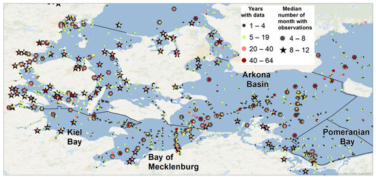
Figure 1.
The south-western Baltic Sea and the four analysed assessment units: Kiel Bay, Bay of Mecklenburg, Arkona Basin and Pomeranian Bay. The color of the dots indicates the number of years with available observations. Stations with more than 20 years of data are highlighted as hexagons, if observations from at least 4 months every year are available, or as stars if observations are available for 8 or more months.
2.1. Data Preparation
To be able to estimate areas below the critical oxygen thresholds for each year, the annual minimum near-bottom oxygen concentrations (NBO) of each station were derived from all available observations. Therefore, we gathered the available data from several freely usable sources: the IOW measurement database [44], ICES Dataset of Hydrography [45], Boknis Eck time series [46], EU Copernicus Marine Data Store [47], and the databases of the Mecklenburg Western Pomerania state office for Environment, Conservation and Geology (LUNG-MV) and the Schleswig-Holstein state office for the Environment (LfU-SH, formerly LLUR-SH), respectively. From these different databases, we extracted the measured dissolved oxygen concentrations (or the measured oxygen saturation, which was converted following Weiss [48]), location (longitude, latitude, water depth), and the depth of measurement. Aiming to unify the data in the joint dataset, the different datasets were transformed to mg/L, duplicates were removed, and measurements at the same time and location obtained by different methods were averaged. Due to many inconsistencies between the measurement depth and bathymetric depth as well as large variations in the measured bathymetric depth of the respective measuring stations, the measured bathymetric depth given in the datasets was replaced by the bathymetric depth retrieved from [49,50]. These datasets mentioned above included measurements of dissolved oxygen from the whole water column. To sort out the NBO, the deepest measurement was used, and if it was close enough to the bottom, it was used as the threshold; for water depths below 16 m, measurements within the lower 25% of the water column and water depths above 16 m measurements from a maximum of 4 m above the sea floor were selected.
2.2. Geostatistical Methods
To gain a suitable input dataset for the geostatistical methods, the above-described dataset [51] was further prepared. Firstly, data entries with measurements of NBO with more than 15 mg/L were removed, as such high values corresponded to oxygen saturation levels above 150%, while we wanted to focus on oxygen deficiency situations. Then, measurements in close proximity (1 km radius) were combined into one measuring station, and only stations that were probed multiple times were kept in the dataset. Aiming to eliminate non-plausible entries, for each station, outliers were removed and were defined as values above or below the mean +/− 3×std. Finally, the lowest NBO of each measuring station within the critical months of July to November for each year was selected. Observations from the other months were not considered as usually high NBO occurred, which could falsify the estimated areas of the annual minimum situations. Based on the derived annual minimum NBO for each station, we applied different geostatistical methods to estimate NBO everywhere in the western Baltic Sea. Therefore, two spatial interpolation methods (IPDW and Kriging) were applied, where the estimate was solely based on the measurements, as well as the machine learning algorithm Quantile Regression Forest; this additionally used a set of predictor variables for the input. All methods were applied to estimate NBO on the same raster with grid cell lengths of approx. 1 nm given by the input parameters of the Quantile Regression Forest.
In order to calibrate and test the different geostatistical methods, the year 2015 was selected as it is within the years used for the latest “State of the Baltic Sea” Holistic Assessment HOLAS-II [23,24] and had a good coverage of the measurements.
2.2.1. IPDW (Inverse Path Distance Weighting)
First, a modified Inverse Distance Weighting method was applied [52], as implemented in R [53]. This straightforward approach estimated the value of any raster cell as a weighted linear combination of the sampling point values. The weighting of the sampling point values was based on the (normally Euclidian) inverse distance to the sought point. The weighting of closer points over more distant ones was adjusted by raising the inverse distance to the power p. The Inverse Distance Power (p), in addition to the maximal distance (d), was, thereby, optimised for the test year 2015, using a Leave One Out Cross Validation. To take into account the coastline acting as a barrier, IPDW used the distance over water instead of Euclidian distances.
2.2.2. Ordinary Kriging
Kriging is a well-established spatial interpolation technique [54], which has also been applied particularly in coastal areas, e.g., [55], despite its theoretical assumptions, which are often difficult to meet in practice, e.g., as stationarity is assumed [56]. In contrast to IPDW, Kriging is a non-convex method, and not only the distance but also the spatial autocorrelation structure is included in the estimation. For this study, the Ordinary Kriging method was applied, as it provided similar interpolation estimates compared to the Universal Kriging method (which has less strict assumptions regarding stationarity), though Ordinary Kriging is easier to use [29]. Similar to IPDW, the estimated value is a weighted average of the sampling points, whereas the weights were calculated by minimising the mean squared prediction error under the constraint of unbiasedness. Thus Ordinary Kriging is often referred to as the best unbiased linear estimator [57]. The spatial autocorrelation structure, which was here assumed to be stationary and, thus, only dependent on the distance over water between two locations, and represented by the semi-variogram, was estimated based on the observational data of each year. Despite being computationally efficient, computing the semi-variogram required a lot of time to ensure the best fit for the observations for each year; this would not have been the case if using a single semi-variogram for all years. Subsequently, a theoretical parametric model was fitted to the experimental semi-variogram on which the weights were then calculated. After normalising the oxygen measurements with a box-cox transformation, a suitable model and initial values for the model parameters were selected based on the model performance parameters RMSE and R2, which were obtained from Leave One Out Cross Validation. To achieve this, the geoR package (version 1.9-2) [58] as well as the extension GeoRcb (version 1.7-7) [59,60] were used, which allowed the admission of custom distance matrices. Contrary to the IDPW method, the validity of this method could not be upheld if non-Euclidian were used [61]. We, therefore, transformed the water distance matrix to a similar Euclidian matrix via multidimensional scaling [62,63].
2.2.3. Quantile Regression Forest
The Quantile Regression Forest (QRF) algorithm is a generalisation of the Random Forest Algorithm [64], which was developed by Breiman [65] and has already been successfully applied in spatial predictions [31]. QRF allows (other than the classical Random Forest) the estimation of prediction uncertainty [31], as the spread of response variables is considered [64], allowing us to calculate the standard deviations and express the response variable’s range for each location and year. As QRF is a tree-based algorithm, decision trees were constructed based on 1000 bootstrap samples of the input data [66]. At each node, the predictor, which partitioned the data best, was selected from a random subset of (predictor) variables [67]. This random selection of predictor variables ensured a reduction in the correlation among trees. For the final estimate, individual trees were averaged. As machine learning methods are prone to overfitting, especially when data are autocorrelated [68], many validation strategies like k-fold Cross-Validation lead to an overestimation of the model performance. This autocorrelation occurs especially when working with spatial data. In order to avoid this, we followed the method proposed by Meyer and Reudenbach [68], implemented in the R package CAST (version 0.7.1) [67]. This allowed us to apply a target-oriented Leave Location Out Cross-Validation (allowing a more realistic estimate of the model performance to be provided) and forward feature selection (FFS), which might improve the model selection [66]. To test its added value, QRF with and without FFS was applied.
For the presented case study, we used only physical parameters (like near-bottom water temperature and salinity) as the input for the QRF, which had a direct effect on the solubility of NBO. As intense and stable stratification leads to oxygen deficiency below the pycnocline [69], additional input parameters were addressed the thickness of the water layer above and below the pycnocline, as well as the density difference between the surface and bottom water. All these predictor variables were extracted from a long-term model simulation with a well-established hydrodynamic model system [70]. In addition, bathymetric depth was also included asa predictor. To account for this annual variability, we trained a new QRF model for each year based on data for that particular year. Following Meyer and Pebesma [71], we further computed the area of applicability (AOA) based on the dissimilarity index compared to the training data. AOA then resulted in a binary value for every raster cell with values 0 and 1. This later value indicated that QRF was able to learn about relationships based on the training data and the estimated cross-validation performance held.
3. Results
3.1. The Joint Dataset
Gathering all the available monitoring data allowed us to gain an impressive dataset with 145,610 entries; these were used as the input for geostatistical methods later. Nevertheless, gathered data on their own already allowed some conclusions to be considered before analyzing the areas below critical thresholds. In Figure 1, stations with the longest available time series were highlighted, although strong differences regarding the number of years with available data for each station were remarkable, as well as the mean number of months with observations., e.g., IOW´s long-term monitoring stations provided for up to 65 years of data, but were monitored usually less than six months each year, resulting in a high risk that the annual minima often did not observe. On the other hand, many near-coastal stations were integrated into monitoring over the past few decades and were visited more often (mostly once per month). Their time series with available observations covered fewer years but were mostly still more than 20 years (see Figure 1). Several automatic measuring stations (like Oderbank) were included in the joint dataset, which provided data at a high temporal resolution, resulting, e.g., in Pomeranian Bay in a high number of observations per year for the HOLAS-II assessment period, while the number of available stations was low (see Figure S1 in the supplement).
The pure number of available observations increased steadily from 1950 up to 2005, when approx. 2000 data points were available in the four assessment units (see Figure 2a). The number of sampled stations was highest around 1995 (especially in Pomeranian Bay; Figure 2b) but remained stable with approx. 150 to 200 annual stations afterward, while the pure number of available observations has decreased since 2005 (see Figure 2a).
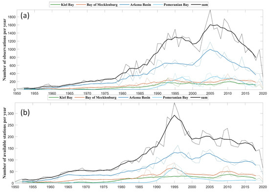
Figure 2.
Number of observations (a) and number of available stations (b) per year for each assessment unit in the western Baltic Sea, where bold lines are the 5-year running means.
First, measurements of NBO below 2 mg/L were traced back to 1953 in Kiel Bay, 1958 in the Bay of Mecklenburg, and 1960 in the Arkona Basin—indicating that small-scale and local hypoxic events have occurred in the western Baltic Sea (except Pomeranian Bay) at least since the middle of the 20th century. NBO followed a strong seasonal cycle, which was quite comparable in all four assessment units (see Figure 3a), with the highest values in winter and spring and the lowest values between June/ July and October. Pomeranian Bay had mostly higher values of NBO, indicating that hypoxia might be less critical than in other assessment units. The standard deviation of monthly values was quite high (up to 3.5 mg/L), but it was thereby dominated by a strong variability within the assessment units, while interannual variability was weaker (see Figure 3b). The unit-wide mean values for a multi-year assessment period (like HOLAS-II) depended strongly on the order of computing steps, i.e., if first the spatial averages were calculated and then the temporal ones, or vice versa (see Figure 3b).
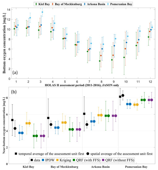
Figure 3.
(a) Climatology of the near–bottom oxygen concentrations [mg/L] averaged from the available stations in the complete assessment units [43] from the HOLAS-II period (2011–2016); (b) The mean values (July to November values only) for the assessment units of HOLAS–II periods computed by first calculating the spatial average and afterward the temporal average (squares) or vice versa (dots) based purely on the observations (black) or after closing the gaps with different geostatistical methods.
3.2. Comparison of the Different Geostatistical Methods for One Test Year (2015) and the HOLAS-II Assessment Period
Since IPDW is a parametric method, suitable values for the model parameters Inverse Distance Power (p) and Maximal Distance (d) had to be selected. Based on these two model performance parameters, RMSE and R2, which were obtained from a Leave One Out Cross Validation, the best pair was identified with d = 45,500 and p = 0.5 (see Table 1); these were then also used for other years. Compared to the other applied methods, Kriging had the highest RMSE and lowest correlation coefficient (see Table 2). Both Quantile Regression Forest (QRF) approaches gained better results, whereby performing forward feature selection (FFS) was beneficial. All geostatistical methods overestimated the very low NBO concentrations and also underestimated the high NBO of above 6 mg/L (see Figure 4), whereby the bias was lower for QRF. Nevertheless, in all methods, single data points could be identified, which differed very strongly, e.g., both QRF variants estimated very low NBO concentrations of around 1 mg/L, while 9.5 mg/L was observed. Testing a variety of different combinations for the input variables revealed that the best QRF model with FFS of 2015 was achieved with three input variables; these were even slightly better than adding a fourth input variable (see Figure 5a). Thereby bottom salinity and bottom temperature had the highest importance for the best QRF model, while mixed layer depth had only a very minor influence (see Figure 5a). For both QRF methods, their applicability was very high, as indicated by AOA equal 1 for at least 98.5% of the different assessment units.

Table 1.
R2 and RMSE for IPDW for the year 2015 computed with selected values of maximal distance (d) and Inverse Distance Power (p), with the best parameter pair in bold.
Table 2.
RMSE and R2 of the case study year (2015) for the applied methods (the number of observations = 296, mean of observations = 4.37 mg/L).
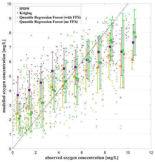
Figure 4.
Comparison of the observed and model near-bottom oxygen concentrations in 2015 from the different geostatistical methods. Dots show the single measurements; squares show the means and standard deviations within ranges 0–1, 1–2, …
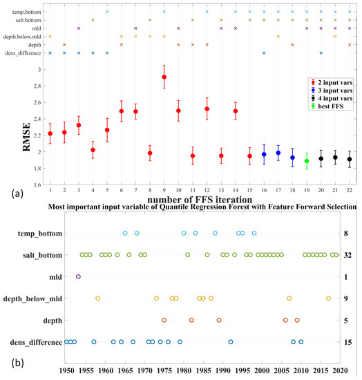
Figure 5.
(a) The feature forward selection took 22 steps and gained the best QRF model (with FFS) for 2015 using bottom salinity and temperature, as well as mixed layer depth (mld); the iterative process started by testing all combinations of the two input variables (red circles). After finding the best pair, a third input variable was added (blue circles) and finally four input variables were tested (black circles); however, RMSE worsened compared to the best combination with 3 input variables (green circle); (b) The most important input variable of the QRF model with FFS for each year. The right numbers are the total quantities of each input variable over the whole time series. dens_difference is the density difference between the surface and bottom.
Following the latest HELCOM assessment (HOLAS-II), we estimated the annual minimum of NBO with different geostatistical methods and computed the spatial extent of the regions with NBO below critical thresholds for the HOLAS-II period as well (2011–2016). The data coverage of the input stations ranged widely (Figure S1). For eight stations in Kiel Bay, measurements were available for all six years, as well as twelve stations in the Bay of Mecklenburg, 24 stations in Arkona Basin and seven stations in Pomeranian Bay. But there were also a couple of stations where only one year was usable (see Figure 6). Already from the means of the annual minima from station data, some hotspots with a very low NBO could be detected, e.g., in the southern Bay of Mecklenburg or the western Kiel Bay.
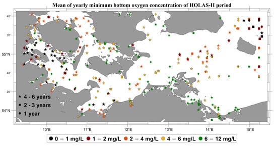
Figure 6.
Mean of the yearly minima of near-bottom oxygen concentrations [mg/L] evaluated for the HOLAS–II period (2011–2016) using only data from the critical period (July to November). Different oxygen concentrations are colour coded; the different symbols indicate how many years were available for each station.
Both interpolation methods tended to produce maps in which the very low NBO (especially below 1 mg/L and also below 2 mg/L) were hardly visible (see Figure 7), coinciding with the results from 2015 (see Figure 4). While the single stations with NBO below 1 mg/L were still recognizable in the Kriging map (see Figure 7b), they seemed to vanish completely at IPDW (see Figure 7a). This was less the case FOR QRF, as both variants reproduced NBO minimum areas, which STOOD out already from the point data (see Figure 6). Following the area of applicability method (AOA), the uncertainty of the spatial prediction could be estimated at QRF (see Figure S4). Both variants had an AOA value of one for nearly the whole region during the HOLAS-II period (see Figure S2a,b), indicating that the training data allowed QRF to be applied almost everywhere. The mean standard deviations of the QRF results, reflecting the internal range width of the estimated NBO, had a remarkable gradient with the largest values in Kiel Bay and the Bay of Mecklenburg (see Figure S2c,d).
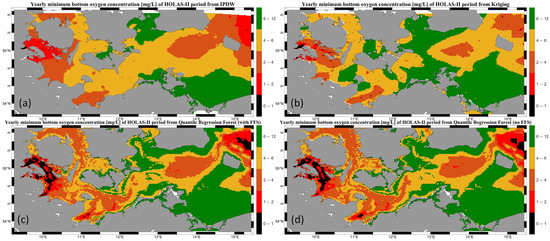
Figure 7.
Mean annual minimum for the HOLAS–II period (2011–2016) of the bottom oxygen concentration [mg/L] using different geostatistical methods (a) IPDW; (b) Kriging; (c) Quantile Regression Forest with FFS; (d) Quantile Regression Forest without FFS).
Other than for pure observational data, the mean values of the HOLAS-II period for each assessment unit depended no longer on the order of computing spatial and temporal averages after NBO was estimated for the full areas (see Figure 3b). The areas with high interannual variability (expressed through high standard deviations; see Figure S3) differed quite strongly between these methods. At QRF, the regions with highly dynamic currents, like the edges of the deeper part of the Arkona Basin, also had the highest interannual variability. In the interpolation methods, the standard deviations from the six-year period were quite high around the regular monitoring stations and in parts where NBO was quite high in single years, such as the north-western Bay of Mecklenburg.
The share of areas below the critical thresholds was much lower for IPDW and Kriging than for QRF (see Figure 8). At IPDW, the hypoxic regions were 5.4% above Kriging (1.1%) in Kiel Bay and 2.8% (IPDW) resp. 2.4% (Kriging) in the Bay of Mecklenburg. These estimates were clearly below the ones from QRF, which were 25 to 30% for Kiel Bay and 18 to 20% for the Bay of Mecklenburg. Despite these single differences, at all methods, the region with very low NBO was larger in Kiel Bay and the Bay of Mecklenburg, while in Pomeranian Bay, only a small share of the area had an NBO between 4 and 6 mg/L. Arkona Basin ranged in the middle compared to the other assessment units but still had approx. 10% of the area with NBO below 2 mg/L at QRF. This regional coherence was quite high, and, as in all geostatistical methods, the same areas had an NBO strongly below the assessment units’ mean (see Figure S5).
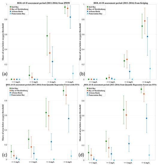
Figure 8.
Share of areas with NBO below the threshold for each assessment unit using different geostatistical methods (a) IPDW; (b) Kriging; (c) Quantile Regression Forest with FFS; (d) Quantile Regression Forest without FFS).
3.3. Temporal Analysis for the Different Assessment Units
In Figure 9, the decadal means of pure number for observations in each assessment unit are shown together with the share of areas below critical threshold concentrations. In all four assessment units, the number of observations was very low for the first decades, whereas a minimal number was mostly reached in the 1960s. An exception was Arkona Basin, in which the number of observations increased steadily until the last decade.
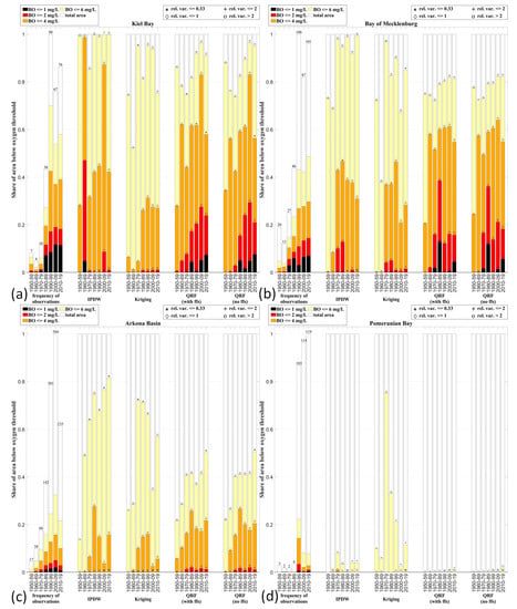
Figure 9.
Temporal development of the area shares below the different bottom oxygen concentration thresholds for each assessment unit (a) Kiel Bay; (b) Bay of Mecklenburg; (c) Arkona Basin; (d) Pomeranian Bay) using the different geostatistical methods. The symbols indicate the relative variance, calculated as the standard deviation per decade divided by the mean. The first set of bars indicate the mean number of used observations per year for the different decades.
As already seen for the test year, the interpolation methods had a higher RMSE than the two QRF variants (see Figure S4). Nevertheless, at least over 11 (4) years, IPDW (Kriging) resulted in the lowest RMSE of all four methods. QRF with FFS was the best method over 42 years, while QRF without FFS gained the lowest RMSE for 13 years. On average, performing feature forward selection reduced the annual RMSE by 3.5%, while IPDW (Kriging) had an approx. 8.6% (23.0%) higher annual RMSE compared to QRF with FFS. FFS gained the best model mostly with only four of the six input variables (in 25 years; 35.7%), while in 16 years (22.9%) and 15 years (21.4%), three or five input variables led to the best models. In nine years (12.9%), only two variables were best, and in five years (7.1%), using all six variables was best. Thereby, each input variable was identified as the most important for each year’s best model for at least one time (see Figure 5b). The bottom salinity was ranked as the most important input variable in 32 years (45.7%), followed by the density difference between the bottom and surface (15 years, 21.4%), the water volume below the mixed layer depth (9 years, 12.9%) and the bottom temperature (8 years, 11.4%).
For both QRF models, areas of applicability (AOA) were computed (see Figure S7a,b). In Arkona Basin, both methods had a high degree of trustworthiness in their deeper parts, while it was low in shallower parts. The AOA was also high in large parts of Kiel Bay and the Bay of Mecklenburg, especially without FFS. At once, QRF without FFS seemed less applicable in the Pomeranian Bay (see Figure S7b). The share of areas with AOA equal to one was thereby mostly increased over time, indicating that the reliability of QRF models was higher in later years (see Figure S7c). Only a low pure number of observations indicated that they had an influence on the extent of the trustworthy region (see Figure S7d). As soon as the number of observations was approx. above 15% of the maximal available observations for one year, the trustworthy region was not affected anymore.
Both interpolation methods estimated (similar to the HOLAS-II assessment period) only very small areas with very low NBO during the whole time period. One exception was the 1960s in Kiel Bay, where only a very low number of observations was available, resulting in a very large extent of the area with less than 1 mg/L at IPDW. This peak with a high area share was not visible in Kriging at all; instead, it was the decade with the smallest area there. Both QRF models showed a steady increase in the areas with low NBO until the start of the 21st century before they partly dropped during the last decade (see Table 3).
Table 3.
Share of stations and areas using the different geostatistical methods of this study compared to the reanalysis study of Kõuts, Maljutenko [72] and the model study by Piehl, Friedland [25] for selected critical thresholds in the different assessment units. Please be aware that Kõuts, Maljutenko [72] only provided results from 1993 on.
Observations with NBO below 2 mg/L were in Kiel Bay already quite often in the 1950s and 1960s increased from approx. 10% of stations to 25% in 2000–09 and 21.1% after 2010 (see Table 3). The rise in hypoxic stations was well reflected by hypoxic areas from the QRF models, which showed an increase in hypoxic areas from 0 to 5% in the first decades up to nearly 30% after 2000. In the last decade, the share of hypoxic areas decreased slightly from 21.1 to 23.9%, while the interpolation methods estimated that only 1% of Kiel Bay was hypoxic (see Table 3).
The increase in hypoxia was even more drastic in the Bay of Mecklenburg, where only 1.2 and 3.1% of the stations were hypoxic during the first decades, while after 2000, it was 15 to 16.3%. The rise in hypoxic stations was again reflected by the hypoxic areas from the QRF models, which showed an increase in the hypoxic areas from 0 to 2% in during the first decades to 15.7–18.2% in the last decade (see Table 3). In the Bay of Mecklenburg, the maximal extent of the hypoxic area was reached in the 1980s, when more than one-third was hypoxic in both QRF models (see Table 3). Like Kiel Bay, both interpolation methods provided very low shares of the hypoxic areas in recent decades, while their maximum was also reached in the 1980s, like that estimated by the QRF models.
For Pomeranian Bay, only NBO below 6 mg/L was relevant. While the decadal variability of the station share was very high, both QRF models estimated only very low area shares with less than 2% over the last decade. The shares increased slightly for the last two to three decades in QRF models while, beforehand, both estimated that none of the areas had an NBO below 6 mg/L. This is not in line with the observations, as up to 25% of the stations had NBO below 6 mg/L. While IPDW estimated a slightly larger area share of up to 8% in the 1970s, the areas estimated by Kriging were substantially larger (with a maximal value of 75%, see Table 3). The areas from interpolation methods were also partly influenced by stations from the surrounding assessment areas, as often, no suitable station was located in the northern and eastern parts of Pomeranian Bay. For the first decade, Kriging estimated that 10% of the area had an NBO below 6 mg/L, although no station with less than 6 mg/L was found in Pomeranian Bay, indicating that this low NBO was induced by stations outside of Pomeranian Bay.
3.4. Training QRF with Data from 2015 and Applying It to the Whole Time Series
One advantage of QRF is that it allows model scenarios to be run, asking “what if” questions. To exploit this, we trained the QRF models purely with the observational data from 2015, when AOA had the highest values, and applied them afterward to the full-time series. These derived results allowed us to assess if the change in hydrodynamic conditions over the past few decades relating to stratification had an impact on the hypoxic areas on top of human-induced pressures, which were reflected by the NBO measurements of 2015.
The resulting decadal means of the areas below the different thresholds are shown in Figure 10. This scenario resulted in all assessment units except Pomeranian Bay in areas with a low NBO to be larger than in the original QRF model runs that were trained individually for every year. The steady increase in the areas over the decades was less pronounced in this scenario, especially the area with an NBO below 4 mg/L, which only slightly fluctuated. Further, the three decades at the end of the 20th century often had the highest area share with a very low NBO, indicating that the hydrodynamic conditions caused a worsening of the hypoxic situation during the stagnation period in the 1980s and 1990s. This was broken up after 2000, when the areas below the critical thresholds were nearly on the same level as in the 1950s and 1960s, indicating that the hydrodynamic conditions had a comparable effect on oxygen deficiency between different decades. Training the QRF models with the data of 2015, a year when many stations had a low NBO, led to Kiel Bay having much higher shares in the areas below 2 and 4 mg/L compared to individually trained QRF model runs. On the other hand, Arkona Basin and Pomeranian Bay had, after the strong Major Baltic Inflow of 2015, nearly no stations with a very low NBO. In Pomeranian Bay, this resulted in NBO never appearing below 6 mg/L in the scenario during the whole time series. Due to the restriction of the training data to only one year, the areas of applicability decreased by approx. 9.5% (QRF with FFS) and even 15.4% (QRF without FFS). Overall, the differences between the runs with and without FFS were stronger in the scenario than before, although the area shares for 2015 were quite the same.
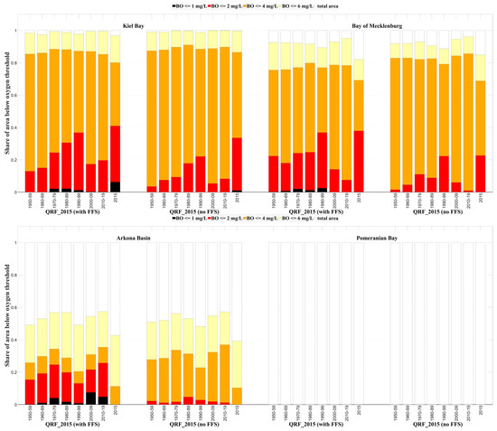
Figure 10.
Temporal development of area shares below the thresholds for each assessment unit from the two QRF variants, trained only with observations from 2015.
4. Discussion
4.1. The Joint Dataset
Dissolved oxygen is essential for all marine life, especially for benthic organisms that live on the seafloor without being able to escape if oxygen concentrations fall below critical thresholds [20]. Therefore, near-bottom oxygen concentrations (NBO) and the spatial extent of areas with low NBO are key components of environmental assessments like HOLAS [23,24] and legislations, like the EU MSFD [6]. Due to its importance, NBO is measured widely by authorities, environmental agencies and researchers in the western Baltic Sea (see Figure 1). Unfortunately, until today, no common database has been implemented where all quality-ensured observations are stored and freely available. Instead, several independent databases exist and are filled regularly with new data but differ with respect to their formats, units and update time steps. To overcome this problem, several local and global initiatives have been launched, e.g., GO2DAT [73], by the World Resources Institute [74] or within the Copernicus programme [47]. Nevertheless, until now, data were spread in different databases and had to be combined individually to gain a consistent dataset (see Figure 1). Performing this step repeatedly for single studies, e.g., [7,11,75], does not seem very sustainable and is unnecessary work. Instead, a consistent, permanently updated and freely available database is needed where all quality-controlled measurements are gathered and made publicly available [51].
Using the available data [44,45,46,47] and the databases of local environmental agencies (LUNG-MV and LfU-SH), were able to gather oxygen data from the whole western Baltic Sea. This compiled dataset included nearly 150,000 entries and proceeded back to the beginning of the 20th century. Single observations could mostly be allocated to individual stations, which differed substantially, e.g., with respect to the number of years with available data or the number of measurements per year, resulting in strong differences in the spatial coverage of assessment units in the western Baltic Sea (see Figure 6 and Figure 8). While temporal and highly resolved stations (e.g., from the MARNET monitoring network [76]) allow short-term oxygen dynamics to be analysed, others have a lower high temporal resolution but have been monitored over six decades (e.g., along the Baltic Thalweg [22]) allowing the study of the long-term development of oxygen deficiency situations. Bringing together these different stations in a consistent way is challenging but necessary to derive the extent of areas with NBO below critical threshold concentrations.
4.2. Potentials, Strengths and Weaknesses of the Geostatistical Methods Assessing the Critical Areas
As it was one of our key aims to close spatial gaps and to obtain from the point data the full picture, we needed a suitable (geostatistical) method to estimate NBO, where it had not been measured. Specifying a priori which method is best or even which should be tested is a challenging task. Based on previous approaches, we decided to apply IPDW (Inverse Path Distance Weighting) and Ordinary Kriging as interpolation methods, as both have already been used to estimate the hypoxic area in the central Baltic Sea, e.g., [75,77]. On the other hand, machine learning techniques may overcome most shortcomings of interpolation methods and are, therefore, increasingly applied to estimate hypoxic areas [34,37,78]. Out of the variety of potentially usable ML approaches, we selected the Quantile Regression Forest (QRF) with and without feature forward selection (FFS). It has already been successfully used to predict spatial fields and allow for the estimation of prediction uncertainty [31].
It is hardly possible to judge which geostatistical method is the best to estimate the annual extent of the area with NBO below different critical thresholds because no reliable product is available yet which could be used as a benchmark. Instead, only the fit of estimated NBO concentrations with measured ones could be compared (see Figure 4 and Table 2; Figure S6), showing that RMSE and correlation were worse for interpolation methods compared to both QRF variants. Validating the derived annual NBO fields from the present state (Figure 4) seems only possible by comparing them to reanalysis results [72] or purely model-based estimates, e.g., [25]. While reanalysis agrees more with the results from interpolation methods (see Table 3), the biogeochemical model fits better with the area shares estimated by QRF. Nevertheless, all four geostatistical methods, as well as Kõuts, Maljutenko [72] and Piehl, Friedland [25], identified the same regions with the strongest oxygen deficiency (see Figure S5) and also showed a slight improvement in the oxygen deficiency situation in the western Baltic Sea over the last three decades (see Table 3). However, comparisons are complicated, as the reanalysis, as well as the model results, allow critical areas to be estimated at least at a monthly resolution. With our approach to computing first the annual mean of each station before filling the spatial gaps, only annual estimates were gained. Further, the proceeding might lead to an overestimation of areas with low NBO if the annual minima do not occur at the same time. To overcome this shortcoming more temporal highly resolved data are needed so that data-driven methods may also consider temporal development during the year. Further, performing a 1:1-comparison of data vs. model points works well for QRF models, while the applied LOOCV for the interpolation methods means that one point is not used for the IPDW or Kriging, as this point is needed to compute the model quality. This means that the best result was not used in both interpolation methods, as it was to be assumed that the model with the extracted data point would be better without it. At once, only by taking out every point RMSE and correlation coefficient could they be computed.
Applying QRF with feature forward selection (FFS), the near-bottom salinity was identified as the most important predictor (see Figure 5b). In most years, only three of the six available input parameters were needed for the best FFS model, indicating the strong overlap between different input variables. Adding more factors, as suggested by Schourup-Kristensen and Larsen [9], which are independent of already-included ones (like biomass production, sediment type, carbon content in the sediment or bioturbation), might improve the QRF quality further. To include these additional parameters in the QRF model, reliable estimates are needed for the period of interest (1950–2019 in our case). Since no suitable observations for the whole time were available, only the output from a biogeochemical model seemed usable. In order to compare the results of the geostatistical model with ERGOM-MOM [25] (e.g., Table 3), we, therefore, only included parameters that were constant over time (like bathymetric depth) and addressed only hydrodynamic features.
Despite gaining gap-free spatial fields (at least for most years), both interpolation methods had their individual shortcomings. Both assumed the general continuity of the region, resulting in the point that equidistant observations obtained the same weight without considering natural gradients. Although two-dimensional maps are generated by selecting only the bottom-closest observations, the oxygen concentrations can be seen more as three-dimensional fields. They depend on the location as well as the bathymetric depth and measurement depth. This is hardly considered by the used interpolation methods, although—in theory—this has already been improved by the Kriging method, which estimates the spatial autocorrelation from the data. It is expected that this is a better way to combine the observational data than the pure distance between them [29,62]; however, for our dataset, Ordinary Kriging was the worst of the used geostatistical methods (see Table 2; Figure S6). Further, both interpolation methods encountered the problem that Euclidean distances were insufficient for interpolation in coastal areas. Replacing the Euclidean distances simply by the water distances violated the validity of the Kriging method [61]. Instead, we use multidimensional scaling to transform the water distance matrix into a similar Euclidean matrix [62,63] since it can be easily implemented in R. More advanced Kriging approaches, like Regression Kriging [79], could gain better results. There are also Kriging variants with alternative ways of calculating the non-Euclidian distances [27,80], which allow us to consider more information (e.g., auxiliary variables comparable to the input parameters of the QRF) while having less strict a priori assumptions [81]. In particular, fitting the experimental semi-variogram to obtain suitable weights based on the observations of each year is challenging, time-consuming, requires high accuracy and can falsify the results. Selecting a priori, the specific IPDW parameters was hampered due to the high computational effort; therefore, only a finite number of parameter pairs could be tested, resulting in a good but not optimised parameter pair.
QRF is easily automatable; therefore, running it for all years with the available data is much faster than for the interpolation methods. It also has the advantage that less a priori work (like computing the semi-variograms or finding optimal parameters) or specific assumptions are necessary. It is only necessary to choose and find suitable input parameters that cover the area and time span of interest. QRF even allows highly correlated input variables to be included, like depth, mixed layer depth and depth below the mixed layer in our case. On the other hand, QRF is some sort of black box as the user cannot simply verify the rules or how the NBO concentration at a specific time and place is determined. This makes analysing the output maps comparably intricate, as it can hardly reconstruct why the algorithm estimates a certain value; therefore, that identifying artifacts is more demanding compared to the interpolation methods. Further, QRF can hardly reproduce every data point (what the interpolation methods do automatically) and might even be at risk for the overfitting of data [82].
One obstacle in our case included contradicting observations near each other. This hurdle is only a minor issue for QRF, while the interpolation methods stumbled. The problem may become dampened by weighing the observations if it is possible to judge which data point is more trustworthy without falsifying the assessment. This problem plays less of a role in the QRF variants, which do not reproduce every data point precisely but use more information to generate a sophisticated estimate. Furthermore, IPDW as a conex interpolation method suffers from the shortcoming that it cannot estimate NBO values lower (or higher) than the input data. This holds not for Kriging (which is a linear method as well as non-convex) nor for QRF. Indeed, Kriging estimates for 20 years produced a lower annual minimum NBO overall observation stations than it was observed, while both QRF variants estimated NBO only within the range of the measurement station. QRF can also be applied to values of the input variables outside of the range provided by the training data [83], but this may result in less reliable estimates, visible by the low area of applicability (AOA) values (see Figure S7), following [71]). Being able to identify regions where prediction might become less reliable is a strong advantage of QRF (Figures S3 and S4 in the Supplementary Material); additionally, Kriging may offer comparable uncertainty estimates. Finding and selecting training data in a way that AOA can become maximised is a key challenge to all machine learning approaches [31]. In our case, already 15% of the maximal available observations for one year were needed to gain high AOA values. Increasing the pure number of used data points had no added value (see Figure S7b), indicating that the position of the data points was also essential to gain a meaningful and representative training dataset. Applying QRF every year individually was a good way to obtain the interannual variability as the interpolation methods did; however, it narrowed down the training dataset drastically. Aiming to provide widely spread input and training data might have led to a disproportionate representation of higher NBO measurements in our case. Without restricting the training data a priori, too many data points with high NBO may have been included so that the few points with a low NBO were superimposed, leading to a potential underestimation of the areas below the critical oxygen threshold concentrations at QRF. Focussing the training dataset on points with a very low NBO (e.g., by introducing special weights) without losing the bandwidth of real-world observations is a complicated trade-off but might allow the results to be improved in the future by tailoring methods that are better to specific oxygen deficiency situations.
Despite these individual strengths and weaknesses, all applied geostatistical methods had their individual problems when estimating the NBO in Pomeranian Bay. The interpolation methods come to the edge of their areas of trust, as most of the regular monitoring stations are located in the southwestern part of Pomeranian Bay, while in many years, nearly no data were available in the northern and eastern parts. This problem was especially visible in the 1950s, when no station had an NBO below 6 mg/L, while Kriging estimated that 10% of the area was below 6 mg/L. This was induced by stations outside Pomeranian Bay, which could affect the interpolation accordingly. On the other hand, both QRF variants seem to underestimate the areas with low NBO. This can be induced by a bias within the training data, as fewer stations are located in Pomeranian Bay compared to the other assessment units (see Figure 2). As the background conditions are different in Pomeranian Bay, which is characterised by sandy sediments and high pelagic primary production [84], the machine learning algorithm might fail to adjust to this special region, as these factors are not incorporated as input parameters. This problem may be bypassed by developing subscale QRF models for the single assessment units and bordering areas.
4.3. Assessing the Pre-Eutrophic State and the Temporal Development since It
After evaluating the different geostatistical methods to the test cases, they were applied to all years with data available. This allowed the development of hypoxic areas to be traced since 1950, which is regarded as a time when eutrophication pressure was still low and the western Baltic Sea ecosystem was still in a good environmental state [38,39]. Both the coupled biogeochemical model applied by Piehl and Friedland [25], as well as our results show that hypoxic events occurred in the early 1950s and 1960s. This probably occurred even more often than the observations showed, as only a few measurements were available from that time (see Table 3). This oxygen stress was amplified by eutrophication and a changing climate, resulting in drastically increasing hypoxic areas.
Following Skogen, Ji [42], hereafter, the model results of Piehl and Friedland [25], and our observation-based ones are integrated to estimate the pre-eutrophic state. To streamline the analysis, only one critical NBO threshold was selected for each assessment unit. Considering the range of the areas below 2 mg/L in Kiel Bay, which were between 0 and 4.9% in the present study, the value estimated by Piehl and Friedland [25] could serve as a realistic estimate for the undisturbed state, which was with 2% (for 1960–1969) the middle of the geostatistical methods. In the Bay of Mecklenburg, our estimates were with values between 0 and 2%, substantially lower than Piehl and Friedland [25], who estimated up to 16.4% of the area to be below 2 mg/L in the earliest decades. As the assessment unit seems quite comparable to Kiel Bay with respect to the hydrodynamic features, as well as the number of stations and the area shares below the different critical thresholds (see Table 3), an extent of the hypoxic area at 2% might be reasonable for the pre-eutrophic state. In both assessment units, reaching such low hypoxic areas is very ambitious given present-day eutrophication pressure. In Figure 10, which critical areas that occurred when the QRF variants were trained with the observations of 2015 (representing the highly eutrophied state) are shown when applied to the hydrodynamic conditions from 1950 onwards. The results indicate that the hypoxic areas stayed even in the decades with the best hydrodynamic conditions, mostly above 10%, so the pre-eutrophic estimates of 2% were only reached if the eutrophication pressure was strongly reduced. At once, using only one year of observations instead of the total led to an under-learning effect of the QRF variants, visible in clearly reduced AOA values.
For Arkona Basin, already 4 mg/L seems a critical oxygen concentration (see Figure 3, Figure 7, Figure 8 and Figure 9), while the interpolation methods provide hardly lower NBO (see Figure 9). Therefore, 4 mg/L is depicted here as a critical threshold. The areal estimates were between 0 and 10.3% for the pre-eutrophic state in the geostatistical models, while Piehl, Friedland [25] seemed to be quite in the middle with 4.6% for the period 1960–69. This value might be a realistic estimate for the pre-eutrophic situation, but it is still quite challenging to achieve it with eutrophication pressure nowadays (see Figure 10). In Pomeranian Bay, where the oxygen situation overall is less critical, NBO concentrations below 6 mg/L can be seen as a warning signal, while lower NBO concentrations occur not without external disturbances. While Piehl, Friedland [25] estimated area shares of approx. 2%, our interpolation methods gained 0% for the pre-eutrophied decades, while the QRF models estimated higher area shares, although they seemed to overestimate NBO in Pomeranian Bay substantially (see Section 4.2).
For all four considered assessment units in the western Baltic Sea, comparable temporal developments of hypoxic areas occurred since the mid of the 20th century. In all units and in all geostatistical approaches, as well as in the model study of Piehl and Friedland [25], the extent of the areas below the different critical oxygen concentrations was smallest in the 1950s and 1960s. Afterward, the area extents increased, although some differences occurred when the maximum values were reached (see Figure 9 and Table 3), e.g., in the Bay of Mecklenburg and Arkona Basin, the maxima occurred mostly in the 1980s, while it was after 2000 in Kiel Bay. Afterward, a slight improvement in the oxygen deficiency situation was visible in all western Baltic Sea assessment units (see Table 3). This coincides with the trends reported by Kõuts, Maljutenko [72], and Piehl and Friedland [25] and are due to beneficial hydrodynamic conditions [85,86] and are less an expression of a reduced eutrophication pressure. This is especially true in Kiel Bay and the Bay of Mecklenburg, where the hypoxic areas were maximal in the 1990s, with eutrophication pressure comparable to nowadays (see Figure 10). The occurrence of the largest areas, with a very low NBO in the 1980s and 1990s in Arkona Basin, corresponds to Väli, Meier [87], who reported a deeper halocline for these decades, hampering the vertical mixing resulting in lower oxygen concentrations. Nevertheless, despite the decreasing nutrient inputs in the Baltic Sea [88,89,90] and more favourable hydrodynamic conditions after 2000, these hypoxic areas were substantially higher than the estimated values of the 1950s and 1960s. Reducing the areas back to their historical dimension from the pre-eutrophic state (as required by the EU-MSFD) requires substantially more effort and further nutrient input reductions.
5. Summary and Conclusions
- A comprehensive dataset with freely available observations of near-bottom oxygen concentrations covering the western Baltic Sea was compiled.
- To estimate the hypoxic area (e.g., for environmental assessments like the EU-MSFD), gap-free spatial information is needed. We, therefore, applied two interpolation methods and the machine learning algorithm Quantile Random Forest (QRF).
- Our validation results indicated that QRF combined with feature forward selection gained the best results. The interpolation methods struggled to reproduce the very low oxygen concentrations, which led to substantially smaller hypoxic areas. Further, in years with only a few observations, the same spatial gaps were not closed by the interpolation method IPDW.
- QRF has the advantage that it is easily automatable and that the uncertainty can be estimated and combined with the area of applicability, gaining more robust results.
- The hypoxic areas increased in all applied methods drastically from the 1950s to the current situation, indicating a high anthropogenic pressure. To a lesser extent, they were also impacted by the hydrodynamic conditions, especially in the 1980s and 1990s. Nevertheless, our results indicate that even in the pre-eutrophic state, hypoxia occurred in the western Baltic Sea.
Supplementary Materials
The following supporting information can be downloaded at: https://www.mdpi.com/article/10.3390/w15183235/s1, Figure S1: Number of observations and available stations per year for each assessment unit, averaged for the HOLAS-II assessment period; Figure S2: Share of years during the HOLAS-II period, when AOA was 1 at QRF, as well as the mean standard deviations from both QRF variants; Figure S3: Standard deviation of the annual minima for the HOLAS-II period (2011–2016) of the near-bottom oxygen concentration from the different geostatistical methods; Figure S4: Combination of the computed AOA and the annual standard deviations for the HOLAS-II period; Figure S5: Coherence map of the four geostatistical methods for the HOLAS-II assessment period; Figure S6: Annual RMSE of the different geostatistical methods; Figure S7 Share of years with AOA = 1; Table S1: Temporal development of the area shares below the different bottom oxygen concentration thresholds for each assessment unit from the different geostatistical methods.
Author Contributions
All authors contributed to the study conception and design. The geostatistical methods were implemented by C.V. Data were collected by all authors. The results analysis was performed by C.V. and R.F. The first draft of the manuscript was written by R.F. All authors improved the manuscript in an iterative approach. All authors have read and agreed to the published version of the manuscript.
Funding
The authors were supported by Umweltbundesamt (grant no. 3720252020, 3723252040).
Data Availability Statement
All quality-controlled measurements of near-bottom oxygen concentrations are gathered in a harmonised dataset, which has been made publicly available at [51].
Acknowledgments
Supercomputing power was provided by HLRN (North-German Supercomputing Alliance). The authors thank LUNG-MV and LfU-SH for providing all necessary data.
Conflicts of Interest
The authors declare no conflict of interest.
References
- Diaz, R.J.; Rosenberg, R. Spreading Dead Zones and Consequences for Marine Ecosystems. Science 2008, 321, 926–929. [Google Scholar] [CrossRef] [PubMed]
- Schmidtko, S.; Stramma, L.; Visbeck, M. Decline in global oceanic oxygen content during the past five decades. Nature 2017, 542, 335–339. [Google Scholar] [CrossRef] [PubMed]
- Brauko, K.M.; Cabral, A.; Costa, N.V.; Hayden, J.; Dias, C.E.P.; Leite, E.S.; Westphal, R.D.; Mueller, C.M.; Hall-Spencer, J.M.; Rodrigues, R.R.; et al. Marine Heatwaves, Sewage and Eutrophication Combine to Trigger Deoxygenation and Biodiversity Loss: A SW Atlantic Case Study. Front. Mar. Sci. 2020, 7, 590258. [Google Scholar] [CrossRef]
- Halpern, B.S.; Frazier, M.; Afflerbach, J.; Lowndes, J.S.; Micheli, F.; O’Hara, C.; Scarborough, C.; Selkoe, K.A. Recent pace of change in human impact on the world’s ocean. Sci. Rep. 2019, 9, 11609. [Google Scholar] [CrossRef] [PubMed]
- Vaquer-Sunyer, R.; Duarte, C.M. Thresholds of hypoxia for marine biodiversity. Proc. Natl. Acad. Sci. USA 2008, 105, 15452–15457. [Google Scholar] [CrossRef]
- 2008/56/EC; Directive 2008/56/EC of the European Parliament and of the Council of 17 June 2008. Establishing a Framework for Community Action in the Field of Marine Environmental Policy (Marine Strategy Framework Directive). Commission of the European Communities: Brussels, Belgium, 2008.
- Carstensen, J.; Andersen, J.H.; Gustafsson, B.G.; Conley, D.J. Deoxygenation of the Baltic Sea during the last century. Proc. Natl. Acad. Sci. USA 2014, 111, 5628–5633. [Google Scholar] [CrossRef] [PubMed]
- Breitburg, D.; Levin, L.A.; Oschlies, A.; Grégoire, M.; Chavez, F.P.; Conley, D.J.; Garçon, V.; Gilbert, D.; Gutiérrez, D.; Isensee, K.; et al. Declining oxygen in the global ocean and coastal waters. Science 2018, 359, eaam7240. [Google Scholar] [CrossRef]
- Schourup-Kristensen, V.; Larsen, J.; Maar, M. Drivers of hypoxia variability in a shallow and eutrophicated semi-enclosed fjord. Mar. Pollut. Bull. 2023, 188, 114621. [Google Scholar] [CrossRef]
- Dietze, H.; Löptien, U. Retracing hypoxia in Eckernförde Bight (Baltic Sea). Biogeosciences 2021, 18, 4243–4264. [Google Scholar] [CrossRef]
- Carstensen, J.; Conley, D.J. Baltic Sea Hypoxia Takes Many Shapes and Sizes. Limnol. Oceanogr. Bull. 2019, 28, 125–129. [Google Scholar] [CrossRef]
- Reissmann, J.H.; Burchard, H.; Feistel, R.; Hagen, E.; Lass, H.U.; Mohrholz, V.; Nausch, G.; Umlauf, L.; Wieczorek, G. Vertical mixing in the Baltic Sea and consequences for eutrophication—A review. Prog. Oceanogr. 2009, 82, 47–80. [Google Scholar] [CrossRef]
- Meier, H.E.M.; Eilola, K.; Almroth-Rosell, E.; Schimanke, S.; Kniebusch, M.; Höglund, A.; Pemberton, P.; Liu, Y.; Väli, G.; Saraiva, S. Disentangling the impact of nutrient load and climate changes on Baltic Sea hypoxia and eutrophication since 1850. Clim. Dyn. 2019, 53, 1145–1166. [Google Scholar] [CrossRef]
- Lennartz, S.T.; Lehmann, A.; Herrford, J.; Malien, F.; Hansen, H.P.; Biester, H.; Bange, H.W. Long-term trends at the Boknis Eck time series station (Baltic Sea), 1957–2013: Does climate change counteract the decline in eutrophication? Biogeosciences 2014, 11, 6323–6339. [Google Scholar] [CrossRef]
- Liblik, T.; Lips, U. Stratification Has Strengthened in the Baltic Sea—An Analysis of 35 Years of Observational Data. Front. Earth Sci. 2019, 7, 174. [Google Scholar] [CrossRef]
- Holt, J.; Harle, J.; Wakelin, S.; Jardine, J.; Hopkins, J. Why Is Seasonal Density Stratification in Shelf Seas Expected to Increase Under Future Climate Change? Geophys. Res. Lett. 2022, 49, e2022GL100448. [Google Scholar] [CrossRef]
- Rabouille, C.; Conley, D.J.; Dai, M.H.; Cai, W.J.; Chen, C.T.A.; Lansard, B.; Green, R.; Yin, K.; Harrison, P.J.; Dagg, M.; et al. Comparison of hypoxia among four river-dominated ocean margins: The Changjiang (Yangtze), Mississippi, Pearl, and Rhône rivers. Cont. Shelf Res. 2008, 28, 1527–1537. [Google Scholar] [CrossRef]
- Levin, L.A.; Ekau, W.; Gooday, A.J.; Jorissen, F.; Middelburg, J.J.; Naqvi, S.W.A.; Neira, C.; Rabalais, N.N.; Zhang, J. Effects of natural and human-induced hypoxia on coastal benthos. Biogeosciences 2009, 6, 2063–2098. [Google Scholar] [CrossRef]
- EEA. Oxygen Concentrations in Coastal and Marine Waters Surrounding Europe. Available online: https://www.eea.europa.eu/ims/oxygen-concentrations-in-coastal-and (accessed on 14 March 2023).
- Zettler, M.L.; Friedland, R.; Gogina, M.; Darr, A. Variation in benthic long-term data of transitional waters: Is interpretation more than speculation? PLoS ONE 2017, 12, e0175746. [Google Scholar] [CrossRef]
- LLUR. Sauerstoffmangel im Bodennahen Wasser der Westlichen Ostsee. 2020. Available online: https://www.schleswig-holstein.de/DE/Fachinhalte/M/meeresschutz/Downloads/Bericht_LLUR_Sauerstoff_2020.pdf (accessed on 28 August 2023).
- IOW. Data Product Baltic Thalweg (Level 4). Available online: https://www.io-warnemuende.de/baltic-thalweg-transect.html (accessed on 14 March 2023).
- HELCOM. State of the Baltic Sea—Second HELCOM Holistic Assessment 2011–2016. Available online: http://stateofthebalticsea.helcom.fi/ (accessed on 14 March 2023).
- HELCOM. State of the Baltic Sea—Second HELCOM Holistic Assessment 2011–2016. In Baltic Sea Environment Proceedings 2018; HELCOM: Lübeck, Germany, 2018. [Google Scholar]
- Piehl, S.; Friedland, R.; Heyden, B.; Leujak, W.; Neumann, T.; Schernewski, G. Modeling of Water Quality Indicators in the Western Baltic Sea: Seasonal Oxygen Deficiency. Environ. Model. Assess. 2022, 28, 429–446. [Google Scholar] [CrossRef]
- Testa, J.M.; Clark, J.B.; Dennison, W.C.; Donovan, E.C.; Fisher, A.W.; Ni, W.; Parker, M.; Scavia, D.; Spitzer, S.E.; Waldrop, A.M.; et al. Ecological Forecasting and the Science of Hypoxia in Chesapeake Bay. BioScience 2017, 67, 614–626. [Google Scholar] [CrossRef]
- Davis, B.J.K.; Curriero, F.C. Development and Evaluation of Geostatistical Methods for Non-Euclidean-Based Spatial Covariance Matrices. Math. Geosci. 2019, 51, 767–791. [Google Scholar] [CrossRef] [PubMed]
- Murphy, R.R.; Curriero, F.C.; Ball, W.P. Comparison of Spatial Interpolation Methods for Water Quality Evaluation in the Chesapeake Bay. J. Environ. Eng. 2010, 136, 160–171. [Google Scholar] [CrossRef]
- Li, J.; Heap, A.D. Spatial interpolation methods applied in the environmental sciences: A review. Environ. Model. Softw. 2014, 53, 173–189. [Google Scholar] [CrossRef]
- Fang, S.; Del Giudice, D.; Scavia, D.; Binding, C.E.; Bridgeman, T.B.; Chaffin, J.D.; Evans, M.A.; Guinness, J.; Johengen, T.H.; Obenour, D.R. A space-time geostatistical model for probabilistic estimation of harmful algal bloom biomass and areal extent. Sci. Total Environ. 2019, 695, 133776. [Google Scholar] [CrossRef] [PubMed]
- Hengl, T.; Nussbaum, M.; Wright, M.N.; Heuvelink, G.B.; Gräler, B. Random forest as a generic framework for predictive modeling of spatial and spatio-temporal variables. PeerJ 2018, 6, e5518. [Google Scholar] [CrossRef] [PubMed]
- Guinness, J.; Stein, M.L. Interpolation of Nonstationary High Frequency Spatial—Temporal Temperature Data. Ann. Appl. Stat. 2013, 7, 1684–1708. [Google Scholar] [CrossRef]
- Gogina, M.; Morys, C.; Forster, S.; Gräwe, U.; Friedland, R.; Zettler, M.L. Towards benthic ecosystem functioning maps: Quantifying bioturbation potential in the German part of the Baltic Sea. Ecol. Indic. 2017, 73, 574–588. [Google Scholar] [CrossRef]
- Meyer, H.; Pebesma, E. Machine learning-based global maps of ecological variables and the challenge of assessing them. Nat. Commun. 2022, 13, 2208. [Google Scholar] [CrossRef]
- Kotta, J.; Kutser, T.; Teeveer, K.; Vahtmäe, E.; Pärnoja, M. Predicting Species Cover of Marine Macrophyte and Invertebrate Species Combining Hyperspectral Remote Sensing, Machine Learning and Regression Techniques. PLoS ONE 2013, 8, e63946. [Google Scholar] [CrossRef]
- Smoliński, S.; Radtke, K. Spatial prediction of demersal fish diversity in the Baltic Sea: Comparison of machine learning and regression-based techniques. ICES J. Mar. Sci. 2017, 74, 102–111. [Google Scholar] [CrossRef]
- Ross, A.C.; Stock, C.A. An assessment of the predictability of column minimum dissolved oxygen concentrations in Chesapeake Bay using a machine learning model. Estuar. Coast. Shelf Sci. 2019, 221, 53–65. [Google Scholar] [CrossRef]
- HELCOM. Approaches and Methods for Eutrophication Target Setting in the Baltic Sea Region; Helsinki Commission Press: Helsinki, Finland, 2013.
- Schernewski, G.; Friedland, R.; Carstens, M.; Hirt, U.; Leujak, W.; Nausch, G.; Neumann, T.; Petenati, T.; Sagert, S.; Wasmund, N.; et al. Implementation of European marine policy: New water quality targets for German Baltic waters. Mar. Policy 2015, 51, 305–321. [Google Scholar] [CrossRef]
- Börgel, F.; Neumann, T.; Rooze, J.; Radtke, H.; Barghorn, L.; Meier, H.E.M. Deoxygenation of the Baltic Sea during the last millennium. Front. Mar. Sci. 2023, 10, 1174039. [Google Scholar] [CrossRef]
- Radtke, H.; Börgel, F.; Brunnabend, S.-E.; Eggert, A.; Kniebusch, M.; Meier, H.E.M.; Neumann, D.; Neumann, T.; Placke, M. Validator—A Web-Based Interactive Tool for Validation of Ocean Models at Oceanographic Stations. J. Open Res. Softw. 2019, 7, 18. [Google Scholar] [CrossRef][Green Version]
- Skogen, M.D.; Ji, R.; Akimova, A.; Daewel, U.; Hansen, C.; Hjøllo, S.S.; van Leeuwen, S.M.; Maar, M.; Macias, D.; Mousing, E.A.; et al. Disclosing the truth: Are models better than observations? Mar. Ecol. Prog. Ser. 2021, 680, 7–13. [Google Scholar] [CrossRef]
- HELCOM. Subbasins (Level 2) 2022. Available online: https://metadata.helcom.fi/geonetwork/srv/eng/catalog.search#/metadata/d4b6296c-fd19-462c-94d2-4c81b9313d77 (accessed on 14 March 2023).
- IOW. ODIN 2 (Oceanographic Database Search with Interactive Navigation). Available online: https://odin2.io-warnemuende.de/ (accessed on 14 March 2023).
- ICES. Oceanographic Database. Available online: https://www.ices.dk/data/data-portals/Pages/ocean.aspx (accessed on 19 December 2020).
- Boknis Eck. Available online: https://www.bokniseck.de/database-access (accessed on 14 March 2023).
- Copernicus Marine Service. Baltic Sea—Near Real-Time (NRT) In Situ Quality Controlled Observations, Hourly Updated and Distributed by INSTAC within 24–48 Hours from Acquisition in Average. Available online: https://data.marine.copernicus.eu/product/INSITU_BAL_PHYBGCWAV_DISCRETE_MYNRT_013_032/description (accessed on 6 May 2021).
- Weiss, R.F. The solubility of nitrogen, oxygen and argon in water and seawater. Deep Sea Res. Oceanogr. Abstr. 1970, 17, 721–735. [Google Scholar] [CrossRef]
- EMODnet. Bathymetry. Available online: https://emodnet.ec.europa.eu/en/bathymetry (accessed on 14 March 2023).
- Seifert, T.; Tauber, F.; Kayser, B. A High Resolution Spherical Grid Topography of the Baltic Sea, 2nd ed. Available online: www.io-warnemuende.de/iowtopo (accessed on 28 August 2023).
- Vock, C.; Friedland, R.; Piehl, S. Near-Bottom Oxygen Observations from the Western Baltic Sea. 2023. Available online: https://doi.org/10.5281/zenodo.8116592 (accessed on 28 August 2023).
- Suominen, T.; Tolvanen, H.; Kalliola, R. Surface layer salinity gradients and flow patterns in the archipelago coast of SW Finland, northern Baltic Sea. Mar. Environ. Res. 2010, 69, 216–226. [Google Scholar] [CrossRef]
- Stachelek, J. ipdw: Spatial Interpolation by Inverse Path Distance Weighting. 2023. Available online: https://cran.r-project.org/package=ipdw (accessed on 28 August 2023).
- Cressie, N. The origins of kriging. Math. Geol. 1990, 22, 239–252. [Google Scholar] [CrossRef]
- Murphy, R.R.; Kemp, W.M.; Ball, W.P. Long-Term Trends in Chesapeake Bay Seasonal Hypoxia, Stratification, and Nutrient Loading. Estuaries Coasts 2011, 34, 1293–1309. [Google Scholar] [CrossRef]
- Oliver, M.A.; Webster, R. A tutorial guide to geostatistics: Computing and modelling variograms and kriging. Catena 2014, 113, 56–69. [Google Scholar] [CrossRef]
- Negreiros, J.; Painho, M.; Aguilar, F.; Aguilar, M. Geographical information systems principles of ordinary kriging interpolator. J. Appl. Sci. 2010, 10, 852–867. [Google Scholar] [CrossRef]
- Ribeiro, P.J.; Diggle, P.J. geoR—A Package for Geostatistical Data Analysis Using the R Software. 2008. Available online: http://leg.ufpr.br/geoR/ (accessed on 28 August 2023).
- Muñoz, F. geoRcb: An Extension of Package geoR that Works with Cost-Based Distances; Zenodo: Genève, Switzerland, 2015. [Google Scholar] [CrossRef]
- López-Quílez, A.; Muñoz, F. Geostatistical computing of acoustic maps in the presence of barriers. Math. Comput. Model. 2009, 50, 929–938. [Google Scholar] [CrossRef]
- Curriero, F.C. On the Use of Non-Euclidean Distance Measures in Geostatistics. Math. Geol. 2006, 38, 907–926. [Google Scholar] [CrossRef]
- Murphy, R.R.; Perlman, E.; Ball, W.P.; Curriero, F.C. Water-Distance-Based Kriging in Chesapeake Bay. J. Hydrol. Eng. 2015, 20, 05014034. [Google Scholar] [CrossRef]
- Løland, A.; Høst, G. Spatial covariance modelling in a complex coastal domain by multidimensional scaling. Environmetrics 2003, 14, 307–321. [Google Scholar] [CrossRef]
- Meinshausen, N.; Ridgeway, G. Quantile regression forests. J. Mach. Learn. Res. 2006, 7, 983–999. [Google Scholar]
- Breiman, L. Random Forests. Mach. Learn. 2001, 45, 5–32. [Google Scholar] [CrossRef]
- Kuhn, M.; Johnson, K. An Introduction to Feature Selection. In Applied Predictive Modeling; Kuhn, M., Johnson, K., Eds.; Springer: New York, NY, USA, 2013; pp. 487–519. [Google Scholar]
- Meyer, H. CAST: Caret Applications for Spatio-Temporal Models. 2023. Available online: https://hannameyer.github.io/CAST/ (accessed on 28 August 2023).
- Meyer, H.; Reudenbach, C.; Hengl, T.; Katurji, M.; Nauss, T. Improving performance of spatio-temporal machine learning models using forward feature selection and target-oriented validation. Environ. Model. Softw. 2018, 101, 1–9. [Google Scholar] [CrossRef]
- Große, F.; Greenwood, N.; Kreus, M.; Lenhart, H.J.; Machoczek, D.; Pätsch, J.; Salt, L.; Thomas, H. Looking beyond stratification: A model-based analysis of the biological drivers of oxygen deficiency in the North Sea. Biogeosciences 2016, 13, 2511–2535. [Google Scholar] [CrossRef]
- Neumann, T.; Siegel, H.; Moros, M.; Gerth, M.; Kniebusch, M.; Heydebreck, D. Ventilation of the northern Baltic Sea. Ocean Sci. 2020, 16, 767–780. [Google Scholar] [CrossRef]
- Meyer, H.; Pebesma, E. Predicting into unknown space? Estimating the area of applicability of spatial prediction models. Methods Ecol. Evol. 2021, 12, 1620–1633. [Google Scholar] [CrossRef]
- Kõuts, M.; Maljutenko, I.; Elken, J.; Liu, Y.; Hansson, M.; Viktorsson, L.; Raudsepp, U. Recent regime of persistent hypoxia in the Baltic Sea. Environ. Res. Commun. 2021, 3, 075004. [Google Scholar] [CrossRef]
- Grégoire, M.; Garçon, V.; Garcia, H.; Breitburg, D.; Isensee, K.; Oschlies, A.; Telszewski, M.; Barth, A.; Bittig, H.C.; Carstensen, J.; et al. A Global Ocean Oxygen Database and Atlas for Assessing and Predicting Deoxygenation and Ocean Health in the Open and Coastal Ocean. Front. Mar. Sci. 2021, 8, 724913. [Google Scholar] [CrossRef]
- Institute, W.R. Eutrophication & Hypoxia Map Data Set. Available online: https://www.wri.org/data/eutrophication-hypoxia-map-data-set (accessed on 14 March 2023).
- Krapf, K.; Naumann, M.; Dutheil, C.; Meier, H.E.M. Investigating Hypoxic and Euxinic Area Changes Based on Various Datasets From the Baltic Sea. Front. Mar. Sci. 2022, 9, 823476. [Google Scholar] [CrossRef]
- BSH. Available online: https://www.bsh.de/EN/TOPICS/Monitoring_systems/MARNET_monitoring_network/marnet_monitoring_network_node.html (accessed on 28 August 2023).
- Feistel, S.; Feistel, R.; Nehring, D.; Matthäus, W.; Nausch, G.; Naumann, M. Hypoxic and anoxic regions in the Baltic Sea, 1969-2015. Meereswiss Berichte 2016, 100, 1–85. [Google Scholar]
- Yu, X.; Shen, J.; Du, J. A Machine-Learning-Based Model for Water Quality in Coastal Waters, Taking Dissolved Oxygen and Hypoxia in Chesapeake Bay as an Example. Water Resour. Res. 2020, 56, e2020WR027227. [Google Scholar] [CrossRef]
- Hengl, T.; Heuvelink, G.B.M.; Rossiter, D.G. About regression-kriging: From equations to case studies. Comput. Geosci. 2007, 33, 1301–1315. [Google Scholar] [CrossRef]
- Ver Hoef, J.M. Kriging models for linear networks and non-Euclidean distances: Cautions and solutions. Methods Ecol. Evol. 2018, 9, 1600–1613. [Google Scholar] [CrossRef]
- Meng, Q.; Liu, Z.; Borders, B.E. Assessment of regression kriging for spatial interpolation—Comparisons of seven GIS interpolation methods. Cartogr. Geogr. Inf. Sci. 2013, 40, 28–39. [Google Scholar] [CrossRef]
- Meyer, H.; Reudenbach, C.; Wöllauer, S.; Nauss, T. Importance of spatial predictor variable selection in machine learning applications—Moving from data reproduction to spatial prediction. Ecol. Model. 2019, 411, 108815. [Google Scholar] [CrossRef]
- Ludwig, M.; Moreno-Martinez, A.; Hölzel, N.; Pebesma, E.; Meyer, H. Assessing and improving the transferability of current global spatial prediction models. Glob. Ecol. Biogeogr. 2023, 32, 356–368. [Google Scholar] [CrossRef]
- Leipe, T.; Naumann, M.; Tauber, F.; Radtke, H.; Friedland, R.; Hiller, A.; Arz, H.W. Regional distribution patterns of chemical parameters in surface sediments of the south-western Baltic Sea and their possible causes. Geo-Mar. Lett. 2017, 37, 593–606. [Google Scholar] [CrossRef]
- Mohrholz, V. Major Baltic Inflow Statistics—Revised. Front. Mar. Sci. 2018, 5, 384. [Google Scholar] [CrossRef]
- Börgel, F.; Gröger, M.; Meier, H.E.M.; Dutheil, C.; Radtke, H.; Borchert, L. The impact of Atlantic Multidecadal Variability on Baltic Sea temperatures limited to winter. npj Clim. Atmos. Sci. 2023, 6, 64. [Google Scholar] [CrossRef]
- Väli, G.; Meier, H.E.M.; Elken, J. Simulated halocline variability in the Baltic Sea and its impact on hypoxia during 1961–2007. J. Geophys. Res. Ocean. 2013, 118, 6982–7000. [Google Scholar] [CrossRef]
- Gustafsson, B.G.; Schenk, F.; Blenckner, T.; Eilola, K.; Meier, H.E.M.; Müller-Karulis, B.; Neumann, T.; Ruoho-Airola, T.; Savchuk, O.P.; Zorita, E. Reconstructing the Development of Baltic Sea Eutrophication 1850–2006. Ambio 2012, 41, 534–548. [Google Scholar] [CrossRef]
- Meier, H.E.M.; Edman, M.K.; Eilola, K.J.; Placke, M.; Neumann, T.; Andersson, H.C.; Brunnabend, S.-E.; Dieterich, C.; Frauen, C.; Friedland, R.; et al. Assessment of Eutrophication Abatement Scenarios for the Baltic Sea by Multi-Model Ensemble Simulations. Front. Mar. Sci. 2018, 5, 440. [Google Scholar] [CrossRef]
- Kuliński, K.; Rehder, G.; Asmala, E.; Bartosova, A.; Carstensen, J.; Gustafsson, B.; Hall, P.O.J.; Humborg, C.; Jilbert, T.; Jürgens, K.; et al. Biogeochemical functioning of the Baltic Sea. Earth Syst. Dynam. 2022, 13, 633–685. [Google Scholar] [CrossRef]


Disclaimer/Publisher’s Note: The statements, opinions and data contained in all publications are solely those of the individual author(s) and contributor(s) and not of MDPI and/or the editor(s). MDPI and/or the editor(s) disclaim responsibility for any injury to people or property resulting from any ideas, methods, instructions or products referred to in the content. |
© 2023 by the authors. Licensee MDPI, Basel, Switzerland. This article is an open access article distributed under the terms and conditions of the Creative Commons Attribution (CC BY) license (https://creativecommons.org/licenses/by/4.0/).