Abstract
The Xin’anjiang hydrological model (XHM) is the practical tool for runoff simulation and flood forecasting in most regions in China, but it still presents some challenges when applied to Northwest China, where the river runoff mostly comes from high-temperature snowmelt, as the model lacks such a functional module. In this study, the improved XHM coupling snowmelt module is presented to complete the existing XHM for better suitability for flood simulation in areas dominated by snowmelt. The improved model includes four sub-models: evapotranspiration, runoff yield, runoff separation, and runoff routing, where the snowmelt runoff module is introduced in both the runoff yield and separation sub-models. The watershed is divided into two types, non-snow areas with lower altitudes and snow-covered areas with higher altitudes, to study the mechanism of runoff production and separation. The evaluation index, determination coefficients (R2), mean square error (MSE), and Nash efficiency coefficients (NSE) are used to assess the improved XHM’s effect by comparing it with the traditional model. Results show that the R2 of the improved XHM coupled with snowmelt are around 0.7 and 0.8 at the Zamashk and Yingluoxia stations, respectively, while the MSE and NSE are also under 0.4 and above 0.6, respectively. The absolute value of error of both flood peaks in the Yingluoxia station simulated by improved XHM is only 10% and 6%, and that of traditional XHM is 32% and 40%, indicating that the peak flow and flood process can be well simulated and showing that the improved XHM coupled with snowmelt constructed in this paper can be applied to the flood forecasting of the Heihe River Basin. The critical temperature of snow melting and degree-day factor of snow are more sensitive compared with other parameters related to snow melting, and the increasing trend of peak flow caused by both decreased critical temperature and increased degree-day factor occurs only when the value of the model’s state (snow reserve) is higher. These results can expand the application scope in snow-dominated areas of the XHM, providing certain technical references for flood forecasting and early warning of other snowmelt-dominated river basins.
1. Introduction
Precipitation is an indispensable part of the water cycle and the material basis of runoff formation [1]. In recent years, under the joint influence of both global climate change and subtropical highs, the precipitation has gradually presented the characteristics of uneven spatial and temporal distribution and high intensity in flood season, further forming the turbulent surface runoff [2,3]. The resulting flood disasters are gradually becoming more common and complex. In addition, most cities are built along rivers where the social economy is relatively concentrated. Therefore, the casualties and economic losses caused are usually immeasurable when facing flood events. The soil erosion caused by soil flooding will also lead to nutrient loss, resulting in barren land and reduced vegetation, which will eventually cause environmental pollution [4].
The rivers in Northwest China are characterized by high altitude and low temperature, covered with snow all year round, and most of the surface runoff comes from high-temperature snowmelt [5,6,7]. In recent years, under the background of global warming, the melting speed of glaciers and snowmelt in the Northwest region is on a rapid upward trend, posing a potential threat to snowmelt flooding and further affecting the normal life of residents in this region [8]. Most notably, flood disasters in small- and medium-sized rivers often present the characteristics of a high frequency of occurrence and complex formation process, causing great damage compared with major rivers.
Studying the changing properties of the hydrological state of the river basin and understanding the formation mechanism of floods is one of the necessary conditions to reduce the losses incurred in flood disasters. The hydrological model is an important technical means to study the changing properties of watershed runoff characteristics at different temporal and spatial scales. In recent decades, many scholars worldwide have developed many hydrological models successively, but they can be generally divided into two categories: lumped models and distributed models [9,10]. The lumped model, which includes the black-box model and reservoir-type model, usually focuses on the overall hydrological process of the entire karst aquifer system and neglects the spatial distribution. Meanwhile, it is difficult to precisely quantify the spatial structure of karst aquifer systems because of the lack of consideration of the watershed’s inhomogeneity [9,11,12,13,14]. To overcome this problem, some researchers tried to introduce multi-source precipitation products to improve the model’s precision [15]. Besides the lumped model, the distributed model has become a hot topic for hydrological researchers because of its ability to consider factors such as terrain and uneven distribution of land use and soil types, such as TOPMODEL (a topography-based hydrological model) [16,17], SHE (Systeme Hydrologique Europeen) [18,19], SWAT (Soil & Water Assessment Tool) [20,21,22], VIC (Variable Infiltration Capacity) model [23,24], etc. They discretize the river basin into two-dimensional or three-dimensional grids, and the model parameters are assigned to each grid so that they can account for the spatial variability characteristics of hydrological parameters and elements [9,24,25,26]. The more representative distributed hydrological model is the SWAT model developed by the American Bureau of Agriculture, which covers multiple modules such as sub-basin, land use, soil, climate, etc. It is widely used by hydrological scholars because of its complete model structure and powerful functions, and the research field covers hydrological process simulation, short-, medium-, and long-term flood forecasting, the response of climate change to runoff processes, etc. [21,22]. Some new technologies, such as artificial intelligence (AI) and machine learning, are also coupled in the common hydrological models to improve the model’s operation efficiency. For example, Okkan et al. (2021) [27] coupled the rainfall-runoff model with machine learning and applied it to the Gediz basin in Turkey to simulate the monthly runoff.
The Xin’anjiang hydrological model (XHM) is a conceptual model of runoff simulation and flood forecasting that has complete functions and can objectively reflect the characteristics of each aspect of the hydrological process in the basin and has been widely used in humid and semi-humid areas in China [28]. XHM includes evapotranspiration, runoff yield, runoff separation, and runoff routing modules, in which both the evapotranspiration and runoff separation modules use the three-layer model, and the inhomogeneity of the spatial distribution of the basin’s water storage capacity is reflected by the water storage capacity curve so that it can truly and objectively reflect the real-time hydrological process of the basin. Zhang et al. (2014) [29] developed a distributed XHM called the Grid Xin’anjiang hydrological model (GXHM) based on the traditional XHM. GXHM assumes that the spatial distribution of rainfall, land use, and soil conditions in each grid is uniform, there is no distribution curve of both tension and free water storage capacity, and only needs to consider the variability of each element between different grids [30]. Both XHM and GXHM are widely applied in most river basins for flood forecasting, playing a major role in flood control and disaster mitigation.
Snowmelt is one of the crucial parts of the cryospheric water cycle, and the cryospheric hydrological model adds the influence of these factors on the water cycle process of the basin, which provides a basis for researchers to further understand the cryospheric elements compared with the common hydrological model. There are two main forms of cryospheric hydrological models. One is based on ordinary hydrological models in which the cryospheric elements are coupled [31]; the other is used to construct new independent hydrological models with cryospheric elements, such as the glacier and snowmelt degree-day hydrological model [32], SRM (Snowmelt Runoff Model) [6], SPHY (Spatial Processes in Hydrology Mode) model [33], and frozen soil hydrological model. There are some differences between the two models in the research purpose, research object, and research area, but they are still closely related in the development situation. For example, the SPHY model is a distributed hydrological model including a glacier ablation module that can classify runoff components according to the source of runoff through the integration of different modules under different terrain and geomorphology, hydrology, and climate conditions, and then simulate the terrestrial hydrological cycle process. SRM model was presented by Martinec and Rango (1986) [34] and its principle is based on the amount of water produced by daily precipitation and snowmelt in which the degree-day factor model is used, and they are superimposed on the calculated amount of water retreat. In terms of time scale, both daily and monthly scales are available when considering snowmelt elements. For example, a monthly time-scale precipitation-runoff model, named GR2M, is proposed for the entire US to simulate the long-term monthly runoff [35] where the general principle is the water balance of both precipitation and snowmelt runoff.
The cryospheric hydrological model can simulate the hydrological cycle process of the alpine mountain basin without measured data and can obtain the contribution of rainfall and snowmelt water to the total river runoff [36]. At present, there have been relevant studies in arid mountain basins to use hydrological models to divide runoff and further explore its change rules. However, most studies may not take into account the use of hydrological models to simulate glacier hydrological processes, which will cause differences between the studies and the actual basin hydrological processes [37]. Moreover, though XHM and GXHM are efficient when applied in humid or semi-humid areas and provide the basis for the scientific management and planning of flood prevention, they are relatively weak when facing flood forecasting in snow-covered watersheds like Northwestern China because XHM considering snowmelt runoff is still immature and few studies focus on this topic. Before XHM is applied to hydrological forecasting in these areas, it needs to be improved to a certain extent to broaden its applicability.
To fully improve the existing XHM model for better flood forecasting in snow-melting areas, the objective of this study is to (a) develop an improved XHM based on the traditional model by adding a snowmelt runoff module, separating the watershed into non-snow areas and snow-covered areas, and improve the mechanism of the runoff yield and separation of snow-covered areas; (b) figure out the model parameters especially related to snowmelt runoff and optimize them with a shuffled complex evolution approach (SCE-UA) method; (c) apply the new model in the Heihe River Basin in Northwestern China for flood prediction and simulation and compare the simulation result with traditional model to assess the model’s precision; and (d) conduct a sensitivity analysis of the parameters. The results have good practical significance in providing strong technical support for flood forecasting mainly based on snowmelt floods, expanding the application scope in snow-dominated areas of the XHM, and providing certain technical references for flood forecasting and early warning of other snowmelt-dominated river basins.
2. Methodology
2.1. Study Area and Data
2.1.1. Study Area
The Heihe River is the second-largest continental river in China. Its source originates from the northern foot of the Qilian Mountains. The Yingluoxia station is the control station for the upper reaches of the Heihe River Basin (HRB) with a total area of about 10,000 km2, a longitude of 98°33′~101°09′ E, and a latitude of 37°24′~39°06′ N (see Figure 1). The study area generally presents a trend of high in the west and low in the east, dominated by alpine snow areas and low hilly areas without snow covering, of which the alpine snow belts account for about 22% of the entire study area [38]. The altitude of the study area ranges from 1675 m to 5073 m, with an average temperature of 4 °C or less and an annual sunshine duration of 2600 h. The water system in the study area is a typical snowmelt river, and the snow cover lasts for up to 200 days per year. During the snowmelt period in spring and summer, the snowmelt runoff can contribute more than 70% of the total river’s runoff, and the rainfall runoff only accounts for 19% of the total annual runoff. According to statistics from the Yingluoxia station, the average annual water resource in the upper reaches of the HRB is about 1.6 billion m3, and the annual runoff distribution is relatively uneven. The runoff from June to August accounts for about 53% of the annual runoff. Due to the high mountains and steep slopes in the study area, the rapid flow of rivers leads to relatively concentrated floods and frequent snowmelt flood disasters.
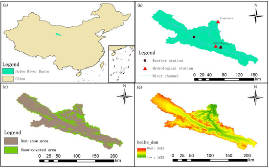
Figure 1.
Water system map of the upper reaches of the Heihe River Basin: (a) location in China, (b) river channel and stations, (c) land uses, and (d) DEM.
2.1.2. Data Collection
Basic data mainly include DEM data, meteorological data, hydrological data, and land use data. The resolution of DEM data is 90 m × 90 m, and the meteorological data mainly includes the rainfall data and daily average temperature data from meteorological stations in the watershed. The hydrological data mainly include the observed data of the hydrological stations, mainly including the daily flow series of the three hydrological stations: Zamashk, Qilian, and Yingluoxia. The length of both meteorological and hydrological data is from 2010 to 2019. The land use data comes from the new generation of EOS/MODIS satellite data. Considering the large amount of cloud cover, the eight-day synthetic snow cover product MOD10A1 of MODIS is used, and the spring snowmelt season (3–6 months) was chosen as remote sensing data period.
2.2. Model Description
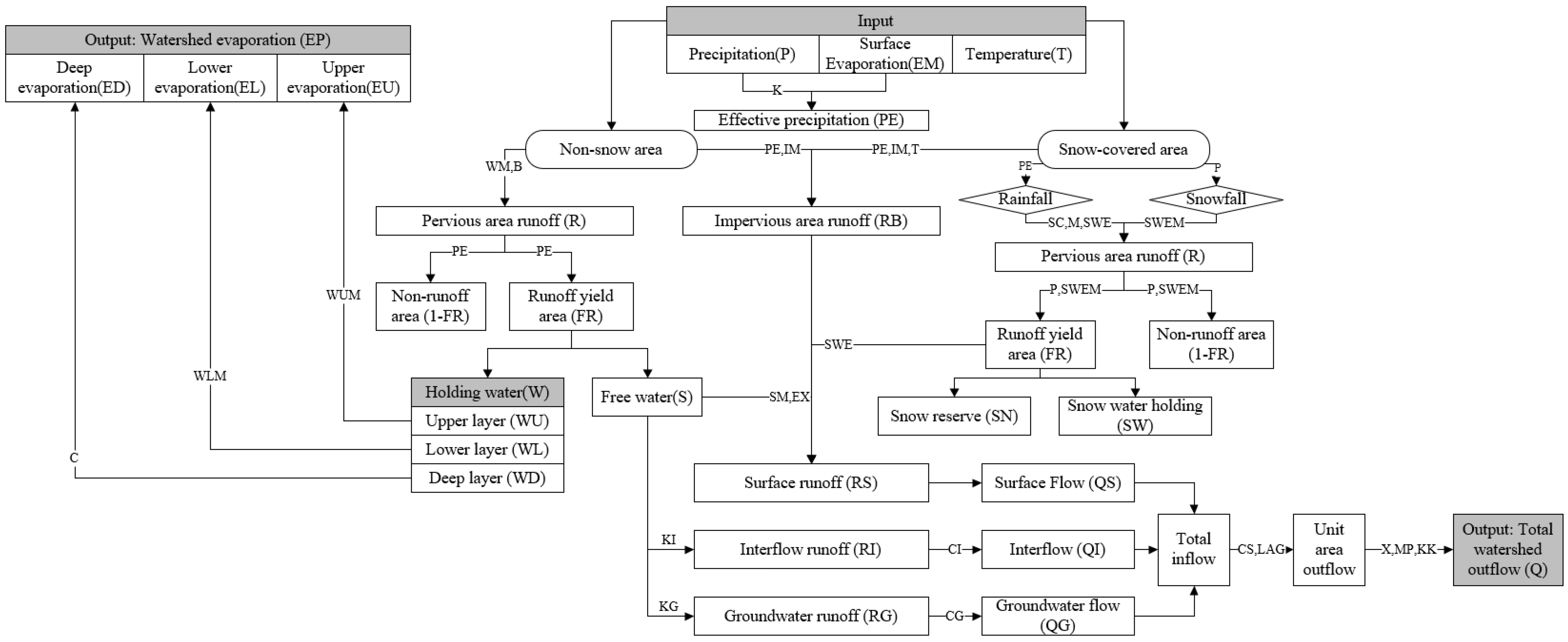
The traditional XHM includes four sub-models: evaporation, runoff yield, runoff separation, and runoff routing. In this study, the improved XHM is coupled with the snowmelt runoff module and some sub-models of the traditional XHM. Therefore, the watershed needs to be divided into two types, non-snow areas and snow-covered areas, because their runoff yield mechanisms are quite different, and need to be calculated separately. The non-snow areas are generally at lower elevations, while the snow-cover areas are generally at higher elevations. The snow-covered area also includes the glacier area, and its runoff yield mechanism is different from snow. The glacier area is considered as a higher average altitude than the snow area, and the precipitation is only in the form of snow. The general flowchart of the improved XHM model is shown in Figure 2.

Figure 2.
The flowchart of the improved XHM model.
2.2.1. Evaporation Sub-Model
The traditional three-level evaporation model is used in non-snow areas. The snow-covered areas are characterized by high altitudes and the average temperature is relatively low; thus, evaporation in these areas is not considered. Also, evaporation is not considered if the precipitation is in the form of snowfall because of the low temperature. If the precipitation is in the form of rainfall, evaporation needs to be considered. Generally, the relationship between watershed evaporation and water surface evaporation is linear, and water surface evaporation can be observed as follows:
where EP and EM are watershed evaporation and water surface evaporation, respectively. K is the evaporation conversion coefficient. The three-level evaporation is divided into the upper, lower, and deep layer, which is calculated as follows:
where EU, EL, and ED are the evaporation of the upper layer, lower layer, and deep layer. WL is the lower soil water content, WLM is the lower soil water-holding capacity, and C is the deep layer evaporation conversion coefficient.
2.2.2. Runoff Yield Sub-Model
- (1)
- Precipitation input processing
Precipitation usually includes rainfall and snowfall. The division of rainfall and snowfall is a crucial part of the improved XHM, mainly done by comparing the daily average temperature with the critical temperature of snowmelt. When the daily average temperature is greater than the critical temperature, all precipitation on that day is treated as rainfall. Otherwise, all precipitation on that day is treated as snowfall:
where Pt is the precipitation on the tth day; Prain,t is the precipitation in the form of rainfall on the tth day; Psnow,t is the precipitation in the form of snowfall on the tth day; Tt is the daily average temperature on the tth day; and Tc is the critical temperature for the division of rain and snow.
- (2)
- Snowmelt runoff module
The degree-day factor method is widely used when calculating snowmelt runoff. It is mainly based on the empirical relationship between glacier or snow melt and air temperature. Therefore, the degree-day model can be constructed and only the air-temperature value is needed:
where SWEM represents the maximum snow water equivalent; that is, the total amount of liquid water formed by the complete melting of snow. asnow represents the snowmelt degree-day factor (mm/(°C·d)), which represents the depth of snow melting when the temperature rises by 1 °C. Tmelt,snow is the threshold temperature for snow melting.
- (3)
- Runoff production calculation considering snow melting
The crucial point of runoff production is to judge whether the precipitation falls in the snow-covered areas or the non-snow areas, and their runoff yield mechanisms are quite different.
- Non-snow areas
According to the DEM and land use data of the study area (Figure 1), the non-snow areas are mainly distributed in the relatively lower altitude region with a relatively higher average temperature. According to the long-series meteorological data, the form of precipitation is mainly rainfall in non-snow areas and there are few snowfall events, and the snowfall amount of a single snowfall event is generally small and not enough to form long-term snow cover. Based on this, we assume that the runoff production of non-snow areas follows the principle of traditional runoff production under saturated conditions:
where PErain is the effective rainfall, W is the soil–water content of the watershed, WM is the average water-holding capacity of the watershed, and WMM is its maximum value. A is the ordinate value corresponding to the watershed water-holding-capacity curve. B is the uneven coefficient of the water-holding capacity of the watershed. All variables in the above formulas are in mm.
- b.
- Snow-covered areas (considering glaciers)
These areas are usually characterized as high altitude and the snow does not melt all year round. The runoff mechanism involves the maximum snowmelt water equivalent, actual snowmelt water equivalent, snow storage capacity, and snow water-holding capacity [39]. Moreover, the precipitation in the forms of either rainfall or snowfall in these areas is also different and needs further discussion.
- Case 1: the precipitation form is rainfall.
It should be stated that the glacier area has a lower average temperature, even lower than the snow area; therefore, precipitation in the glacier area is considered as snowfall (see Case 2). That is, we do not consider the rainfall on glaciers.
Here, the source of runoff not only comes from the remaining water after the rainfall fills the gaps of the snow but also comes from the melting of the snow itself. That is, the rainfall first fills the gaps of snow, and when the water storage capacity reaches the snow water-holding capacity, the remaining water will be discharged under gravity. Snow water-holding capacity is the same as soil water-holding capacity, and it also has uneven distribution. We use M to represent the uneven coefficient of snow water-holding capacity. The melting of the snow itself is the actual snowmelt water equivalent, obtained by comparing the actual snowmelt water equivalent with that of the previous day. The amount of runoff yield can be expressed by the following formula:
where Rsnow,t is the total runoff yield of the snow-covered areas; SWE is the actual snowmelt water equivalent; SN is the snow reserve; SW is the total amount of water held by the snow; SC is the average water-holding capacity of the snow and SCM is its maximum value; A0 is the ordinate value corresponding to the snow water-holding-capacity curve. All variables in the above formulas are in mm. The snowmelt yield here comes from the contributions of rainfall (PE) and snow melt (SWE), where SWE is a function of degree-day factor and temperature and has nothing to do with rainfall.
We assume that the change of SN is related to the change in temperature, and the specific calculation rules are as follows:
- If the threshold temperature for snow melting (Tmelt,snow) is between the temperature range of two adjacent days (hereby Tt and Tt−1), then
- If both Tt and Tt−1 are greater than Tmelt,snow then
- If both Tt and Tt−1 are less than Tmelt,snow then
- Case 2: the precipitation form is snowfall.
Here, snowfall is stored on the existing snow cover as part of total SN. The water yield from snow melting (Rsnow1,t) is calculated as follows:
The glacier runoff is divided into two types, debris-covered glaciers and debris-free glaciers, because they have different melting rates [40]. The glacier runoff is calculated as follows:
where
where GWEMt is the maximum glacier water equivalent, and Rdc,t and Rdf,t are the runoff from debris-covered and debris-free areas, respectively. GlacFrc is the proportion of glacier area to the whole watershed. Fdc and Fdf are the proportion of both debris-covered glaciers and debris-free glaciers, respectively. adc and adf are the degree-day factors of both debris-covered glaciers and debris-free glaciers, respectively. Tmelt,ice is the critical temperature of ice melting.
Similar to snow cover reserve (SN), the calculation of glacier cover reserve (GN) can refer to Equations (10)–(12). Similarly, the actual glacier water equivalent (GWE) is calculated as follows:
The total runoff considering both snow and glacier areas (Rsnow) is calculated as follows:
- Case 3: no precipitation.
At this time, the runoff is only derived from the snowmelt and glacier water equivalent, which is a function of both SN and GN, and the snowmelt and glacier water equivalent of the previous day, and the snowmelt runoff is calculated as follows.
2.2.3. Runoff Separation Sub-Model
This sub-model is still divided into surface runoff (RS), soil interflow runoff (RI), and groundwater runoff (RG), but they differ in non-snow areas and snow-covered areas. For runoff in non-snow areas, only rainfall runoff is considered, and the area ratio of runoff yield (FR) only considers the runoff generated by rainfall:
where Rrain is the total runoff yield in non-snow areas. For runoff in snow-covered areas, its main source mainly includes the surface snow melting and precipitation in the form of snowfall, and FR is calculated as follows:
where Psnow is precipitation in the form of snowfall; and Rsnow is the total runoff yield in snow-covered areas.
Correspondingly, RS in the non-snow areas (hereby RSrain) is calculated below:
RI and RG in non-snow areas (hereby RIrain and RGrain) are calculated as follows:
where KI and KG are the discharge coefficients of soil interflow runoff and groundwater runoff, respectively. The formula in the snow-covered areas (hereby RSsnow, RIsnow, and RGsnow) can refer to that in non-snow areas. However, the glacier runoff is considered as having no soil interflow runoff (RI) because the soil is frozen. Some of the glacier runoff is infiltrated into groundwater and the rest is the surface water; the coefficient of glacier melt runoff (θ) is used to define them. The total runoff in the snow area is as follows:
where S is the free water content of the soil, SM is the free water-holding capacity of the soil, and MS is its maximum value. AU is the ordinate value corresponding to the free water-holding-capacity curve. EX is the uneven coefficient of the free water-holding capacity of the soil.
2.2.4. Runoff Concentration Sub-Model
The principle of the runoff concentration sub-model is still divided into three stages: slope concentration, river network concentration, and river channel concentration. However, in the XHM considering snowmelt runoff, the calculation is performed after combining the RS, RI, and RG of both non-snow areas and snow-covered areas, namely:
The slope concentration stage is to convert runoff (R, mm) into flow (Q, m3/s). Correspondingly, RS, RI, and RQ should be converted into QS, QI, and QG:
where QS, QI, and QG are surface flow, soil interflow, and groundwater flow, respectively; U is the conversion factor from mm to m3/s, and ; F is the total area of the watershed (km2); and CI and CG are the extinction coefficient of interflow and groundwater flow, respectively.
In the river network concentration stage, the total flow is calculated as follows:
where
where Q is the total flow considering surface flow, soil interflow, and groundwater flow; CS is the extinction coefficient of surface flow; and L is the lag time.
The river channel concentration stage is calculated by the Muskingum method:
Where I and Q are the upstream flow and downstream flow, respectively; and C0, C1, and C2 are Muskingum calculation coefficients.
2.3. Model Calibration and Validation
2.3.1. Parameters Needing Calibration
In traditional XHM, 27 parameters need to be calibrated, covering four sub-models. If the snowmelt factor is considered, nine more parameters (SC, M, Tc, Tmelt,snow, Tmelt,ice, θ, asnow, adc, and adf) should be calibrated and only cover the runoff yield sub-model. The detailed parameter variables are listed in Table 1.

Table 1.
Parameter list of XHM.
2.3.2. Parameter Value Range Considering Snowmelt
- (1)
- Degree-day factor (a)
According to previous research and experience, there are two methods to calculate the degree-day factor: one is obtained through field observation, and the other is through empirical formula. The specific calculation method is as follows:
where ρs and ρw refer to the density of snow and water, respectively. According to Equation (34), as the density of water is fixed, the value of the degree-day factor directly only depends on the density of snow. Based on the observation data of relevant scholars from the east side of the Tianshan Mountains in Xinjiang and the Kunes River Valley, the snow density is stable between 0.06 and 0.24 g/cm3 [41]. If the altitude is higher, the snow will be more stable and the density will be higher correspondingly, about 0.3 to 0.35 g/cm3 [39,41]. In this paper, the value range of the degree-day factor of snow (asnow) is set between 0.6 and 3.5.
Considering the density of ice is larger than snow, the range of both adc and adf is set between 7.5 and 9.5.
- (2)
- Snow cover storage (SN)
SN is a state variable, and it changes with seasons. In general, the value of SN is higher and ranges from 30 to 50 mm in winter and spring because of the relatively lower temperature with the relatively thicker snow cover. Even in summer, the value of SN ranges from 10 to 20. That is because of the higher altitude with relatively lower temperatures in plain areas and the snow is not easy to completely melt. During simulation, the value of SN ranges from 10 to 50 depending on the simulation time.
2.3.3. Parameter Calibration and Model Assessment
The shuffled Complex Evolution Algorithm (SCE-UA) is used for parameter calibration, which can effectively solve the optimization problem with nonlinear constraints and obtain the global optimal solution of hydrological model parameters quickly and effectively, and has been widely used in the optimization of hydrological model parameters [42,43,44].
SCE-UA is a global optimization algorithm that combines the advantages of the simplex method and genetic algorithm, and it is designed to solve the problem that some local search algorithms often fall into the local extremum region and are difficult to converge to the global extremum region in the process of automatic parameter calibration of hydrological models [42]. In the SCE-UA algorithm, the initial solution is divided into several groups according to certain rules, and the points in each group are organized in a data structure called “complex”. The points in each complex are selected according to the competition mechanism to form a simplex, and then the downhill simplex algorithm is used to search and calculate.
After the search is completed, all the points are put back into a buffer. The shuffle algorithm is used to rearrange the position of points in the buffer to complete the generation evolution. After the completion of one generation of evolution, the SCE-UA algorithm shuffles the points in the buffer, disturbs the original order, and then redistributes the points in the buffer into several complexes according to the established rules, and then starts a new generation of evolution calculation. This process of assigning the points in the buffer to the complex, putting them back after evolution, and then shuffling is the mechanism of sharing information among the complex of the SCE-UA algorithm [45].
To assess the simulation efficiency of XHM, the determination coefficient (R2), mean square error (MSE), and Nash efficiency coefficient (NSE) were used.
where Qobs and Qsim represent the observed flow and simulated flow, respectively. Generally, if R2 is greater than 0.6 and NSE is greater than 0.5, the simulation effect can be considered satisfactory. If the NSE is above 0.75, the simulation effect is considered to be preferable [45]. For MSE, a value close to 0 means a better simulation result.
3. Results
3.1. Parameter Calibration Result
The daily hydrological data of the Zamashk and Yingluoxia stations from 2010 to 2016 were selected as the XHM’s calibration period, and from 2017 to 2019 was selected as its validation period. The parameters of the two stations were calibrated with the time step (Δt) of 6 h. The calibration results are shown in Table 2 and Table 3.

Table 2.
Calibration results of evapotranspiration, runoff yield and separation, and runoff concentration from slope and river network.

Table 3.
Calibration results of runoff concentration from river channel using Muskingum method of Yingluoxia station.
To illustrate, the total flow of both Yingluoxia and Zamashk is calculated as follows:
where QZ, QQL, QYLX are the simulated flow of the Zamashk, Qilian, and Yingluoxia stations. Qwtshd,Z and Qwtshd,QL are the upstream watershed input of the corresponding station. QQL,in and QZ,in are the flow inputs of the river channel from the Zamashk and Yingluoxia stations measured by the Muskingum method. Qwtshd,1 is the upstream watershed input bounded by the Zamashk, Qilian, and Yingluoxia stations. Therefore, Equations (22)–(24) indicate that the model output of Zamashk has only watershed input (Qwtshd,QL) that is related to evaporation, runoff yield and separation, and runoff concentration of the slope and river network, while the model output of Yingluoxia includes not only watershed input (Qwtshd,1) but also runoff concentration input of the river channel from the Zamashk (QZ,in) and Qilian (QQL,in) station. The topological graph of the hydrological stations is shown in Figure 3.
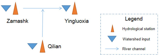
Figure 3.
The topological graph of the hydrological stations.
3.2. Model Simulation Result and Comparison
3.2.1. Model Efficiency Assessment
According to the calibrated parameter results, data from 2017 to 2019 were used for validation. In addition, to further illustrate the simulation effect of the XHM considering snowmelt, the traditional XHM was used for calibration and verification with the same dataset to further verify the simulation effectiveness. The results are shown in Table 4.

Table 4.
Calibration and inspection evaluation factor results of hydrological stations.
As can be seen in Table 4, in terms of the overall simulation results of two stations, XHM coupled with snowmelt has higher simulation accuracy than the traditional XHM, reflected by the higher values of R2 and NSE compared with traditional XHM under the same conditions, while the values of MSE are lower than the traditional XHM. Specifically, the values of R2 and NSE simulated by the traditional XHM in the Zamashk station are only about 0.4 and 0.2, respectively. Although the R2 of the Yingluoxia station reached about 0.7 under the traditional XHM, the NSE value did not exceed 0.6, and the simulation effect was satisfactory. When it comes to the XHM considering snowmelt, the R2 and NSE of Zamashk were close to 0.8 and 0.6, respectively, and that of the Yingluoxia station was about 0.8. In the case of MSE, the values of improvement are lower than the values of the traditional XHM. The MSE of the Yingluoxia station is also less than that of the Zamashk station because the downstream simulation effect is better than the upstream. Thus, the values of three indicators of different models in both calibration and validation processes suggest that the simulation results can restore the natural runoff process. The evaluation index of the XHM considering snowmelt is generally greater than that of the traditional XHM model in both calibration and validation periods. However, the simulation effect of Yingluoxia is better than that of Zamashk under both models, which may be because the simulation effect of the flow from watershed input (hereby Qwtshd,Z and Qwtshd,1) is poorer than that of the flow from river channel (hereby QZ,in and QQL,in), because there are more parameters related to the flow from Qwtshd,Z and Qwtshd,1 compared with that from QZ,in and QQL,in, and the snowmelt runoff also comes from the Qwtshd,Z and Qwtshd,1. Besides the watershed input Qwtshd,1, the flow of Yingluoxia also includes the inflow input of QZ,in and QQL,in, while the flow of Zamashk itself only from Qwtshd,Z, resulting in its relatively poor simulation effect.
3.2.2. Comparison of Simulation Result with the Traditional Model
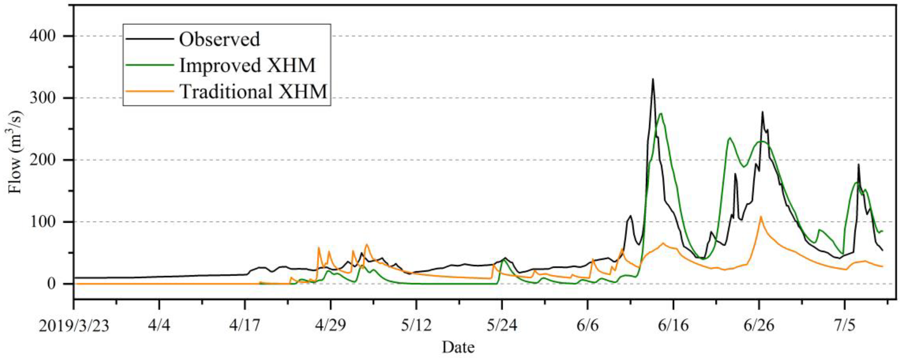
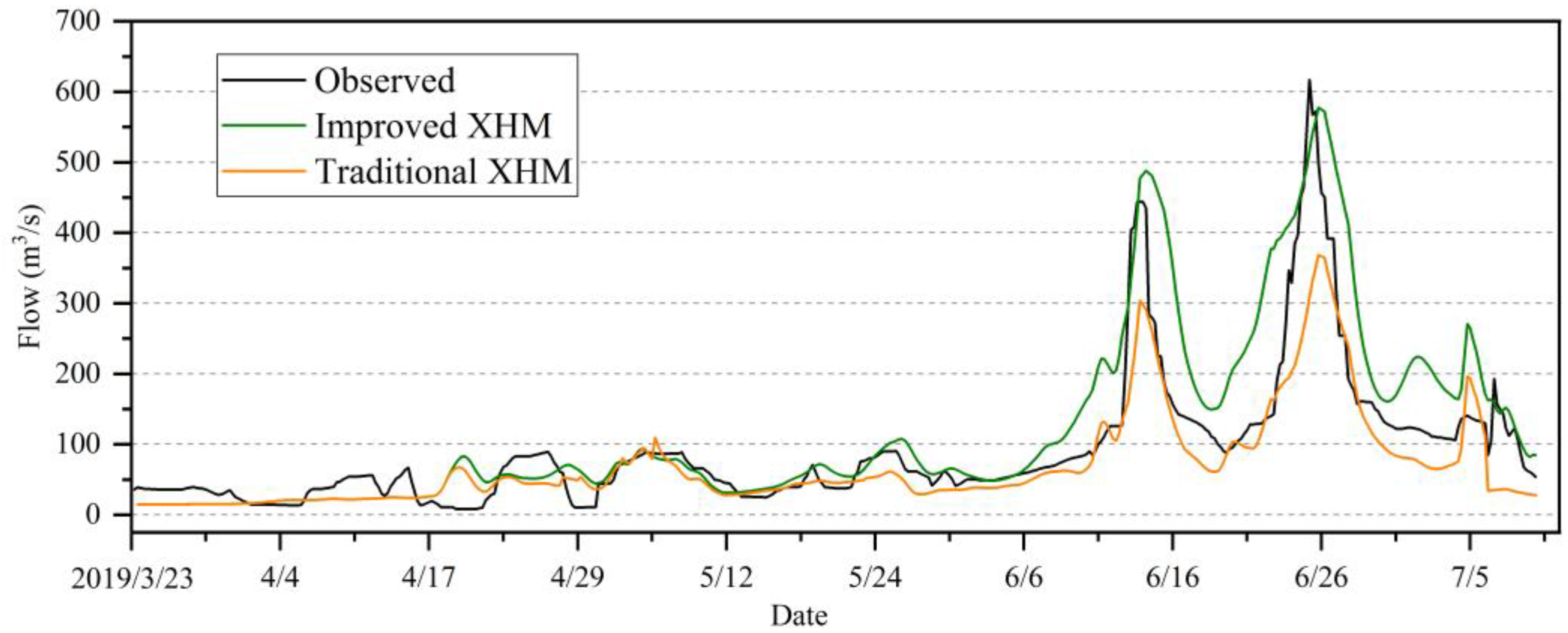
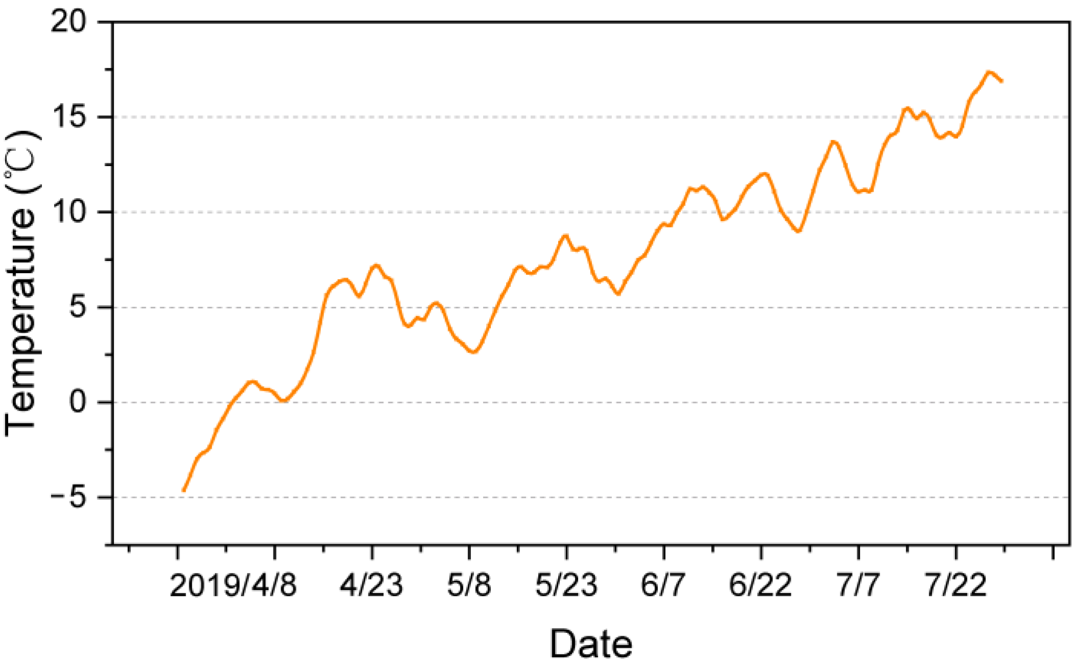
To illustrate the simulation effect of the flooding process, the flood process simulation results of the traditional XHM of 2019 were compared with the simulation results using the XHM coupled with snowmelt runoff presented in this paper, and the simulation results of Zamashk and Yingluoxia stations were shown in Table 5, Figure 4 and Figure 5, respectively. The flooding process of 14~17 June, 24~27 June, and 5~8 July can be well simulated by the XHM with coupled snowmelt runoff. It can also be seen that the observed flood peak of the Yingluoxia station on 14~17 June was about 444 m3/s, and the flood peak simulated by the traditional XHM was only about 303 m3/s, indicating that the difference between the flood peak of both observed and simulated values with the traditional model is basically from snowmelt runoff. We can see from Table 5 that the error of the flood peak value of 14~17 June simulated by the improved XHM is only 10% compared with the traditional XHM of 32%, while the error of the flood peak value of 24~27 June simulated by improved XHM is only 6% compared with the traditional XHM of 40%, indicating that both flood process and flood peak could be well simulated using the improved XHM in this paper. However, the peak flow simulation of the Zamashk station is poorer than that of the Yingluoxia station. For example, the error of the peak flood of 24~27 June of the Zamashk station is 18%, which is larger than that of the Yingluoxia station at 6%, and the evaluation factors of the Zamashk station are also poorer than Yingluoxia (Table 4). This is because there is only watershed input (Qwtshd,Z) for Zamashk with more parameters and limited accuracy. From the analysis of air temperature data, there was a period of temperature rise of about 5 °C from 9 June to 14 June (see Table 6), and the watershed is almost covered by snow, which further determined that the difference in flow was due to the snowmelt runoff.

Table 5.
The peak flow simulation and occurring time of both flood processes using different models.
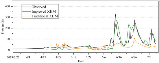
Figure 4.
Comparison of flood simulation results using different methods at Zamashk Station in 2019.
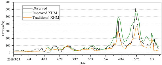
Figure 5.
Comparison of flood simulation results using different methods at Yingluoxia Station in 2019.

Table 6.
Daily temperature in June.
It should be noted, however, that the setting of the model state variable SN is very crucial because the source of snowmelt runoff in the northwest is mostly SN. We can see that the flood on 5 July was not as large as the previous two floods. This is because the corresponding rainfall is relatively low, but the temperature is relatively higher in July. If the SN was too large, the simulated runoff on 5 July would also be large as there was a large snow reserve at the model’s initial state, and there might be a certain snow reserve on 5 July. As temperatures rise, snow melts, creating more snowmelt runoff. However, according to the analysis of observed rainfall and hydrological data, the flood contribution on 5 July is mainly the rainfall from the watershed (Qwtshd,1) and the upstream flow (QZ,in and QQL,in). In addition, the temperature will rise in July, and there will be fewer snow reserves in the watershed in June or July compared with the beginning of the year. However, when SN is too small, the snowmelt flood process cannot be simulated because there is no snow cover on the soil at this time, and the runoff is still dominated by rainfall from the watershed.
3.3. Flood Composition Analysis
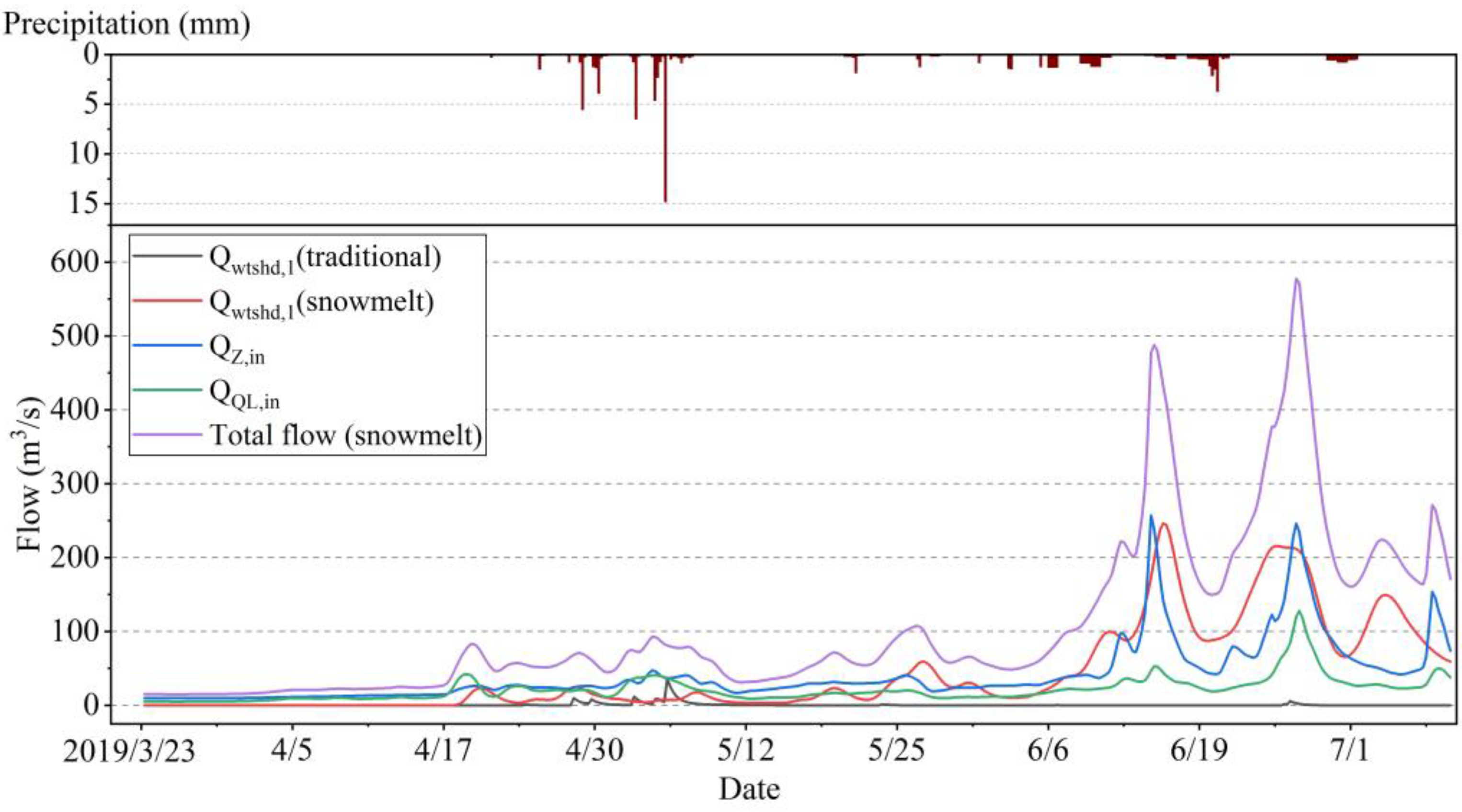
The flood composition analysis of the Yingluoxia station in 2019 is shown in Figure 6. As can be seen in Figure 6, the flow from the upstream watershed input (Qwtshd,1) simulated using the traditional XHM is basically zero, because there are few rainfalls from the upstream watershed. We can also see from Figure 6 that the precipitation in early May is larger than that of June, but the total flow is only about 100 m3/s, compared with the flood process in June with a flow peak of 488 m3/s and 577 m3/s, respectively. This is because the watershed is located in an arid area where annual evaporation is much greater than annual precipitation, resulting in a soil water shortage compared with humid areas. The precipitation will first replenish the soil water storage before the runoff is yielded in early May, and the snow cover of late spring initially reserved in the soil will transfer to runoff as the temperature rises and exceeds Tmelt in June (see Figure 7).

Figure 6.
Analysis of flood composition in 2019 at Yingluoxia Hydrological Station.

Figure 7.
The 5 day sliding average temperature process.
However, from the measured temperature analysis, the temperature increase of the second flood process was only 3 °C (from about 19 to 24 June), which is less than the temperature increase of 5 °C of the first flood process (see Table 6 and Figure 7), but the second peak flow was higher than the first peak flow. This is because the contribution of the second flood is from not only Qwtshd,1 but also QZ,in and QQL,in. The contribution of QQL,in in the second flood is larger than that of the first flood, while the contribution of QZ,in is almost the same. But in terms of Qwtshd,1, the peak flow of the second flood process is still lower than the peak flow of the first flood, probably as the temperature-increasing rate of the second flood process is less than that of the first flood process.
4. Discussion
4.1. Sensitivity Analysis of Parameters
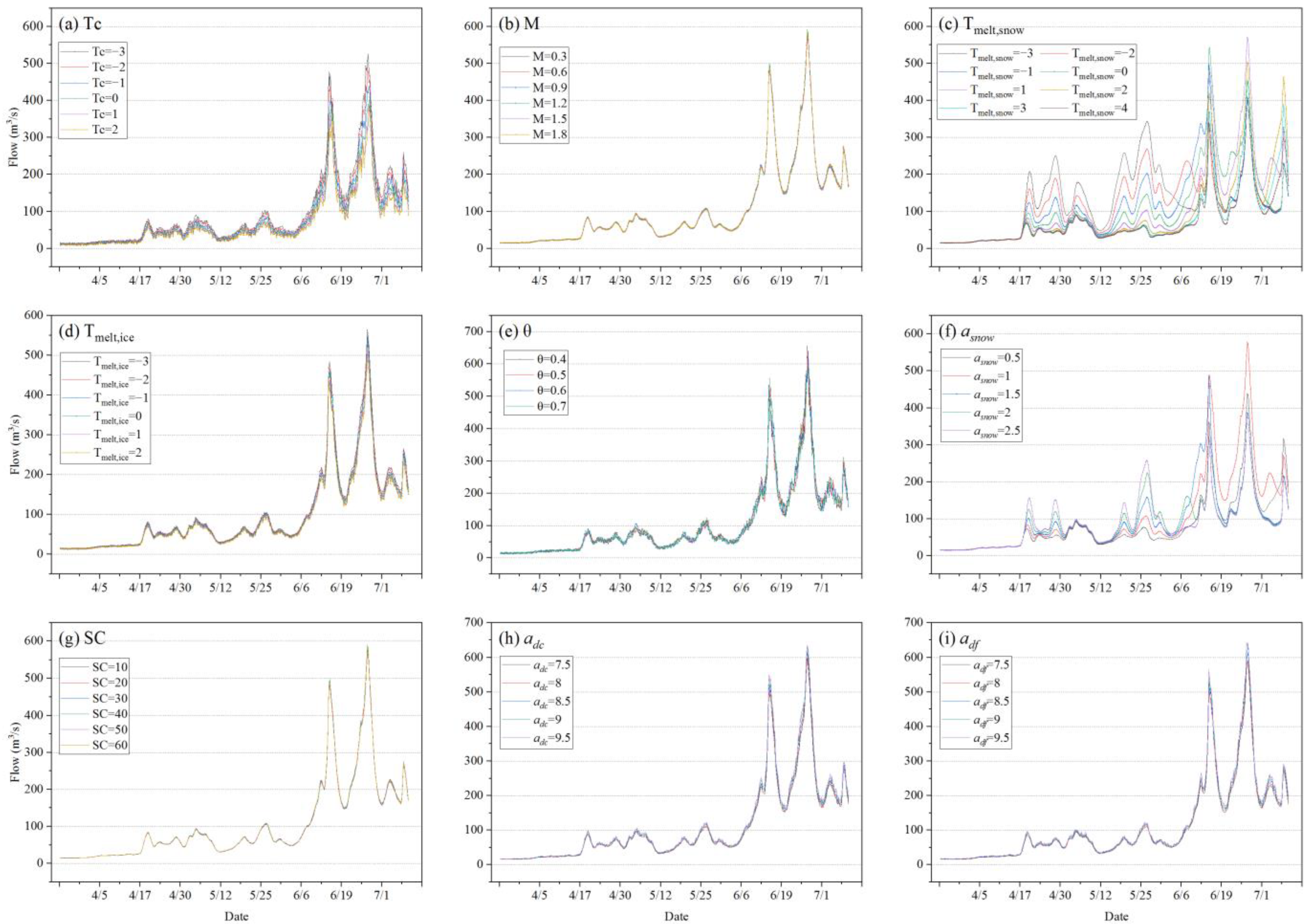
In this paper, the sensitivity analysis of nine parameters referring to the snowmelt module is shown in Figure 8. Figure 8a–i demonstrates the effects of the flow process of the Yingluoxia station on changing ranges of Tc, M, Tmelt,ice, Tmelt,snow, θ, asnow, SC, adc, and adf, respectively. It should be pointed out that we keep the other parameters unchanged (See Table 2) when we analyze one parameter. We can see that SC and M are not sensitive to the flood simulation results, while Tmelt,ice adc, adf, and θ are less sensitive to flood simulation results. This is because the snow density and snow water-holding capacity are relatively even, and the proportion of glaciers in the snow-covered area is small. In other words, Tmelt,ice and θ are related to glacier runoff, but there is little contribution of glacier runoff to total runoff because of the poor proportion of the glacier area. However, Tc, Tmelt,snow, and a are relatively sensitive to the flood simulation results, and the latter two are more sensitive. This is because the snow cover accounts for a large proportion, and the average temperature of the study area is hovering around the threshold temperature of snow melting.
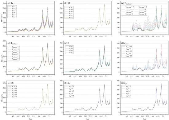
Figure 8.
Sensitive analysis: the effect of the flooding process of Yingluoxia station on changing parameters referring to snowmelt module: Tc, M, Tmelt,ice, Tmelt,snow, θ, asnow, adc, adf, and SC.
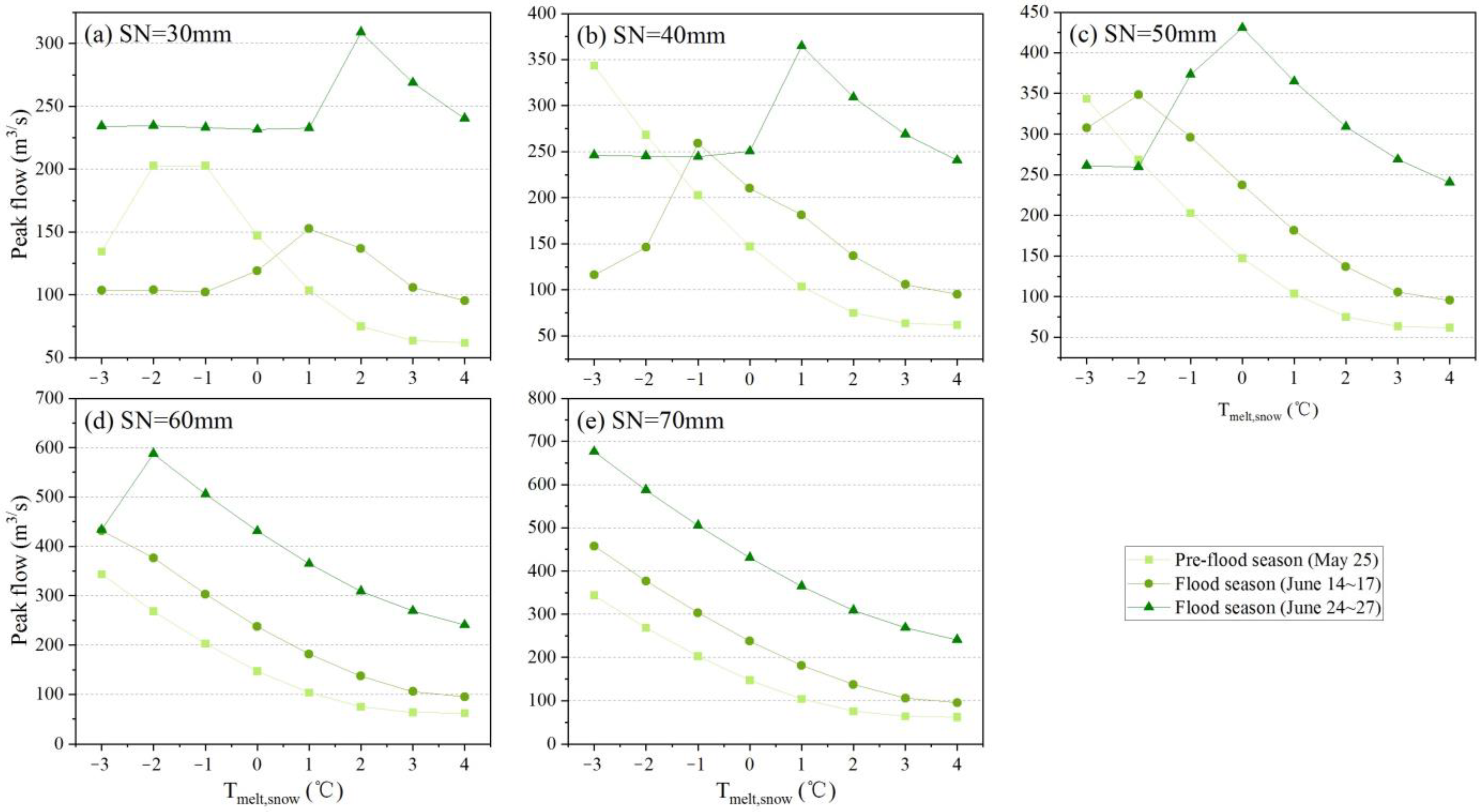
In addition, the amount of runoff and Tmelt,snow also have some regularity (Figure 8d). Concretely, there is relatively more snow reserve (SN) before flood season (about 1 June) and enough snow reserve for melting to runoff; thus, at the same moment, the lower the critical temperature of snow melt, the more snow is melting to river runoff. However, in flood season, such a relationship is no longer valid. For example, in the flooding process on 14~17 June, when the critical temperature of snowmelt is below 0 °C, the lower critical temperature of snowmelt results in less river runoff. This is because of the initial state and the initial snow reserve (SN) of the model (See Figure 9). If the initial SN is small, there is seldom snow cover in flood season, and runoff is only related to precipitation at this time and has nothing to do with temperature.

Figure 9.
The effect of the peak flows of three different flood processes of Yingluoxia station under varying critical temperatures of snow melting (Tmelt,snow) on different model’s initial states (SN).
Moreover, the same story occurs in the analysis of the degree-day factor. The higher value of the degree-day factor represents more snow melting to river runoff (Figure 6). This occurs in the pre-flood season where there is more snow reserve. When it comes to the flood season, the total runoff only refers to precipitation and has nothing to do with degree-day factor and Tmelt, snow, unless there is more snow reserve at the beginning. That is, if there’s more snow reserve, total runoff relates to precipitation, Tmelt, snow, and degree-day factor, otherwise, it is only related to precipitation and other non-snow parameters.
4.2. Effects of Model’s State
We stated in the previous section that the lower critical temperature of snow melting (Tmelt,snow) will result in higher snowmelt runoff, but this is valid only in a certain model state. Here, we selected three flood processes (one for the pre-flood season on 25 May, the other two for the flood seasons on 14~17 and 24~27 June, respectively) to analyze the peak flow trend in the Yingluoxia station by varying Tmelt,snow under different model states, that is, a different value of initial snow reserve (SN) ranging from 30 mm to 70 mm with the step of 5 mm. The analyzing results are shown in Figure 9. We can see from Figure 9 that the peak flows of the three flood processes show a decreasing trend as Tmelt,snow increases only when SN equals 70 mm or more. When SN decreases, only some of the flood processes conform to this law. For example, when SN equals 60 mm, only the first two floods meet this principle. But when SN equals 50 mm or 40 mm, only the first flood meets this principle. To illustrate, more SN means more snow reserves, and such a relationship between Tmelt,snow and peak flow stands only when there are enough snow reserves. As SN decreases, the flood process of pre-flood season is more likely to make such a relationship work compared with that in flood season, because there is more snow reserve than in the flood season with a higher average temperature.
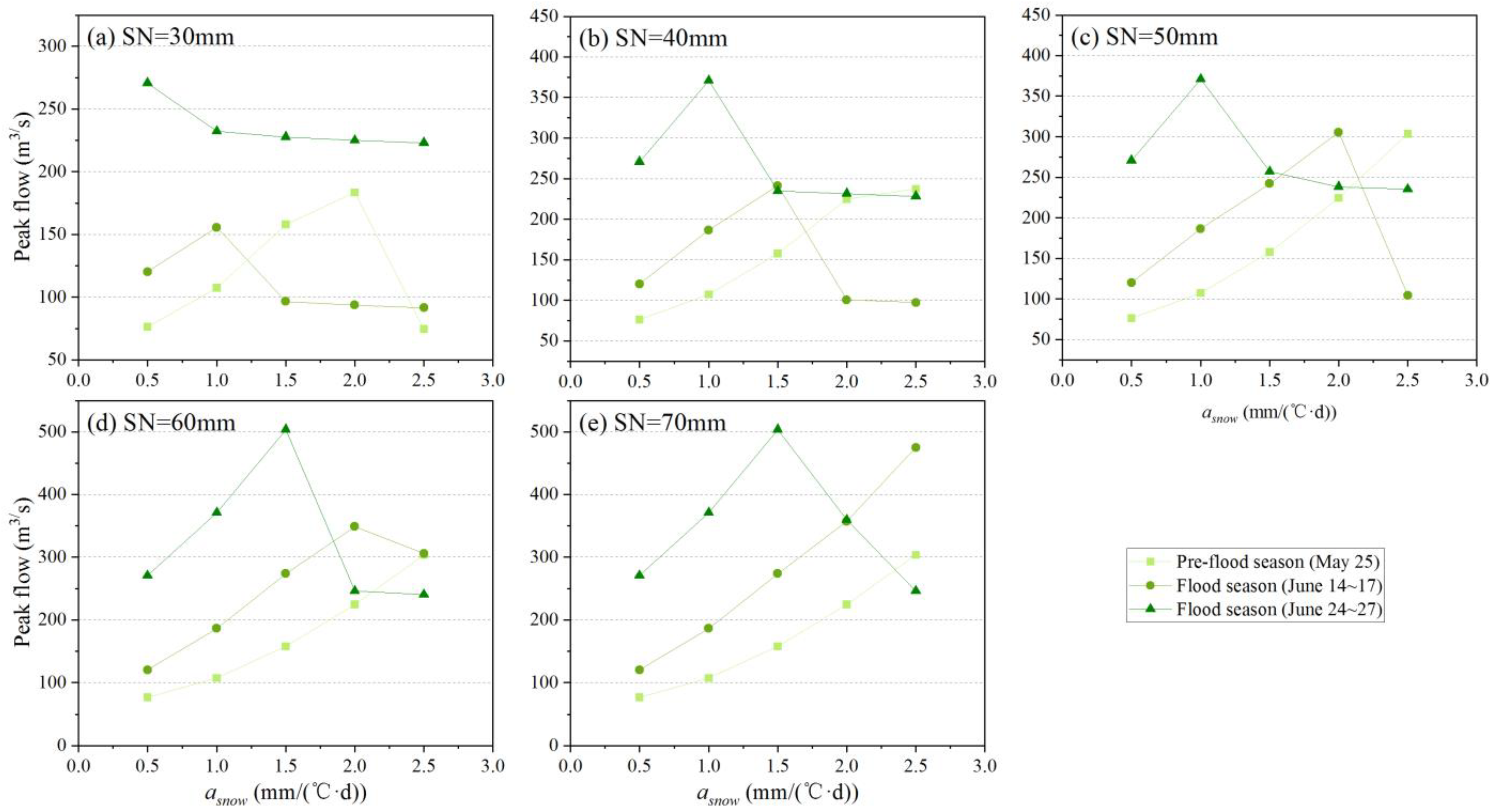
Besides Tmelt, snow, the impact of different flow processes of varying degree-day factors of snow (asnow) are also analyzed and shown in Figure 10. Generally, a greater degree-day factor will generate more snowmelt runoff. However, this only occurs when there is enough snow reserve, which is similar to the analysis of Tmelt,flow. The third flood process accords with this relationship only when the degree-day factor is less than 1.5 under an initial SN equal to 70 mm, while the first two flood processes accord with this relationship (Figure 10e). As the SN decreases, the earlier floods (25 May and 14~17 June) are more likely to conform to this rule compared with the flood process on 24~27 June. This is also due to more snow reserve in the earlier floods with lower temperatures under the same initial SN.

Figure 10.
The effect of the peak flows of three different flood processes of Yingluoxia station under varying critical degree-day factors of snow (asnow) on different model’s initial states (SN).
4.3. Model Comparisons and Limitations
Currently, the main method of simulating the snow melt runoff is the SRM model [6], SPHY model [33], and frozen soil hydrological model, which separates the total flow calculation from both rainfall and snowfall (including snow reserve in the basin). That is, the whole process of both runoff yield and concentration is calculated in the precipitation and snowmelt areas respectively; thus, both the area of the total watershed and the snow-covered part are needed in the model. However, in this research, the non-snow area and snow-covered areas are separated only in the runoff yield calculation process. The input of the runoff separation module involves the summary of both rainfall and snow-melt runoff; thus, only the total area of the watershed is needed. Therefore, this study seems to improve the model where there is no snowmelt module, but it still follows the advantages of the traditional model [28,29].
Although this research presented the improved Xin’anjiang model considering the snowmelt module and further expanded the application scope in areas with different traditions, there are still some limitations of this study. For example, the division of precipitation forms of either rainfall or snowfall is defined only by the critical temperature. However, as the precipitation falls from the sky to the ground, the temperature will rise. If the precipitation in the sky is in the form of snow, it may convert to rain when it falls to the ground. In addition, the traditional XHM is presented based on the water balance of the river basin, but the water balance equation may still be valid in snow-covered areas. These points will be considered in future research on the development of hydrological modeling considering snow and glacier runoff.
5. Conclusions
Based on the traditional XHM, the snowmelt runoff module is considered to study the mechanism of runoff yield and concentration of snow-dominated areas by dividing the watershed into non-snow areas and snow-covered areas. The flood process was simulated in the upper reaches of the Heihe River basin in northwest China, and the following conclusions were obtained:
First, the index of the model’s performance in the improved model is superior to that of the traditional model. The flood processes can be better simulated and the peak flow in two flood processes in June is almost near the observed value. This shows that the model can be applied in the Heihe River Basin and provides important technical support for flood forecasting in Northwest China and other regions dominated by snowmelt runoff, which expands the model’s application scope, provides a strong tool for flood forecasting in snow-dominated areas, and provides certain technical references for flood forecasting and early warning.
Second, flood composition analysis indicates that the watershed input simulation is not as good as the river channel’s simulation result because of the numerous parameters of watershed input which limited the model’s prediction accuracy when there is only upstream watershed input, reflected by the relatively poor simulated effect of the Zamashk station compared with the Yingluoxia Station. Further research should emphasize the water balance of snow cover, the deeper characteristics of the runoff yield of snowmelt, and the mechanism of runoff yield when snowfall transfers to rainfall as the temperature near the ground is higher than that in the upper air to further improve the accuracy of flood forecasting.
Finally, sensitivity analysis indicates that of the nine parameters related to snow melting, only the critical temperature of snowmelt and the degree-day factor of snow are sensitive to the simulated runoff process, and its changing trend is related to the model’s initial state, i.e., the initial snow reserve. Both the decrease in the critical temperature of the snowmelt and the increase in the degree-day factor will lead to the increased trend of the peak flood, but such a relationship stays true only when there is enough snow reserve caused by either the higher value of initial SN or a flood that occurs in the pre-flood season, providing strong references for researchers for setting model’s parameters and initial states.
Author Contributions
Conceptualization: Y.T. and A.H.; Dataset: W.Y.; Methodology: A.H. and Y.T.; Calibration and Validation: N.D.; Writing: Y.T.; Supervision: A.H. and N.D. All authors have read and agreed to the published version of the manuscript.
Funding
This research was funded by National Key Research Plan (2021YFB3900601) and the Natural Science Foundation of Henan (232300421250).
Data Availability Statement
Not applicable.
Acknowledgments
We would like to express our sincere thanks to the anonymous reviewers.
Conflicts of Interest
The authors declare no conflict of interest.
References
- Mook, W.G. Environmental Isotopes in the Hydrological Cycle: Principles and Applications; UNESCO: Paris, France, 2000. [Google Scholar]
- Paz-Ríos, C.E.; Sosa-López, A.; Torres-Rojas, Y.E. Spatiotemporal Configuration of Hydrographic Variability in Terminos Lagoon: Implications for Fish Distribution. Estuaries Coasts 2023. [Google Scholar] [CrossRef]
- Shi, W.; Qiu, J.; Zhang, C.; Wang, Q.; Lai, J.; Li, B.; Mao, Z. Immersion mode and spatiotemporal distribution characteristic of water migration in loess tunnel. Arab. J. Geosci. 2022, 15, 654. [Google Scholar] [CrossRef]
- Bisht, N.; Chauhan, P.S. Excessive and disproportionate use of chemicals cause soil contamination and nutritional stress. In Soil Contamination-Threats and Sustainable Solutions; IntechOpen: London, UK, 2020; pp. 1–10. [Google Scholar]
- Zhu, G.; Wang, L.; Liu, Y.; Bhat, M.A.; Qiu, D.; Zhao, K.; Sang, L.; Lin, X.; Ye, L. Snow-melt water: An important water source for Picea crassifolia in Qilian Mountains. J. Hydrol. 2022, 613, 128441. [Google Scholar] [CrossRef]
- Meng, X.; Liu, Y.; Qin, Y.; Wang, W.; Zhang, M.; Zhang, K. Adaptability of MODIS Daily Cloud-Free Snow Cover 500 m Dataset over China in Hutubi River Basin Based on Snowmelt Runoff Model. Sustainability 2022, 14, 4067. [Google Scholar] [CrossRef]
- Marks, D.; Kimball, J.; Tingey, D.; Link, T. The sensitivity of snowmelt processes to climate conditions and forest cover during rain-on-snow: A case study of the 1996 Pacific Northwest flood. Hydrol. Process. 1998, 12, 1569–1587. [Google Scholar] [CrossRef]
- Li, M.; Weng, B.; Yan, D.; Bi, W.; Yang, Y.; Gong, X.; Wang, H. Spatiotemporal characteristics of surface water resources in the Tibetan plateau: Based on the produce water coefficient method considering snowmelt. Sci. Total Environ. 2022, 851, 158048. [Google Scholar] [CrossRef]
- Yang, W.; Chen, L.; Deng, F.; Lv, S. Application of an improved distributed Xin’anjiang hydrological model for flood prediction in a karst catchment in South-Western China. J. Flood Risk Manag. 2020, 13, e12649. [Google Scholar] [CrossRef]
- Hartmann, A.; Goldscheider, N.; Wagener, T.; Lange, J.; Weiler, M. Karst water resources in a changing world: Review of hydrological modeling approaches. Rev. Geophys. 2014, 52, 218–242. [Google Scholar] [CrossRef]
- Fleury, P.; Plagnes, V.; Bakalowicz, M. Modelling of the functioning of karst aquifers with a reservoir model: Application to Fontaine de Vaucluse (south of France). J. Hydrol. 2007, 345, 38–49. [Google Scholar] [CrossRef]
- Jukić, D.; Denić-Jukić, V. Nonlinear kernel functions for karst aquifers. J. Hydrol. 2006, 328, 360–374. [Google Scholar] [CrossRef]
- Hartmann, A.; Barberá, J.A.; Lange, J.; Andreo, B.; Weiler, M. Progress in the hydrologic simulation of time variant recharge areas of karst systems—Exemplified at a karst spring in Southern Spain. Adv. Water Resour. 2013, 54, 149–160. [Google Scholar] [CrossRef]
- Ronayne, M.J. Influence of conduit network geometry on solute transport in karst aquifers with a permeable matrix. Adv. Water Resour. 2013, 56, 27–34. [Google Scholar] [CrossRef]
- Usman, M.; Ndehedehe, C.E.; Farah, H.; Ahmad, B.; Wong, Y.; Adeyeri, O.E. Application of a Conceptual Hydrological Model for Streamflow Prediction Using Multi-Source Precipitation Products in a Semi-Arid River Basin. Water 2022, 14, 1260. [Google Scholar] [CrossRef]
- Beven, K.J.; Kirkby, M.J.; Freer, J.E.; Lamb, R. A history of TOPMODEL. Hydrol. Earth Syst. Sci. 2021, 25, 527–549. [Google Scholar] [CrossRef]
- Ambroise, B.; Beven, K.; Freer, J. Toward a generalization of the TOPMODEL concepts: Topographic indices of hydrological similarity. Water Resour. Res. 1996, 32, 2135–2145. [Google Scholar] [CrossRef]
- McMichael, C.E.; Hope, A.S.; Loaiciga, H.A. Distributed hydrological modelling in California semi-arid shrublands: MIKE SHE model calibration and uncertainty estimation. J. Hydrol. 2006, 317, 307–324. [Google Scholar] [CrossRef]
- Wang, S.; Zhang, Z.; Sun, G.; Strauss, P.; Guo, J.; Tang, Y.; Yao, A. Multi-site calibration, validation, and sensitivity analysis of the MIKE SHE Model for a large watershed in northern China. Hydrol. Earth Syst. Sci. 2012, 16, 4621–4632. [Google Scholar] [CrossRef]
- Arnold, J.G.; Moriasi, D.N.; Gassman, P.W.; Abbaspour, K.C.; White, M.J.; Srinivasan, R.; Santhi, C.; Harmel, R.D.; van Griensven, A.; Van Liew, M.W. SWAT: Model use, calibration, and validation. Trans. ASABE 2012, 55, 1491–1508. [Google Scholar] [CrossRef]
- Douglas-Mankin, K.R.; Srinivasan, R.; Arnold, J.G. Soil and Water Assessment Tool (SWAT) model: Current developments and applications. Trans. ASABE 2010, 53, 1423–1431. [Google Scholar] [CrossRef]
- Wang, Y.; Jiang, R.; Xie, J.; Zhao, Y.; Yan, D.; Yang, S. Soil and water assessment tool (SWAT) model: A systemic review. J. Coast. Res. 2019, 93, 22–30. [Google Scholar] [CrossRef]
- Gao, H.; Tang, Q.; Shi, X.; Zhu, C.; Bohn, T.; Su, F.; Sheffield, J.; Pan, M.; Lettenmaier, D.; Wood, E. Water budget record from Variable Infiltration Capacity (VIC) model. In Algorithm Theoretical Basis Document for Terrestrial Water Cycle Data Records; 2010; Available online: https://eprints.lancs.ac.uk/id/eprint/89407/1/Gao_et_al_VIC_2014.pdf (accessed on 8 August 2023).
- Zhang, Y.; You, Q.; Chen, C.; Ge, J.; Adnan, M. Evaluation of downscaled CMIP5 coupled with VIC model for flash drought simulation in a humid subtropical basin, China. J. Clim. 2018, 31, 1075–1090. [Google Scholar] [CrossRef]
- Kordilla, J.; Sauter, M.; Reimann, T.; Geyer, T. Simulation of saturated and unsaturated flow in karst systems at catchment scale using a double continuum approach. Hydrol. Earth Syst. Sci. 2012, 16, 3909–3923. [Google Scholar] [CrossRef]
- Reimann, T.; Rehrl, C.; Shoemaker, W.B.; Geyer, T.; Birk, S. The significance of turbulent flow representation in single-continuum models. Water Resour. Res. 2011, 47, W09503. [Google Scholar] [CrossRef]
- Okkan, U.; Ersoy, Z.B.; Kumanlioglu, A.A.; Fistikoglu, O. Embedding machine learning techniques into a conceptual model to improve monthly runoff simulation: A nested hybrid rainfall-runoff modeling. J. Hydrol. 2021, 598, 126433. [Google Scholar] [CrossRef]
- Hu, J.; Chen, S.; Behrangi, A.; Yuan, H. Parametric uncertainty assessment in hydrological modeling using the generalized polynomial chaos expansion. J. Hydrol. 2019, 579, 124158. [Google Scholar] [CrossRef]
- Zhang, D.; Quan, J.; Wang, F.; He, X. Flash flood simulation using geomorphic unit hydrograph method: Case study of headwater catchment of Xiapu River Basin, China. In Proceedings of the International Conference on Hydroinformatics, New York, NY, USA, 17–21 August 2014. [Google Scholar]
- Yao, C.; Ye, J.; He, Z.; Bastola, S.; Zhang, K.; Li, Z. Evaluation of flood prediction capability of the distributed Grid-Xin’anjiang model driven by weather research and forecasting precipitation. J. Flood Risk Manag. 2019, 12, e12544. [Google Scholar] [CrossRef]
- Zhao, Q.; Ye, B.; Ding, Y.; Zhang, S.; Yi, S.; Wang, J.; Shangguan, D.; Zhao, C.; Han, H. Coupling a glacier melt model to the Variable Infiltration Capacity (VIC) model for hydrological modeling in north-western China. Environ. Earth Sci. 2013, 68, 87–101. [Google Scholar] [CrossRef]
- Finsterwalder, S.; Schunk, H. Der suldenferner. Z. Des Dtsch. Und Oesterreichischen Alpenver. 1887, 18, 72–89. [Google Scholar]
- Singh, V.; Jain, S.K.; Shukla, S. Glacier change and glacier runoff variation in the Himalayan Baspa river basin. J. Hydrol. 2021, 593, 125918. [Google Scholar] [CrossRef]
- Matinec, J.; Rango, A. Parameter values for snowmelt runoff modeling. J. Hydrol. 1986, 84, 197–219. [Google Scholar] [CrossRef]
- Fathi, M.M.; Awadallah, A.G.; Aldahshoory, W. An Improved Monthly Water Balance GR2M Model with a Seasonally Variable Parameter. J. Hydrol. 2023, 617, 129127. [Google Scholar] [CrossRef]
- Maneechot, L.; Wong, Y.J.; Try, S.; Shimizu, Y.; Bharambe, K.P.; Hanittinan, P.; Ram-Indra, T.; Usman, M. Evaluating the necessity of post-processing techniques on d4PDF data for extreme climate assessment. Environ. Sci. Pollut. Res. 2023. [Google Scholar] [CrossRef] [PubMed]
- Gómez-Landesa, E.; Rango, A. Operational snowmelt runoff forecasting in the Spanish Pyrenees using the snowmelt runoff model. Hydrol. Process. 2002, 16, 1583–1591. [Google Scholar] [CrossRef]
- Li, X.; Cheng, G.; Ge, Y.; Li, H.; Han, F.; Hu, X.; Tian, W.; Tian, Y.; Pan, X.; Nian, Y.; et al. Hydrological cycle in the Heihe River Basin and its implication for water resource management in endorheic basins. J. Geophys. Res. Atmos. 2018, 123, 890–914. [Google Scholar] [CrossRef]
- Yin, Z.; Feng, Q.; Liu, S.; Zou, S.; Li, J.; Yang, L.; Deo, R.C. The spatial and temporal contribution of glacier runoff to watershed discharge in the Yarkant River Basin, Northwest China. Water 2017, 9, 159. [Google Scholar] [CrossRef]
- Yan, W. Study on Variations of Runoff and Its Components in Three Sources Streams of Tarim River. Master’s Thesis, Xi’an University of Technology, Xi’an, China, 2021. [Google Scholar]
- Zhang, Y.; Liu, S.; Ding, Y. Observed degree-day factors and their spatial variation on glaciers in western China. Ann. Glaciol. 2006, 43, 301–306. [Google Scholar] [CrossRef]
- Xu, Y.; Liu, C.; Yu, Q.; Zhao, C.; Quan, L.; Hu, C. Study on a Hybrid Hydrological Forecasting Model SCE-GUH by Coupling SCE-UA Optimization Algorithm and General Unit Hydrograph. Water 2023, 15, 2783. [Google Scholar] [CrossRef]
- Arsenault, R.; Poulin, A.; Côté, P.; Brissette, F. Comparison of stochastic optimization algorithms in hydrological model calibration. J. Hydrol. Eng. 2014, 19, 1374–1384. [Google Scholar] [CrossRef]
- Kan, G.; He, X.; Li, J.; Ding, L.; Hong, Y.; Zhang, H.; Liang, K.; Zhang, M. Computer aided numerical methods for hydrological model calibration: An overview and recent development. Arch. Comput. Methods Eng. 2019, 26, 35–59. [Google Scholar] [CrossRef]
- Duan, Q.; Sorooshian, S.; Gupta, V. Effective and efficient global optimization for conceptual rainfall-runoff models. Water Resour. Res. 1992, 28, 1015–1031. [Google Scholar] [CrossRef]
Disclaimer/Publisher’s Note: The statements, opinions and data contained in all publications are solely those of the individual author(s) and contributor(s) and not of MDPI and/or the editor(s). MDPI and/or the editor(s) disclaim responsibility for any injury to people or property resulting from any ideas, methods, instructions or products referred to in the content. |
© 2023 by the authors. Licensee MDPI, Basel, Switzerland. This article is an open access article distributed under the terms and conditions of the Creative Commons Attribution (CC BY) license (https://creativecommons.org/licenses/by/4.0/).


