Effects of Urbanization on Changes in Precipitation Extremes in Guangdong-Hong Kong-Macao Greater Bay Area, China

Abstract

Complex interaction between urbanization and climate change has been showing significant impacts on natural and human ecosystems. Increasing urban flooding and waterlogging are associated with urbanization. The Guangdong-Hong Kong-Macao Greater Bay Area (GBA) experiences a rapid and extensive urbanization, leading to intensified land use and cover changes. Concurrently, the frequent occurrence of extreme precipitation events pose great challenges of urban flood control and water resource management to GBA. This research statistically analyzes the spatiotemporal evolution characteristics of precipitation extremes from 1979–2018 which relates to the urbanization in GBA using various statistical methods including the Mann-Kendall test, bivariate Moran’s test, and Spearman correlation analyses. The findings indicate that the impervious surface area in GBA exhibited a nonlinear growth trend from 1985–2018, particularly concentrated in the five major cities, i.e., Guangzhou, Foshan, Dongguan, Shenzhen, and Zhongshan. GBA urbanization can be categorized into three stages including Stage I (pre-1990, no urbanization), Stage II (1991–2009, rapid urbanization), and Stage III (2010–2018, slow urbanization). Compared to cities with low urbanization, the highly urbanized areas of GBA, including Guangzhou, Foshan, Zhongshan, and Dongguan, show statistically significant increases in precipitation extremes. The increasing trends of seven extreme precipitation indices show significant positive, spatiotemporal correlations with the change rate of urbanization in GBA. Moreover, the influence of urbanization on precipitation extremes in highly urbanized regions of the GBA is progressively strengthened along with urban development. During the stage of slow urbanization, urbanization contributes to 56.13% of increase in annual precipitation totals in GBA, and its contribution to increases in precipitation extremes ranges from 20–80%.

1. Introduction

Under the dual influence of global climate change and urbanization, the hydrological cycle is undergoing rapid transformation [1,2]. This change exacerbates the uneven spatial and temporal distribution of water resources, thereby significantly impacting the occurrence of extreme precipitation. Extreme hydro-meteorological events, including heavy precipitation, typhoons, and floods, have increasingly occurred with greater frequency and intensity. [3,4,5], posing substantial threats to human life and property safety [6,7]. Tellman et al. [8] pointed out that the percentage of the global population exposed to floods increased 20–24% from 2000–2015 and will further increase by 2030. Urban areas are the most densely populated regions, yet the continuous expansion of cities and changes in land use have not only altered surface characteristics but also disrupted local hydrological patterns [9]. Consequently, there has been a notable rise in impervious surfaces and a decline in surface infiltration capacity, thereby exacerbating flood risks, especially during intense rainfall events. With the swift progression of urbanization, urban regions have become increasingly vulnerable, making them susceptible to the impacts of extreme precipitation events. Hence, Considering the backdrop of ongoing climate change, thoroughly exploring the close relationship between urbanization and extreme precipitation is of paramount and urgent importance for disaster prevention and mitigation.

The influence of global climate change on extreme precipitation is undeniable [10], but uncertainties persist regarding how extreme precipitation responds to urbanization [11]. Urbanization, a dramatic form of demographic transition and land conversion [12,13,14], has caused obvious changes in the underlying surface, surface thermal characteristics, and aerosol emissions of urban environments [15,16,17], these changes in turn have profound effects on local climate. Especially against the backdrop of global climate change, the urbanization process can be considered as an additional pressure that further exacerbates the variability of local precipitation [18,19], which may increase the occurrence and intensity of extreme precipitation [20,21]. Huff and Changnon [20] found that urbanization resulted in a 13–47% increase in the maximum rainstorm in St. Louis and surrounding areas. Kong et al. [21] indicated that the urbanization led to a 1.68% increase in the extreme precipitation threshold in China.

In general, approaches for studying the impact of urbanization on precipitation in the urban and adjacent suburban areas can be categorized into two approaches [22,23,24,25]. The first utilizes observational data primarily derived from meteorological measurements [26,27], radars precipitation products [28], remote sensing precipitation products [29], etc., and employs statistical methods to perform comparative analyses between urban and suburban regions. The second involves numerical models, which simulate individual precipitation events or long-term climate characteristics of specific areas using numerical meteorological models or theoretical physical models [25,30,31]. For instance, the Weather Research and Forecasting Model (WRF) that coupled with Urban Canopy Model (UCM) [32,33,34]. Numerical models often operate at larger scales, while studies on urban impacts are often focused on local scales, resulting in the potential incapacity of models to capture localized precipitation variations. Additionally, numerical simulations require extensive data, and the selection and adjustment of model parameters introduce significant uncertainties in the simulated outcomes [26,35,36]. Especially when it comes to extreme precipitation, numerical models often struggle to capture its characteristics [37,38]. In comparison, observational data is directly based on actual observed results, accurately reflecting the real conditions of precipitation and climate change. On the other hand, remote sensing technology provides extensive and high temporal-spatial resolution data, facilitating a comprehensive understanding of the long-term impact of urbanization on precipitation. As a result, utilizing observational data and remote sensing technology to analyze the effects of urbanization on extreme precipitation holds advantages in terms of accuracy, comprehensiveness, and practicality.

Since 1978, the Guangdong–Hong Kong–Macau Greater Bay Area (GBA) has experienced a significant urbanization transformation under the background of rapid economic development [39]. The occurrence and intensity of extreme precipitation events have also markedly increased [40,41,42]. As a result, the GBA is seriously threatened by flood disasters. Therefore, it is fundamental to understand the role of urbanization on the variability of extreme precipitation in GBA. Over the last two decades, numerous research have consistently demonstrated the significant impact of urbanization on precipitation variability in GBA. Liao et al. [40] analyzed the precipitation based on ground observation data and found that the urbanization process has caused a significant increase trend of precipitation in Guangzhou Since the 1990s. Yan et al. [41] investigated the variation of precipitation in Guangdong Province, China during the period of 1981–2015 using rain gauge data, and the study revealed a notable upward trend in both heavy precipitation and extreme precipitation frequencies across the Pearl River Delta region, characterized by substantial urbanization. Similarly, Huang et al. [42] use rain gauge data to study extreme precipitation in the Pearl River Basin, found that extreme precipitation indicators of Pearl River Delta are higher, indicating a higher risk of flooding. Based on radars precipitation products, some studies [43,44] have also found a positive correlation between extreme precipitation and the urban extent in the GBA. Overall, current research shows that the urbanization process in the GBA has exacerbated the occurrence of extreme precipitation. Nevertheless, due to the intricate nature of the mechanisms underlying extreme precipitation changes, it remains a challenge to quantify the effect of urbanization on extreme precipitation.

Currently, although some progress has been made in studying the effect of urbanization on extreme precipitation in the GBA, there are still certain limitations. Particularly, there are limitations in studying the spatial and temporal variations of extreme precipitation concerning urbanization development. Therefore, to comprehensively understand the effects of urbanization on the spatiotemporal changes of extreme precipitation in the GBA, this study conducted research in the following three aspects: (1) Analyzing the urbanization process based on impervious surface area; (2) Analyzing the spatiotemporal variation patterns of extreme precipitation using various Extreme Precipitation Indices (EPIs); (3) Investigating the spatiotemporal relationship between the changes of extreme precipitation and urbanization development. Additionally, this study will also explore the extent to which different urbanization development processes impact extreme precipitation, in order to provide a deeper understanding of this relationship.

2. Material and Methods

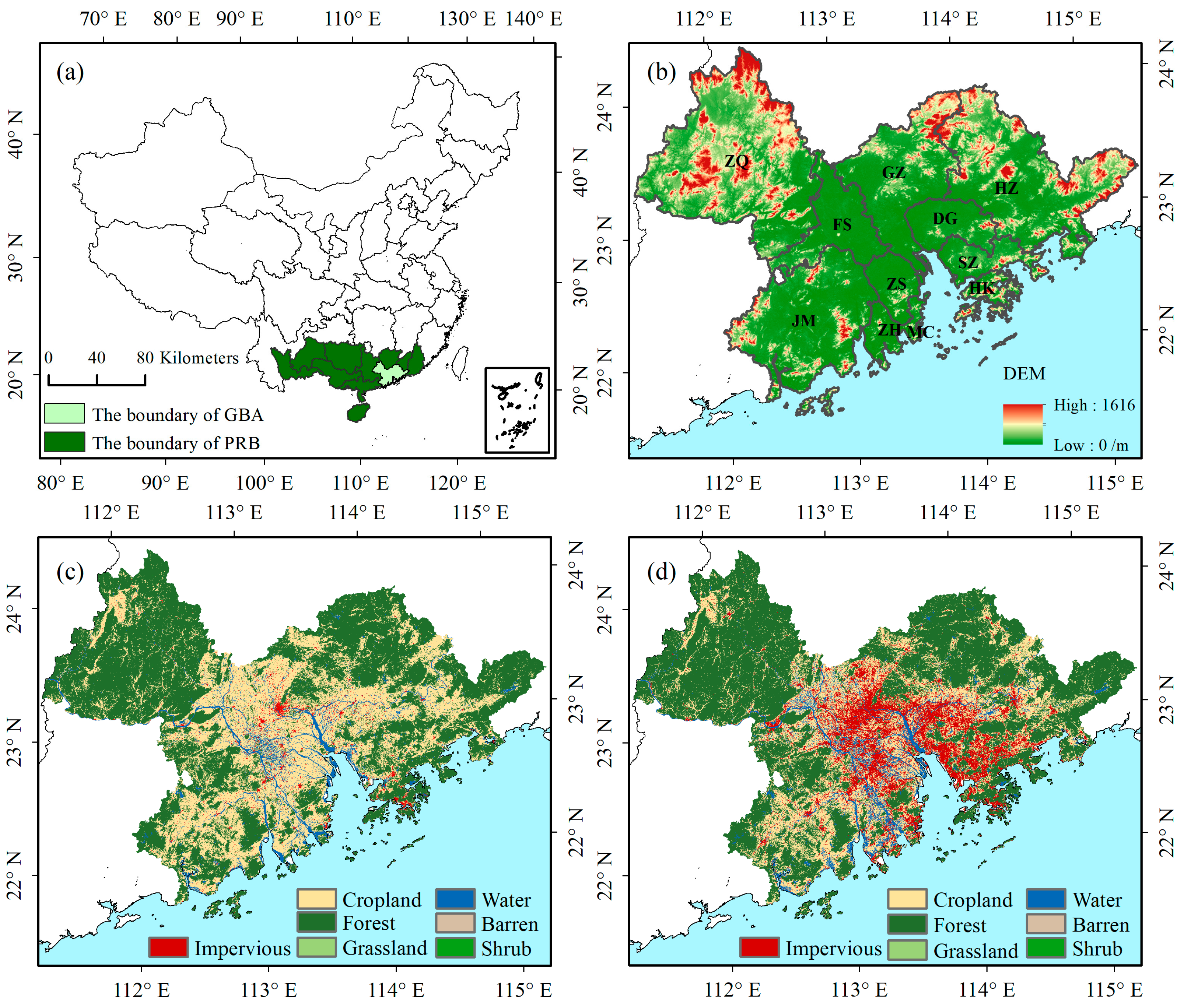
2.1. Study Area

The GBA is in the downstream of Pearl River Basin (PRB) (Figure 1a), and consists of Hongkong, Macao and nine cities (Guangzhou, Shenzhen, Zhuhai, Foshan, Huizhou, Dongguan, Zhongshan, Jiangmen, Zhaoqing) in Guangdong Province. The total area of GBA is approximately 56,000 km², the average elevation is about 130 m. Mountains encircle the GBA from the east, west, and north, and the central part is mainly a low altitude plain (Figure 1b). The GBA has a subtropical humid climate which is characterized by dramatic change of temperature and precipitation in summer and winter, with an annual mean temperature 21–23 °C [45], and an annual mean precipitation of 1300–2500 mm. As one of the most economically developed and urbanized regions in China, the GBA had over 70 million permanent residents in 2018, an increase of 1.5 times compared to the past two decades. And in 2018, the impervious surface was approximately 6731.665 km² (Figure 1d), marking a 6.71-fold increase from the 1002.756 km² recorded in 1985 (Figure 1c). Under such unique climate conditions and severe urbanization, GBA has suffered from typhoons and extreme rainstorms constantly, which have seriously threatened the safety of people’s lives and properties. For example, in August 2017, the strong typhoon “Hato” landed in GBA area, causing 9 deaths and economic losses of 11.922 billion yuan (http://smzt.gd.gov.cn/, accessed on 2 October 2022). Then in September 2018, another typhoon “Mangosteen” appeared in GBA, causing 4 deaths and economic losses of 4.249 billion yuan(http://smzt.gd.gov.cn/, accessed on 2 October 2022). And the 22 May 2020, a flooding event occurred, resulting in 5 deaths and the economic losses of approximately 2.8 billion RMB [46].

2.2. Data Source

2.2.1. Data for Urbanization Level Extraction

We acquired the land cover data for extracting urbanization levels from the annual China Land Cover Dataset (CLCD). from the annual China Land Cover Dataset (CLCD). This dataset was created utilizing Landsat datasets and the random forest classification method on the GEE platform, resulting in an overall accuracy of 80% [47,48]. The spatial resolution is 30 m, the temporal resolution is once a year, and only available in 1985 and 1990–2018. The land cover classification scheme comprises 9 types: cropland, forest, shrub, grassland, water, snow/ice, barren, impervious, wetland. The change of impervious surface is an important manifestation of urbanization, therefore, we take impervious surface as an indicator of urbanization. The pre-processing processes of CLCD, such as projection conversion, clipping, binarization, etc. are mainly carried out on ARCGIS 10.2. Besides, to capture the spatiotemporal characteristics of urbanization, the study employed a gridded vector layer with a 5-km resolution, and the impervious surface in 1985 and during 1990–2018 were assigned to each grid in the vector layer, and our study only analyzed spatial units that consist entirely of land. Finally, the urbanization level of each grid was defined as follow:

$$P_{i,j}=\frac{N_{i,j}·R}{S}\times 100\%$$

(1)

where P_i,j is the urbanization level of the grid i in year j. The parameter N_i,j represent the total number of impervious surface cells in grid i for year j, R is the resolution of CLCD, and S represents the l area of each grid (5 km × 5 km).

2.2.2. Data for Extreme Precipitation Detection

In this study, the China Meteorological Forcing Dataset (CMFD) [49] are obtained to detect the extreme precipitation for GBA. The dataset was created through fusion of remote sensing products, reanalysis dataset and in-situ observation data at meteorological stations [49,50]. It includes 7 near-surface meteorological elements of 2-m air temperature, surface pressure, specific humidity, 10-m wind speed, downward shortwave radiation, downward longwave radiation, and precipitation rate. The spatial resolution is 0.1° and the temporal resolution is three hours (http://data.tpdc.ac.cn/, accessed on 20 October 2022). It has an accuracy better than the existing satellite precipitation data and reanalysis data [29]. At present, it is only available for the period 1979–2018. Additionally, the dataset was resampled to a 5 km spatial resolution, consistent with the urbanization level data.

2.3. Methods

2.3.1. Extreme Precipitation Indices

We chose 11 Extreme Precipitation Indices (EPIs) (

Table 1. Definitions of EPIs.

Index	Descriptive Name	Definition	Units
PRCPTOT	Annual total precipitation	Annual total precipitation in wet days(RR ≥ 1 mm)	mm
NW	Wet days	Annual count of days when RR ≥ 1 mm	days
SDII	Simple daily intensity index	Average precipitation in wet days	mm/day
Rx1 Day	Maximum 1-day precipitation	Annual maximum 1-day precipitation	mm
Rx5 Day	Maximum 5-day precipitation	Annual maximum consecutive 5-day precipitation	mm
R95P	Very wet day precipitation	Annual total precipitation when RR ≥ 95th percentage	mm
R99P	Extreme wet day precipitation	Annual total precipitation when RR ≥ 99th percentage	mm
CWD	Consecutive wet days	Maximum number of consecutive wet days	days
R10 mm	Heavy precipitation days	Annual count of days when RR ≥ 10 mm	days
R20 mm	Very heavy precipitation days	Annual count of days when RR ≥ 20 mm	days
R50 mm	Extremely precipitation days	Annual count of days when RR ≥ 50 mm	days

) and the Annual Total Precipitation (ATP) to explore the spatiotemporal variations patterns of extreme precipitation in this study. The definition of each EPI is shown in Table 1, and the selected EPIs are derived from the Expert Team on Climate Change Detection and Indices (ETCCDI, http://etccdi.pacificclimate.org/, accessed on 20 August 2022), which have been extensively employed to examine the variation of extreme precipitation [51,52].

2.3.2. Theil-Sen Estimator and Mann-Kendall Trend Test

The Mann-Kendall [53] is a nonparametric statistical test method that doesn’t necessitate data to adhere to a particular distribution and is more resilient to outliers and missing values. The Theil-Sen Estimator method [54] is often integrated with the Mann-Kendall trend test to assess long-term trend patterns, both of them have been widely used in meteorology and hydrology [55,56].

For the time series variables x₁, x₂, x₃, …, x_n, the calculation formula of Theil-Sen Estimator is expressed as Equation (2). When β is great than 0, it indicates an increasing trend, while when β is less than 0, it signifies a decreasing Trend.

$$\beta =\mathit{mean}\left(\frac{x_i-x_j}{i-j}\right), \forall i>j$$

(2)

The mathematical formula of Mann-Kendall trend test is shown as Equations (3)–(6).

First, calculate the value of S:

$$S={\displaystyle \sum _{j-1}^{n-1}}{\displaystyle \sum _{i=j+1}^n}{f(x}_i-x_j)$$

(3)

$${ f(x}_i-x_j)=\left\{\begin{array}{c}-{1, x}_i-x_j<0\\ {0, x}_i-x_j=0\\ {1, x}_i-x_j>0\end{array} (1\le j< i \le n)\right.$$

(4)

Second, calculate the MK test statistic, Z, the variance VAR(S) of the statistics S is calculated using Equation (6). Where t_r is the number of ties for the rth value and g is the number of tied values.

$$Z=\left\{\begin{array}{c}\frac{S-1}{\sqrt{\mathrm{VAR}\left(S\right)}}, S> 0\\ 0, S=0\\ \frac{S+1}{\sqrt{\mathrm{VAR}\left(S\right)}}, S < 0\end{array}\right.$$

(5)

$$\mathrm{VAR}\left(S\right)=\frac{1}{18}\left[n\right(n-1\left)\right(2n+5)-{\displaystyle \sum _{r=1}^g}{t}_r{(t}_r-{1\left)\right(2t}_r+5\left)\right]$$

(6)

Third, the trend is considered significant, if Z is more than the significance levels such as $\alpha$ = 10% ($Z \ge Z_{1/\alpha }=\left|\pm 1.65\right|$), or $\alpha$ = 5% ($Z \ge Z_{1/\alpha }=\left|\pm 1.96\right|$). The positive values of Z indicate that the trend is positive while the negative values represent a negative trend in the time series.

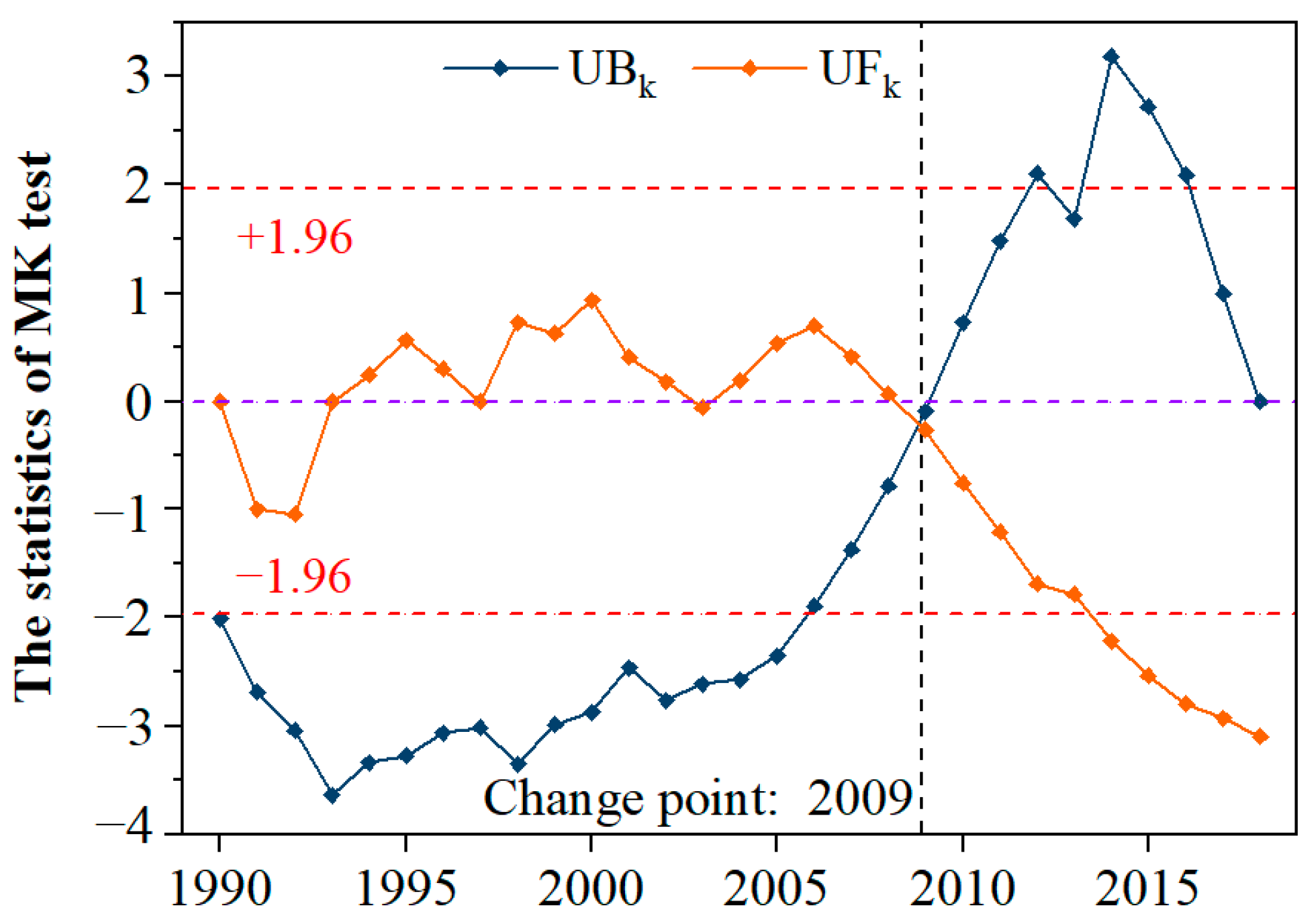
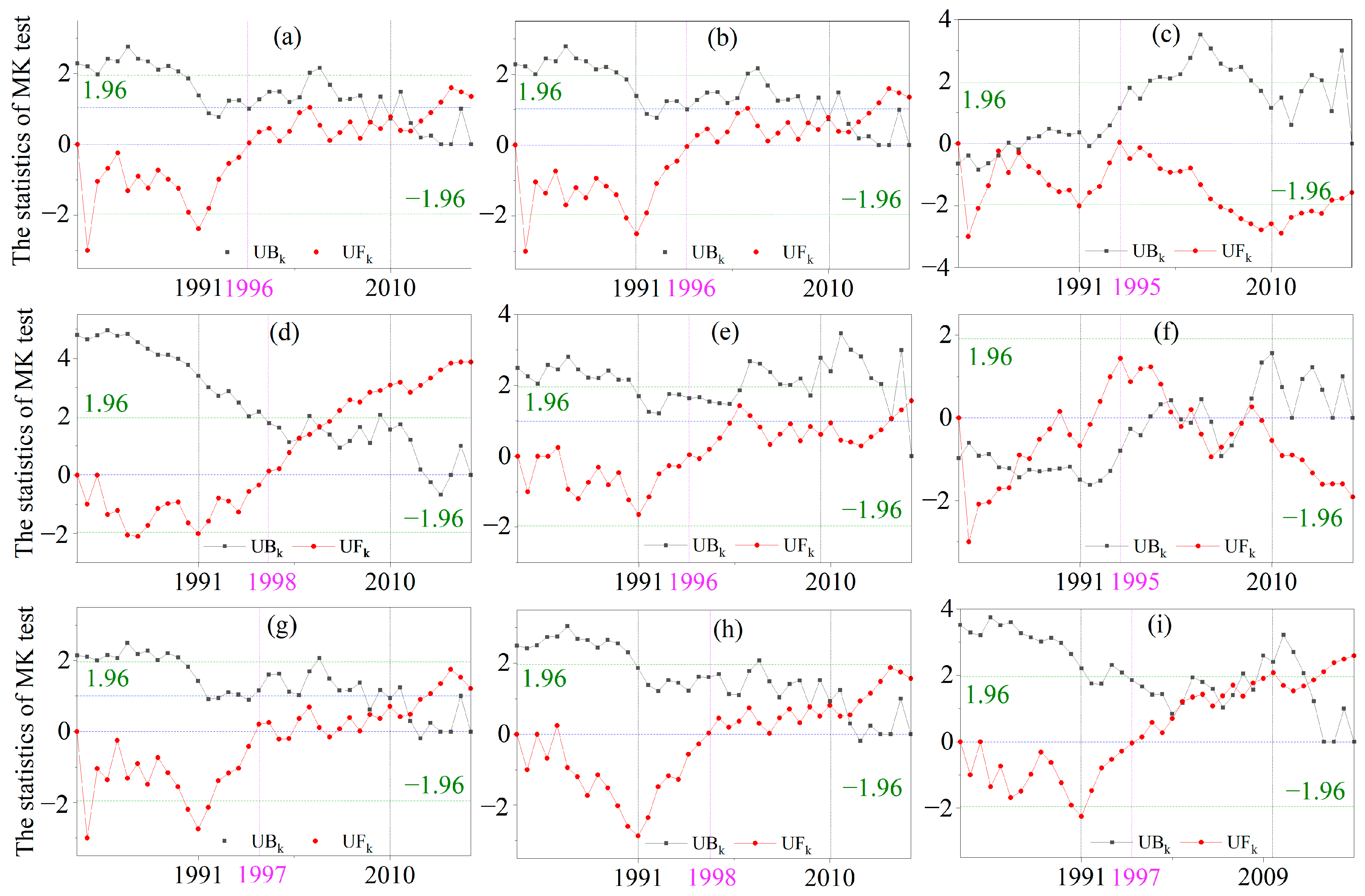
2.3.3. Mann-Kendall Mutation Test

Besides, the Mann-Kendall mutation test [57,58] was used in this paper to detect mutations in extreme precipitation time series. This test considers the relative values of all terms in the time series (x₁, x₂, x₃, …, x_n). It involves the following steps.

i. The test statistic S_k is obtained by Equation (7), and one order series, r_i, is conducted by comparing the magnitudes of x_j (j = 1, …, n) with x_k, (k = 1, …, j − 1), shown as Equation (8)

$$S_k={\displaystyle \sum _1^j}{r}_j$$

(7)

$$r_j=\left\{\begin{array}{c}{1, x}_j{>x}_k\\ 0, \mathrm{else}\end{array}\right.$$

(8)

ii. The Equations (9) and (10) are employed to calculate the mean and variance of the S_k:

$${\mathrm{E}(S}_k)=n(n-1)/4$$

(9)

$${\mathrm{VAR}(S}_k)=j(j-1\left)\right(2j+5)/72$$

(10)

iii. The successive UF_k values are calculated by Equation (11), and UB_k is the inverse order of UF_k.

$${\mathrm{UF}}_{\mathrm{k}}=\left[S_k-{\mathrm{E}(S}_k)\right]/\sqrt{{\mathrm{VAR}(S}_k)}$$

(11)

If the UF_k > 0 it indicates that the data exhibits an increasing trend, and vice versa. The ${\mathrm{UF}}_{\mathrm{k}}\ge {\mathrm{UF}\left(\mathrm{t}\right)}_{1-\mathsf{\alpha }/2}=\left|\pm 1.96\right|$, here, ${\mathrm{UF}\left(\mathrm{t}\right)}_{1-\mathsf{\alpha }/2}$ is the critical value of the standard normal distribution with a probability value greater than α/2, the data exhibit a significant increasing or decreasing trend. The intersection points of UF_k and UB_k exist between the credibility lines represent the potential mutations of the trend within a time series [59].

2.3.4. Bivariate Moran’s I

The Bivariate Moran’s I [60,61] was developed from the traditional spatial correlation analysis, global Bivariate Moran’s I and local Bivariate Moran’s I (bivariate LISA) were employed in our study. Global Bivariate Moran’s I can identify whether there is exist a spatial correlation relationship between two attributes across the entire area at a certain significance level, the values range is [−1, 1], negative values indicating negative spatial correlation, 0 implies no spatial correlation, while positive values represent positive spatial correlation, whereas local Bivariate Moran’s I can illustrate the relationship between two attributes in each space unit and its neighboring units.

We applied the following equations for calculation:

$${\mathrm{I}}_{\mathit{ab}}=\frac{n{{\displaystyle \sum }}_i^n{{\displaystyle \sum }}_{j\ne i}^n{w}_{i,j}{z}_i^a{z}_j^b}{(n-1){{\displaystyle \sum }}_i^n{{\displaystyle \sum }}_{j\ne i}^n{w}_{i,j}}$$

(12)

$${\mathrm{I}}_{\mathit{ab}}^{’}{=z}_i^a{{\displaystyle \sum }}_{j=1}^n{w}_{i,j}{z}_j^b$$

(13)

where ${\mathrm{I}}_{\mathit{ab}}$ and ${\mathrm{I}}_{\mathit{ab}}^{’}$ are the global and local Bivariate Moran’s I, respectively. n is the number of space units. $w_{i,j}$ is the spatial weights matrix for measuring spatial correlation between the space units i and j, which was generated based on geospatial weight method. $z_i^a$ represents the standardized value of attribute a for the geographical unit i. $z_j^b$ represents the standardized value of attribute b for the geographical unit j.

According to Equations (12) and (13), we used the Bivariate Moran’s I to analyze the relationship between EPIs trends and the rate of urbanization change, aiming to identify areas where precipitation is impacted by urbanization. The bivariate LISA [62] technique allows us to visualize spatial correlations through the creation of Moran scatter plots, cluster maps, and associated significance maps. The Moran scatter plots divide the spatial correlations into four types, represented by four quadrants. (a) Quadrant I: The High-High type (HH), which signifies the space unit with a high value of attribute a is surrounded by units with high value of attribute b. (b) Quadrant II: The High-Low type (HL), represents high values of attribute a is surrounded by low values of attribute b. (c) Quadrant III: The Low-High type (LH), denotes low values of attribute a is surrounded by high values of attribute b. (d) Quadrant IV: The Low-Low type (LL), indicates low values of attribute a is surrounded by low values of attribute b.

2.3.5. Spearman Correlation Coefficient

To understand the temporal correlation between extreme precipitation and urbanization, the Spearman Correlation Coefficient was applied. It is a nonparametric measure of rank correlation, which generally considered to be the Person’s linear correlation coefficient of the permuted variables, represented by Equation (14):

$$\rho =1-\frac{6{{\displaystyle \sum }}_i{d}_i^2}{{n(n}^2-1)}$$

(14)

where n is the number of data points of the two variable, d_i is the difference in ranks of the “ith” element. The correlation coefficient $\rho$ varies between −1 and 1, a $\rho$ value close to 1 means the higher values of one variable are associated with higher values of the other variable, whereas a $\rho$ value close to −1 suggest that higher values of one are associated with lower values of the other, and when a $\rho$ value close to 0, the association is weak between the two variables.

3. Results and Discussion

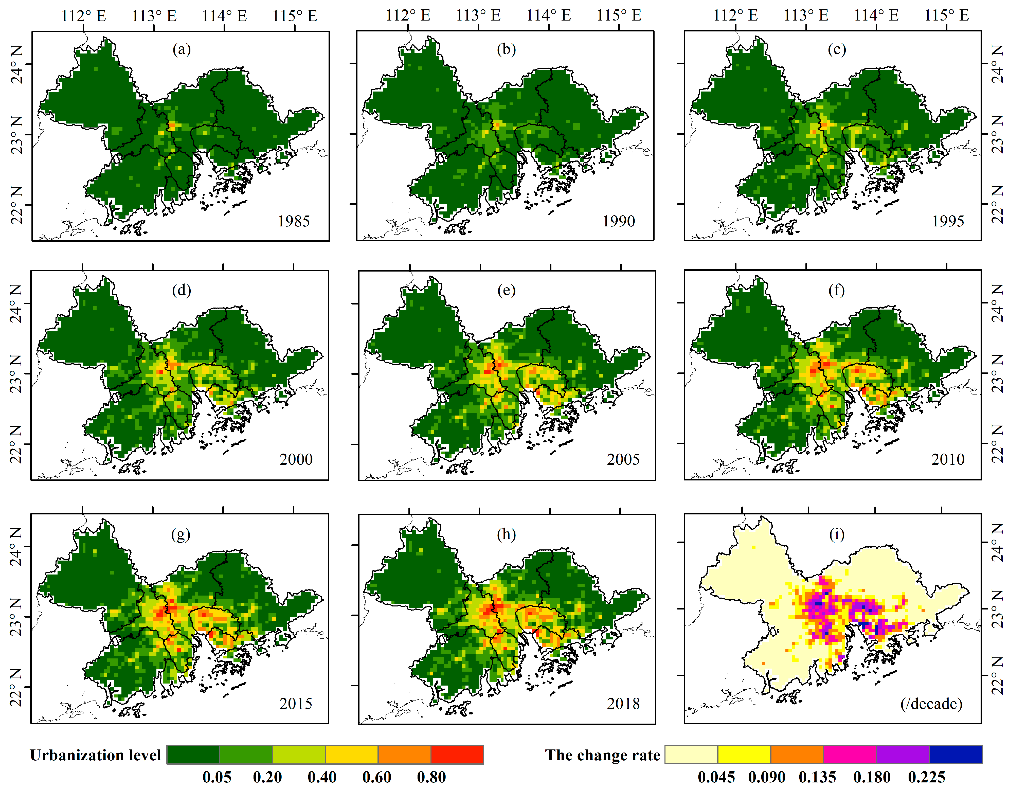
3.1. Urbanization Development in the GBA

Utilizing the CLCD dataset for the GBA in 1985 and the period from 1990 to 2018 we counted the change data of impervious surface area (Figure 2, the data for 1986–1989 was obtained by linear fitting), calculated the urbanization level in each 5 km grid according to Equation (1), the temporal and spatial changes of urbanization are shown in Figure 3 and

Table 2. The percentage of impervious surfaces in the GBA during the period of 1985–2018.

Citys	1985	1990	1995	2000	2005	2010	2015	2018	Change
Foshan	4.58%	5.36%	10.85%	16.74%	21.74%	26.84%	29.79%	31.23%	26.65%
Guangzhou	3.17%	3.64%	6.47%	9.68%	12.73%	15.47%	16.94%	17.88%	14.72%
Dongguan	3.77%	4.66%	12.36%	22.30%	32.44%	38.51%	41.47%	43.28%	39.51%
Zhongshan	3.07%	3.62%	8.68%	13.79%	19.61%	25.06%	28.38%	30.73%	27.66%
Shenzhen	2.55%	4.00%	12.00%	22.23%	30.31%	35.29%	37.35%	38.43%	35.88%
Huizhou	0.49%	0.62%	1.40%	2.11%	2.70%	3.56%	4.21%	4.69%	4.20%
Jiangmen	1.46%	1.77%	2.59%	3.52%	4.22%	5.04%	5.66%	6.08%	4.62%
Zhaoqing	0.69%	0.74%	0.95%	1.30%	1.52%	1.84%	2.11%	2.31%	1.62%
Zhuhai	1.76%	2.16%	5.02%	8.27%	10.67%	13.78%	16.51%	18.38%	16.62%
Hong Kong	6.47%	7.25%	9.13%	11.15%	12.08%	12.54%	12.86%	13.09%	6.62%
Macau	14.99%	15.95%	22.73%	26.96%	30.11%	32.82%	33.81%	34.38%	19.40%
GBA	1.80%	2.14%	4.14%	6.45%	8.49%	10.31%	11.41%	12.10%	10.30%

.

As illustrated in Figure 2a, the findings indicate that during the period of 1985–2018, the impervious surface area of the GBA exhibited a non-linear increasing trend, the impervious surface area increased from 1002.76 km² in 1985 to 6731.65 km² in 2018. According to the change of the annual increase area (Figure 2b), it is observed that since 1990, the annual increase area has demonstrated a fluctuating upward trajectory. As the urbanization process has slowed down, the annual increase impervious surface in urbanized area has gradually decreased, reaching an average of only 126.87 km² after 2010. Overall, the growth rate of impervious surfaces in the GBA showcased a pattern of initial increase followed by subsequent decrease between 1985 and 2018.

Figure 3a–h portrays the spatial distribution of urbanization levels at 5-year intervals. It is evident that the urbanization process in the GBA was notably pronounced from 1985 to 2018. Regions with elevated urbanization levels were primarily concentrated in Guangzhou, Foshan, Dongguan, Shenzhen, and Zhongshan. This conclusion is further supported by the change rate of urbanization levels depicted in Figure 3i, which highlights similar concentration patterns in the mentioned cities. Locations with change rates exceeding 9% are predominantly clustered in the southern areas of Guangzhou, Foshan, Dongguan, Shenzhen, and Zhongshan. Table 2 records the changes in impervious surface coverage in 11 cities within the GBA. Several key observations can be made from Table 2: Firstly, prior to 1990, there were relatively minor changes in impervious surface coverage, with an increase of only 0.34% in the GBA between 1985 and 1990. However, in the periods 1990–1995, 1995–2000, and 2000–2005, the rate of increase in impervious surface coverage notably accelerated, with increments of 2%, 2.31%, and 2.04%, respectively. Secondly, certain cities exhibited substantial changes in impervious surface coverage, with the order of increase being Dongguan, Shenzhen, Zhongshan, Foshan, Macau, Zhuhai, and Guangzhou, among others. Particularly noteworthy is that Dongguan and Shenzhen experienced an increase in impervious surface coverage exceeding 30%. In summary, from 1985 to 2018, the levels and change rates of urbanization in the GBA displayed distinct spatial and temporal characteristics. Notably, cities such as Dongguan, Shenzhen, Zhongshan, Foshan, and Guangzhou underwent concentrated and significant urbanization processes.

From the aforementioned analysis, it becomes evident that the urbanization process within the GBA does not exhibit a simple linear increase; rather, its pace of development demonstrates a pattern of initial growth followed by a decrease. To explore these distinct stages of urbanization within the GBA, we employ the MK method to detect mutations in the urbanization trajectory (as depicted in Figure 4). As shown in Figure 4, the urbanization pace within the GBA exhibited an ascending trajectory from 1993 to 2009, subsequently transitioning to a descending trend post-2008. Notably, after 2013, the urbanization pace underwent a substantial and statistically significant downward shift (Significance test passed at α = 0.05 level). The intersection point (2009) between the UF_k and UB_k curves falls within the range of −1.96 and +1.96 and given that UF_k surpassed the critical threshold of −1.96 in 2014, the intersection is statistically significant [54]. This intersection point is regarded as a mutation point in the urbanization development process. In conclusion, Combining the findings from Table 2 and Figure 4, the urbanization development process of the GBA can be categorized into three stages: Stage I (Pre-1990, absence of urbanization), Stage II (1991–2009, rapid urbanization), and Stage III (2010–2018, gradual urbanization). Additionally, the initial change point (1991) in urbanization development was identified through manual assessment.

3.2. Characteristics of Extreme Precipitation

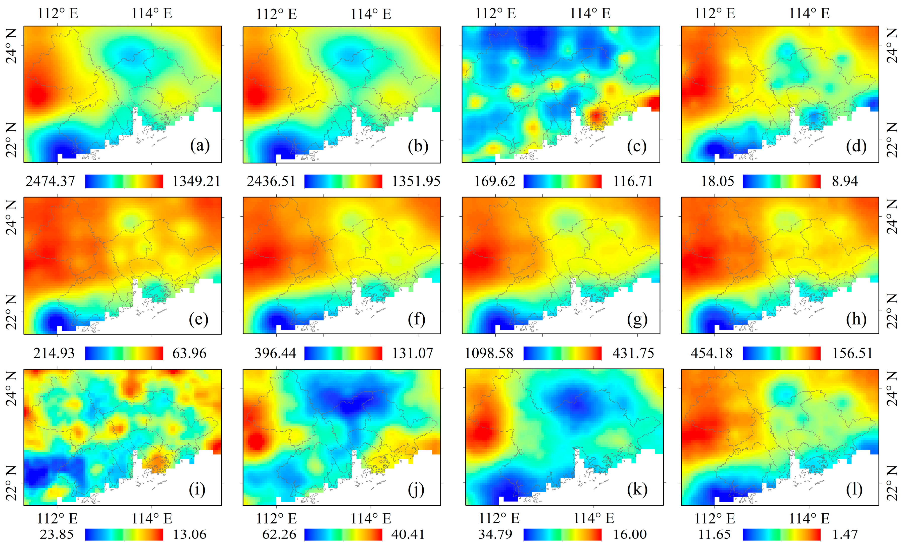
3.2.1. Spatio-Temporal Distribution of EPIs

Based on the CMFD dataset for the period 1979–2018, we calculated the ATP and 11 EPIs of the GBA. The spatial distributions of these 12 indicators are shown in Figure 5 (40-year average). Additionally, Figure 6 presents the values of 12 indicators during different urbanization development stages.

As depicted in Figure 5, the mean values of EPIs and ATP (except NW and CWD) show a consistent spatial pattern, with a gradual decrease from the coast towards the inland areas. Furthermore, there is a notable center of high extreme precipitation in the northern part of Guangzhou City, which is likely related to the urbanization process in the GBA. On the other hand, the spatial distribution analysis of NW and CWD reveals that although these two indices are influenced by ground station data and exhibit a bull’s-eye effect, certain highly urbanized areas (such as Guangzhou, Foshan, Shenzhen) have relatively lower NW and CWD values, indicating a higher likelihood of extreme rainfall occurrences in these regions.

To examine temporal changes in extreme precipitation within the GBA, this paper undertakes a concise analysis of extreme precipitation disparities across different urbanization stages in the GBA (Figure 6). The research findings indicate that, except for CWD and NW, the means and medians of the other indicators are higher in both urbanization stages II and III compared to stage I. Additionally, some indicators such as SDII, Rx1 day, R95P, R99P, R50 mm, and others exhibit relatively higher means and medians in urbanization stage III compared to stage II. Furthermore, guided by the analysis in Section 3.1, we classify Stage II as a phase of high-speed urbanization, Stage III as a period of gradual urbanization, and Stage I as a non-urbanization phase. As a result, we postulate that the urbanization process exerts a certain impact on the extreme precipitation patterns in the GBA, with varying degrees of influence across different urbanization stages. To quantitatively assess the effects of urbanization on extreme precipitation during distinct urbanization stages, the subsequent sections of this paper delve into relevant research.

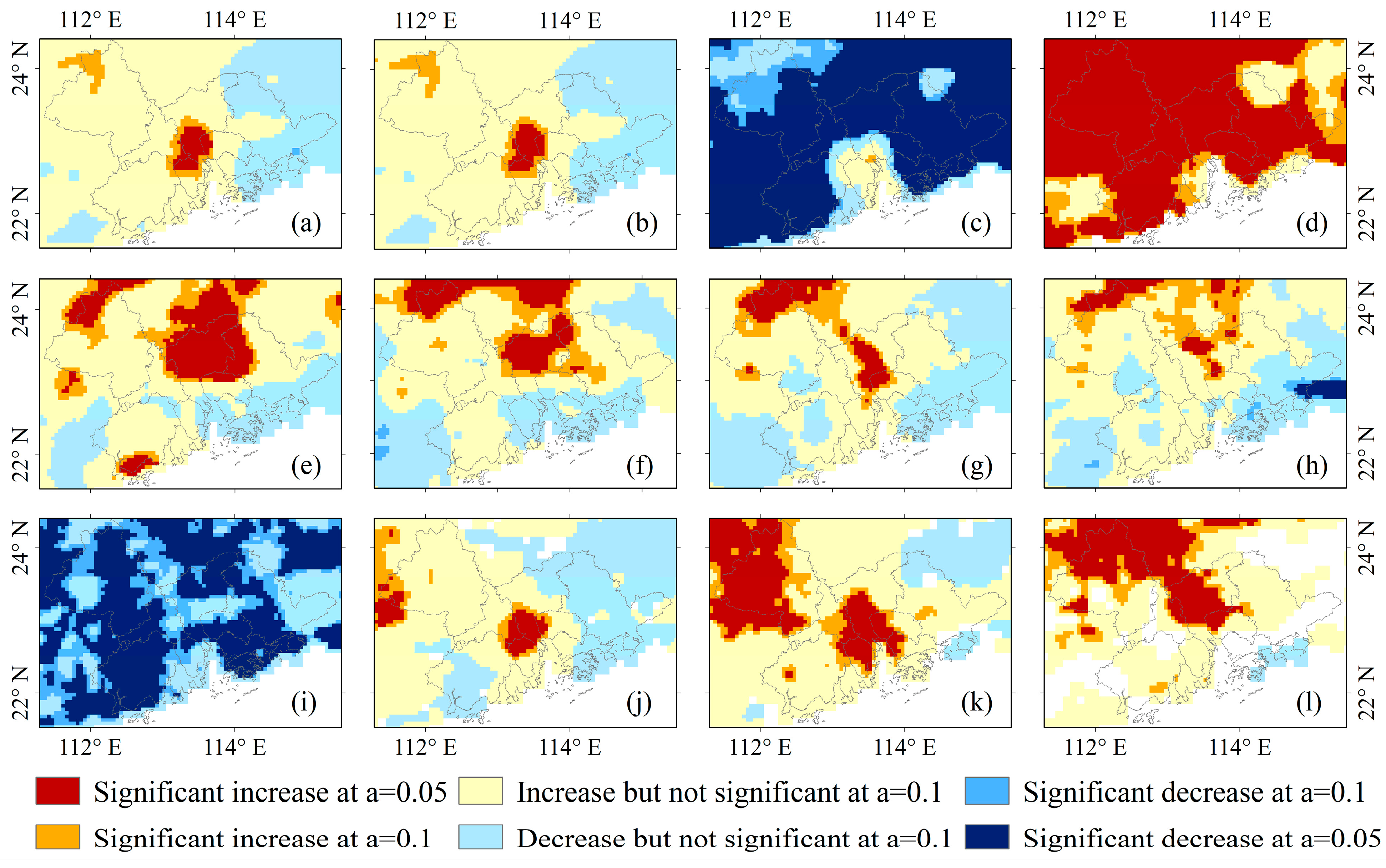
3.2.2. Spatio-Temporal Variations of EPIs

To explore the spatiotemporal variations of extreme precipitation in GBA from 1979 to 2018, we used Theil-Sen Estimator and Mann-Kendall test to calculate the trends (Figure 7) and significance (Figure 8) of 12 indices.

As illustrated in Figure 7 and Figure 8, the outcomes for most indicators (ATP, PRCPTOT, Rx1 day, Rx5 day, R95P, R99P, R10 mm, R20 mm, R50 mm) indicate a notable upward trend in extreme precipitation for cities such as Guangzhou, Foshan, Zhongshan, and Dongguan (statistically significant at the 0.05 level).And for cities like Zhaoqing, Huizhou, Jiangmen, Zhuhai, and Shenzhen, the trend in extreme precipitation exhibits either an insignificant increase or decrease (not statistically significant at the 0.1 level). Furthermore, the analysis results from Section 3.1 support the observation that the urbanization pace in Guangzhou, Foshan, Zhongshan, and Dongguan significantly surpasses that of other cities. Consequently, these findings provide further confirmation that the urbanization process in the Greater Bay Area indeed amplifies its occurrences of extreme precipitation.

Moreover, examining the trends in NW, CWD, and SDII, it becomes evident that a significant reduction in rainy days is observed across most regions of the GBA, coupled with a substantial increase in precipitation intensity. This phenomenon suggests that global climate change is also contributing to the enhancement of extreme precipitation within the GBA.

3.3. Association between EPIs and Urbanization

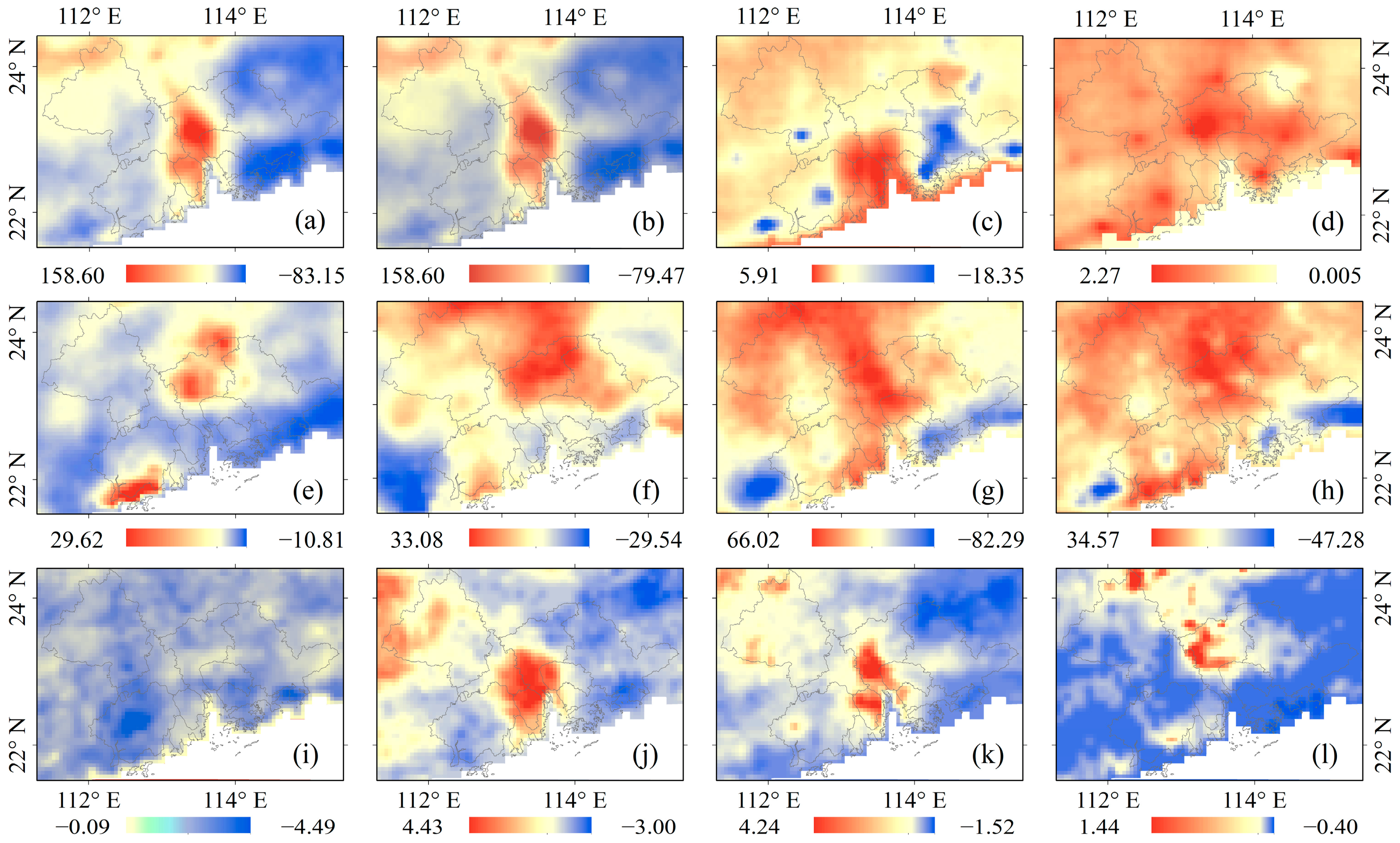
3.3.1. The Spatial Correlation between EPIs and Urbanization

From Section 3.2, we know that the extreme precipitation in highly urbanized cites of GBA (Guangzhou, Foshan, Zhongshan, Dongguan) exhibit a significant increase trend, therefore, to quantitatively express the spatial distribution relationship between the urbanization process and the change of extreme precipitation, this study calculated the Bivariate Moran’s I between the change rate of urbanization level and the trend of extreme precipitation from 1985 to 2018 in GBA, the results are shown in

Table 3. The global Bivariate Moran’s I between the trends of EPIs and change rate of urbanization.

Index	Moran’s I	p-Value	z-Value	Index	Moran’s I	p-Value	z-Value
ATP	0.335 *	<0.001	34.944	R95P	0.192 *	<0.001	20.721
PRCPTOT	0.328 *	<0.001	34.223	R99P	−0.014	0.05	−1.577
NW	0.259 *	<0.001	27.452	CWD	0.120 *	<0.001	12.926
SDII	0.038 *	<0.001	4.194	R10 mm	0.415 *	<0.001	41.726
Rx1 day	−0.024	0.004	−2.610	R20 mm	0.377 *	<0.001	38.121
Rx5 day	−0.122 *	<0.001	−13.018	R50 mm	0.087 *	<0.001	9.126

* Statistically significant at 1% level.

and Figure 8.

The global Bivariate Moran’s I values (Table 3) indicate significant positive spatial correlations (Moran’s I > 0 and p < 0.001) between the trends of indicators and the change rate of urbanization (such as PRCPTOT, NW, SDII, R95P, CWD, R10 mm, R20 mm, R50 mm). This suggests that areas with higher urbanization levels, such as Guangzhou, Foshan, Zhongshan, and Dongguan, exhibit a notable increase in extreme precipitation. However, the magnitude of positive correlation varied with extreme precipitation indices. Strong positive correlations exist between urbanization and R10 mm, R20 mm, ATP, PRCPTOT, NW, and R95P. Weaker positive correlations are found for R50 mm and SDII, while low negative correlations are observed between R99P, Rx1 day, Rx5 day, and urbanization., which means the spatial patterns of Rx1 day, Rx5 day and R99P may not be sensitive to the urbanization process in the GBA, As a result, other more sensitive indicators should be considered when studying extreme precipitation in the region.

The bivariate LISA map (Figure 9) illustrates four unique spatial aggregation patterns concerning the trend of 12 indicators and the change rate of urbanization. Notably, the HH clusters, characterized by high trends of 12 indicators and a high change rate of urbanization, are prominently concentrated within or on the periphery of urban areas. These clusters encompass portions of well-developed cities such as Guangzhou, Dongguan, Shenzhen, Zhuhai, Zhongshan, and Foshan. Conversely, LL clusters, signifying low trends of 12 indicators and a low change rate of urbanization, are dispersed across the northeastern and southwestern mountainous regions of the study area, including cities like Huizhou and Jiangmen. Another geographical cluster of LL is observed in Zhaoqing city. Similarly, HL clusters, denoting high trends of extreme precipitation indices and a low change rate of urbanization, are also clustered in the same mountainous areas, encompassing cities like Zhaoqing, Huizhou, and Jiangmen. These LL and HL clusters are primarily characterized by cropland and extensive natural areas, including forests, shrubbery, and grasslands. LH clusters, indicating low trends of extreme precipitation indices and a high change rate of urbanization, are situated around the HH clusters and are mainly concentrated in urban areas adjacent to the coastline, such as Shenzhen, Dongguan, Zhuhai, and Zhongshan. Due to the predominant influence of oceanic conditions on precipitation, the LH areas with high urbanization experience lower trends than the HH areas. Figure 10 illustrates the trends of the 12 indices across five cluster types in the LISA maps. Notably, the HH cluster exhibits higher trends compared to the other clusters (Insig, LL, LH, HL), implying that the variability of precipitation in urbanized regions surpasses that of other areas.

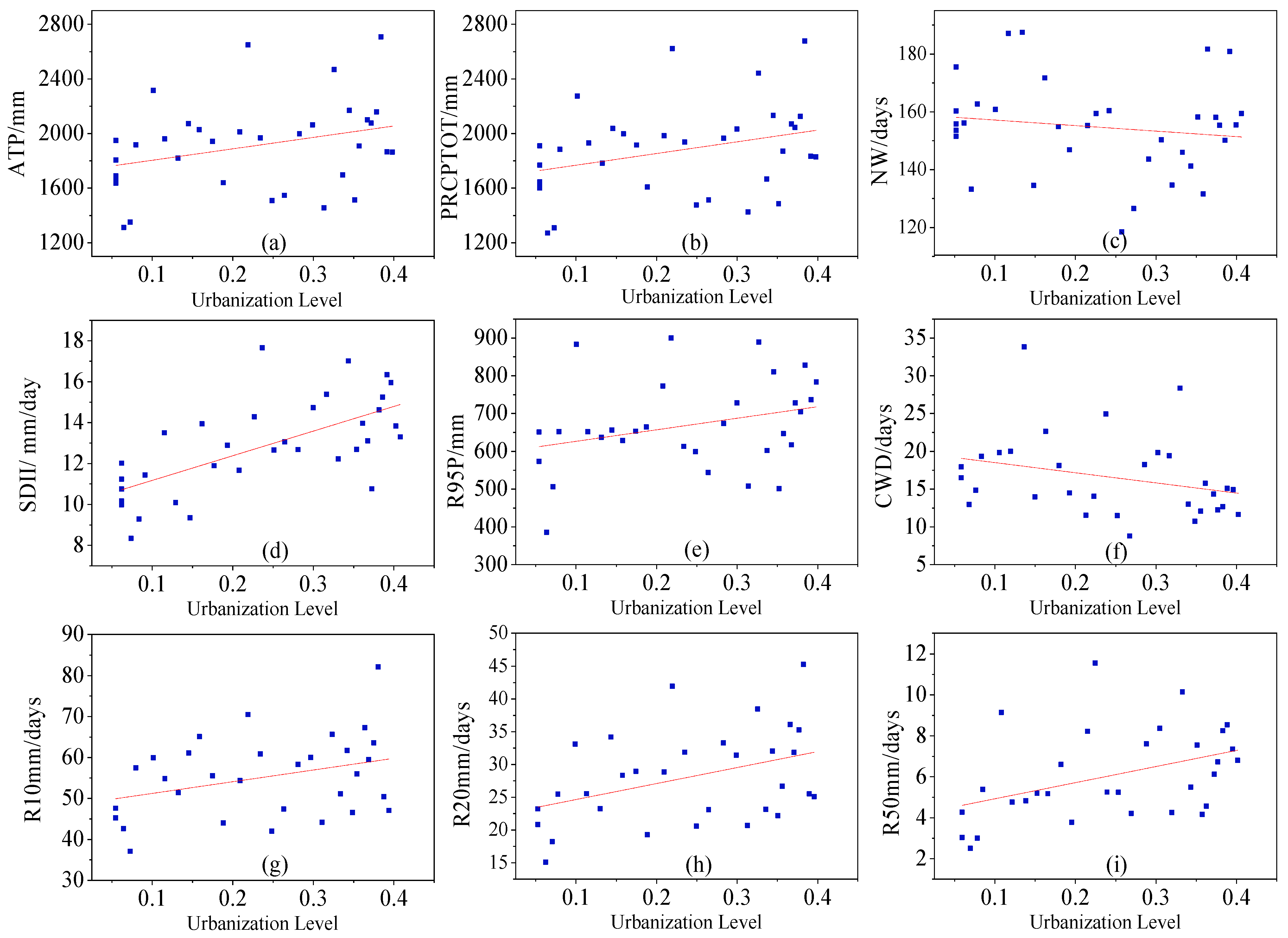
3.3.2. The Correlation between EPIs and Urbanization in Time Scale

To evaluate the relationship between urbanization and extreme precipitation over time, we focused on the High-High (HH) areas characterized by both a high urbanization change rate and a strong tendency of extreme precipitation (including ATP, PRCPTOT, NW, SDII, R95P, CWD, R10 mm, R20 mm, R50 mm). We generated scatter plots illustrating the relationship between EPIs and urbanization levels in these HH regions from 1985 to 2018 (Figure 11). Additionally, we calculated Spearman’s correlation coefficient between the average EPIs and the average urbanization level in the HH region for the period from 1985 to 2018 (

Table 4. Spearman Correlation between EPIs and urbanization during 1985–2018 in HH areas.

Indices	R-Value	p-Value	Indices	R-Value	p-Value
ATP	0.312 *	0.072	CWD	−0.289	0.113
PRCPTOT	0.319 *	0.066	R10 mm	0.336 *	0.064
NW	−0.148	0.402	R20 mm	0.401 **	0.025
SDII	0.661 **	<0.001	R50 mm	0.420 **	0.019
R95P	0.301 *	0.093

* Statistically significant at 0.1 level. ** Statistically significant at 0.05 level.

).

As depicted in Figure 10 and Figure 11, it’s evident that ATP, PRCPTOT, SDII, R95P, R10 mm, R20 mm, and R50 mm exhibit an upward trend as urbanization levels increase, whereas NW and CWD display a decline with rising urbanization levels. And the results of Spearman Correlation (

Table 5. The contributions of different urbanization stages to extreme precipitation.

Urbanization Process	Stage 1	Stage 2-1 (1991–2000)	Stage 2-2 (2001–2009)	Stage 2 (1991–2009)	Stage 3 (2010–2018)	Increase (Stage 2 to Stage 3)
ATP	/	49.14%	51.95%	50.58%	56.13%	5.55%
PRCPTOT	/	50.70%	53.23%	52.00%	57.29%	5.29%
SDII	/	12.30%	13.42%	12.84%	22.28%	9.44%
R95P	/	38.90%	40.47%	39.55%	53.10%	13.55%
R10 mm	/	65.07%	60.42%	62.89%	78.06%	15.17%
R20 mm	/	39.93%	35.42%	37.63%	44.36%	6.73%
R50 mm	/	11.72%	23.49%	15.39%	20.63%	5.24%

) also represented that the EPIs (except NW and CWD, the R of other indicators are all greater than 0.30) are positively temporally correlated with the urbanization. The strongest correlation was found between SDII and urbanization (R = 0.661), followed by R50 mm (R = 0.420) and R20 mm (R = 0.401), these three correlation coefficients all statistically significant at 0.05 level. Correlations between R10 mm, PRCPTOT, ATP, and R95P with urbanization are significant at the 0.1 level (R ranging from 0.301 to 0.336). While the correlation coefficients between CWD and urbanization (R = −0.289), NW and urbanization (R = −0.148) are less than 0, it shows that they are negatively correlated with the urbanization, but the correlations is not statistically significant.

3.4. Discussion

In this paper, our study examined the evolving patterns of urbanization and extreme precipitation in the GBA from 1985 to 2018 and explored the spatial and temporal correlations between urbanization and extreme precipitation changes. The study revealed that extreme precipitation in the GBA exhibited a consistent upward trend, particularly in urbanized areas and their surrounding regions. (Section 3.2). The research results clearly indicate that there is a pronounced spatiotemporal correlation between the urbanization process in the Greater Bay Area (GBA) and the trends in extreme precipitation. (Section 3.3). And these results are in accordance with previous studies [41,45], which analyzed precipitation differences between urban and rural areas using rain gauge data from meteorological stations. Similarly, Wai et al. [30] and Li et al. [31] employed the WRF-SLUCM model to demonstrate that urbanization in the GBA indeed intensified precipitation. Our study offers the benefits of mapping the enduring spatial and temporal alterations in extreme precipitation and urbanization, it can explore the impact of urbanization on extreme precipitation from a continuous spatio-temporal scale. However, several issues remain to be addressed. Firstly, how does extreme precipitation change alongside GBA urbanization? To address this issue, this paper uses the MK mutation test method to try to obtain some relevant information, the results are shown in Section 3.4.1. Secondly, how can the urbanization contribution to extreme precipitation be quantified across different urbanization stages? Addressing this, Section 3.4.2 further analyzes statistical values of extreme precipitation under distinct urbanization processes, quantifying the extent to which urbanization contributes to extreme precipitation in GBA.

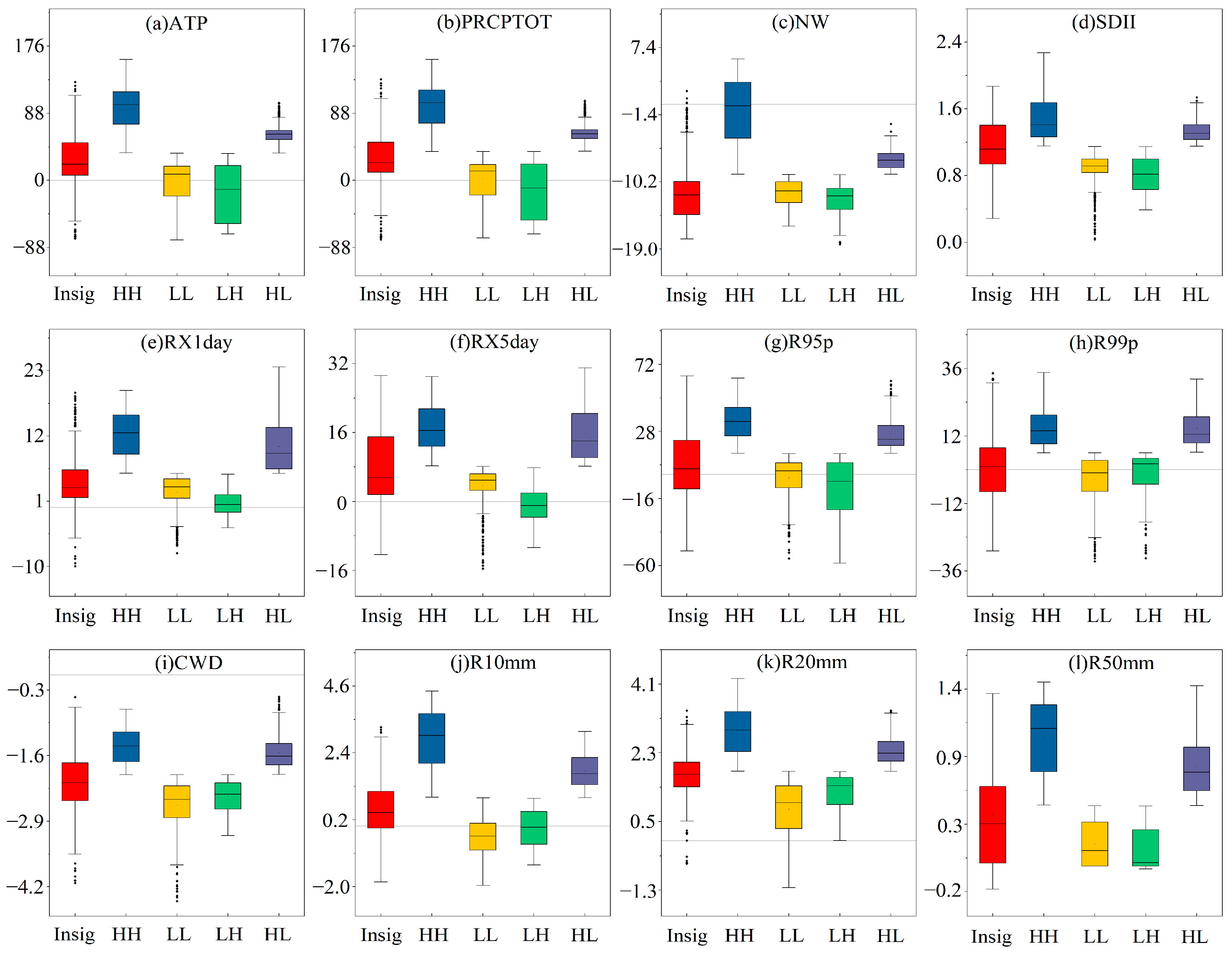
3.4.1. Changes of Extreme Precipitation at Different Urbanization Stages

To investigate how extreme precipitation has evolved in the highly urbanized areas of the GBA (HH) at different stages of urbanization, we conducted a 40-year analysis from 1979 to 2018 using the Mann-Kendall (MK) trend test, and the findings are illustrated in Figure 12.

Figure 12 presents the results of MK test for the average EPIs in HH areas during the period of 1985–2018. The results reveal diverse trends in extreme precipitation during various urbanization stages, which indicates that different urbanization stages have different impacts on extreme precipitation. First, the UF_k curves of all EPIs were less than zero in stage I (Slow urbanization), this suggests that extreme precipitation shows a decreasing trend due to the other environmental factors such as monsoon climate [63], circulation [64] before the urbanization process. Second, in the stage II (Rapid urbanization), except for NW (Figure 12c) and CWD (Figure 12f), the UF_k curves of other EPIs all shifted from a downward trend (UF_k < 0) to an upward trend (UF_k > 0), and the time nodes for trend changes are all between 1996–1998 (The purple line in Figure 10). Before the transition time nodes, those EPIs mainly show a downward trend, and after the transition time node, those EPIs mainly show an upward trend, but the UF_k curves of SDII and R50 mm are obviously different from the UFK curves of ATP, PRCPTOT, R95P, R10 mm and R20 mm, the two curves eventually exceeded the critical line of 1.96 (Significantly increased at 0.05 level) and the UF_k curves of ATP, PRCPTOT, R95P, R10 mm and R20 mm only change between [0, 1]. Third, in the stage III (Stable stage), except for NW (Figure 12c) and CWD (Figure 12f), the UF_k curves of other EPIs rise further and all greater than that in the stage I (Slow urbanization) and stage II (Rapid urbanization), it means that in the third stage, extreme precipitation has further intensified.

3.4.2. Influence of Urbanization on Extreme Precipitation at Different Urbanization Stages

The above research results show that extreme precipitation changes have a high temporal and spatial correlation with the urbanization process, and different urbanization stages have different effects on extreme precipitation. Extreme precipitation is influenced not only by the urbanization process but also by climate change. To quantitatively assess the influence of different urbanization stages on extreme precipitation in the GBA, based on the research results in Section 3.2 and Section 3.3, this chapter selects the HH areas in the GBA where there is a strong correlation between extreme precipitation trends and urbanization change rate, s and the HL areas which are either not influenced by urbanization or are affected to a lesser extent, to study the impact of urbanization on extreme precipitation in GBA. The change of extreme precipitation in HL areas can be attributed to climate change, and the extreme precipitation in HH region experiences the influence of both urbanization and climate change. And the two regions are under the same regional climate background, so the influence of climate change on extreme precipitation in the two regions can be regarded as equivalent. Therefore, we can obtain the difference in extreme precipitation between the HH region and the HL region, remove the impact of regional climate change on extreme precipitation, thus evaluate the impact of urbanization on extreme precipitation.

Before urbanization (Stage 1 in Section 3.1), the extreme precipitation in the highly urbanized area (HH) is labeled as EPI_u1, and the suburban area (HL) is EPI_r1. After urbanization (Stage 2 and Stage 3 in Section 3.1), extreme precipitation in the highly urbanized areas (HH) can be expressed as EPI_u2 = ${\mathrm{EPI}}_{\mathrm{u}1}+\Delta {\mathrm{P}}_{\mathrm{urbanization}}+\Delta {\mathrm{P}}_{\mathrm{climate}}$, and for suburban area (HL) as EPI_r2 = ${\mathrm{EPI}}_{\mathrm{r}1}+\Delta {\mathrm{P}}_{\mathrm{climate}}$. Then we can calculate the amount of precipitation influenced by urbanization as $\Delta {\mathrm{P}}_{\mathrm{urbanization}}{=\mathrm{EPI}}_{\mathrm{u}2}-{\mathrm{EPI}}_{\mathrm{u}1}-\left({\mathrm{EPI}}_{\mathrm{r}2}-{\mathrm{EPI}}_{\mathrm{r}1}\right)$, the contribution of urbanization is denoted as $\rho =\left|\frac{\Delta {\mathrm{P}}_{\mathrm{urbanization}}}{{\mathrm{EPI}}_{\mathrm{u}2}-{\mathrm{EPI}}_{\mathrm{u}1}}\right|\times 100\%$. To assess the impact of urbanization on extreme precipitation accurately, we selected seven sensitive indicators, ATP, PRCPTOT, SDII, R95P, R10 mm, R20 mm and R50 mm, which are positively correlated with the urbanization process, and according to three stages (Section 3.1, no urbanization, rapid urbanization, and slow urbanization) to explore the impact of urbanization on extreme precipitation of GBA, the results are shown in Table 5.

Based on the findings presented in Table 5, it is evident that the influence of urbanization on extreme precipitation in the highly urbanized areas of the GBA (HH) has become increasingly pronounced, this effect is particularly notable during the later phases of urbanization, where urbanization accounted for a substantial 20% to 80% of the escalation in extreme precipitation. During the initial phase of rapid urbanization (Stage2-1), the contribution of urbanization to ATP increase was 49.14%, and regarding the other six EPIs, the contribution from high to low were as follows: 65.07% (R10 mm), 50.70% (PRCPTOT), 39.93% (R20 mm), 38.90% (R95P), 12.30% (SDII), and 11.72% (R50 mm). During this stage of urbanization, the largest contribution was observed for the R10 mm, while the smallest contributions were seen for the rainfall intensity indicator SDII and the indicator for days with rainfall exceeding 50 mm (R50 mm). In the later stage of rapid urbanization (Stage2-2), both ATP and various extreme precipitation indicators demonstrate a further increase in the contribution of the urbanization process to extreme precipitation (except for slight decreases in the R10 mm and R20 mm indicators), and the extent to which extreme precipitation indicators R10 mm, PRCPTOT, R95P, and ATP are influenced by urbanization exceeds 40%. During the stage of slow urbanization (2010–2018), the impact of the urbanization process on extreme precipitation further intensifies. Among them, the R10 mm indicator demonstrates a contribution of urbanization to extreme precipitation exceeding 78.06% (an increase of 15.17% compared to Stage 2). The PRCPTOT, R95P, and ATP indicators also reach levels of over 53%, while the influence of urbanization on the SDII and R50 mm indicators rises to more than 20%.

4. Conclusions

In conclusion, this study provides a comprehensive analysis of the urbanization development and the spatiotemporal evolution of extreme precipitation in the GBA from 1985 to 2018, revealing a close relationship between urbanization and extreme precipitation. Specifically, the main conclusions drawn from this study include.

(1) During the period from 1985 to 2018, the impervious surface area in the GBA exhibited a nonlinear growth trend, the impervious surface area increased from 1002.76 km² in 1985 to 6731.65 km² in 2018. Regions with elevated urbanization levels were primarily concentrated in Guangzhou, Foshan, Dongguan, Shenzhen, and Zhongshan. The urbanization development of the GBA can be categorized into three stages: Stage I (pre-1990, no urbanization), Stage II (1991–2009, rapid urbanization), and Stage III (2010–2018, slow urbanization).

(2) Compared to cities with lower levels of urbanization, the highly urbanized areas within the GBA, including Guangzhou, Foshan, Zhongshan, and Dongguan, demonstrated a significant upward trend in extreme precipitation. On the other hand, the GBA also saw a reduction in the count of rainy days coupled with an elevation in precipitation intensity, indicating that global climate change might also contribute to the intensification of extreme precipitation in the GBA.

(3) The trends of ATP, PRCPTOT, SDII, R95P, R10 mm, R20 mm, and R50 mm exhibit significant positive spatiotemporal correlations with the change rate of urbanization in GBA. Specifically, R10 mm displays the highest spatial correlation at 0.415, while SDII demonstrates the highest temporal correlation at 0.661. Consequently, this study focused on these seven indicators, which are notably responsive to the urbanization process, for assessing the influence of urbanization on extreme precipitation.

(4) The influence of urbanization on extreme precipitation in highly urbanized regions of the GBA is progressively intensifying along with urban development. During the stage of slow urbanization, urbanization contributes to a 56.13% increase in ATP in the GBA, and its contribution to the increase in extreme precipitation ranges from 20% to 80%. Notably, R10 mm exhibited the highest contribution at 78.06%, while even R50 mm demonstrated a contribution exceeding 20%.

References

1. Abbott, B.W.; Bishop, K.; Zarnetske, J.P.; Minaudo, C.; Chapin, F.; Krause, S.; Hannah, D.M.; Conner, L.; Ellison, D.; Godsey, S.E. Human domination of the global water cycle absent from depictions and perceptions. Nat. Geosci. 2021, 12, 533–540. [Google Scholar] [CrossRef]
2. Douville, H.; Raghavan, K.; Renwick, J.; Allan, R.P.; Arias, P.A.; Barlow, M.; Cerezo-Mota, R.; Cherchi, A.; Gan, T.; Gergis, J.; et al. Water cycle changes. In Climate Change 2021: The Physical Science Basis. Contribution of Working Group I to 45 the Sixth Assessment Report of the Intergovernmental Panel on Climate Change; Cambridge University Press: Cambridge, UK, 2021. [Google Scholar]
3. Ingram, W. Increases all round. Nat. Clim. Chang. 2016, 6, 443–444. [Google Scholar] [CrossRef]
4. Najibi, N.; Devineni, N. Recent trends in the frequency and duration of global floods. Earth Syst. Dynam. 2018, 9, 757–783. [Google Scholar] [CrossRef]
5. Zhang, W.; Villarini, G.; Vecchi, G.A.; Smith, J.A. Urbanization exacerbated the rainfall and flooding caused by hurricane Harvey in Houston. Nature 2018, 563, 384–388. [Google Scholar] [CrossRef]
6. Su, B.; Huang, J.; Fischer, T.; Wang, Y.; Kundzewicz, Z.W.; Zhai, J.; Sun, H.; Wang, A.; Zeng, X.; Wang, G. Drought losses in China might double between the 1.5 C and 2.0 C warming. Proc. Natl. Acad. Sci. USA 2018, 115, 10600–10605. [Google Scholar] [CrossRef] [PubMed]
7. Douris, J.; Kim, G. The Atlas of Mortality and Economic Losses from Weather, Climate and Water Extremes (1970–2019); WMO: Geneva, Switzerland, 2021. [Google Scholar]
8. Tellman, B.; Sullivan, J.; Kuhn, C.; Kettner, A.; Doyle, C.; Brakenridge, G.; Erickson, T.; Slayback, D. Satellite imaging reveals increased proportion of population exposed to floods. Nature 2021, 596, 80–86. [Google Scholar] [CrossRef] [PubMed]
9. Liu, B.; Chen, S.; Tan, X.; Chen, X. Response of precipitation to extensive urbanization over the Pearl River Delta metropolitan region. Environ. Earth Sci. 2021, 80, 9. [Google Scholar] [CrossRef]
10. Donat, M.G.; Lowry, A.L.; Alexander, L.V.; O’Gorman, P.A.; Maher, N. More extreme precipitation in the world’s dry and wet regions. Nat. Clim. Chang. 2016, 6, 508–513. [Google Scholar] [CrossRef]
11. Eyring, V.; Gillett, N.P.; Achutarao, K.; Barimalala, R.; Barreiro Parrillo, M.; Bellouin, N.; Cassou, C.; Durack, P.J.; Kosaka, Y.; McGregor, S.; et al. Climate Change 2021: The Physical Science Basis. Contribution of Working Group I to the Sixth Assessment Report of the Intergovernmental Panel on Climate Change; IPCC Sixth Assessment Report; Cambridge University Press: Cambridge, UK; New York, NY, USA, 2021. [Google Scholar]
12. Haas, J.; Ban, Y. Urban growth and environmental impacts in jing-jin-ji, the yangtze, river delta and the pearl river delta. Int. J. Appl. Earth Obs. Geoinf. 2014, 30, 42–55. [Google Scholar] [CrossRef]
13. Seto, K.C.; Guneralp, B.; Hutyra, L.R. Global forecasts of urban expansion to 2030 and direct impacts on biodiversity and carbon pools. Proc. Natl. Acad. Sci. USA 2012, 109, 16083–16088. [Google Scholar] [CrossRef]
14. Wang, Y.; Xie, X.; Liang, S.; Zhu, B.; Yao, Y.; Meng, S.; Lu, C. Quantifying the response of potential flooding risk to urban growth in Beijing. Sci. Total Environ. 2019, 705, 135868. [Google Scholar] [CrossRef] [PubMed]
15. Du, H.; Wang, D.; Wang, Y.; Zhao, X.; Qin, F.; Jiang, H.; Cai, Y. Influences of land cover types, meteorological conditions, anthropogenic heat and urban area on surface urban heat island in the Yangtze River Delta Urban Agglomeration. Sci. Total Environ. 2016, 571, 461–470. [Google Scholar] [CrossRef] [PubMed]
16. Kennedy, C.A.; Stewart, I.; Facchini, A.; Cersosimo, I.; Mele, R.; Chen, B.; Uda, M.; Kansal, A.; Chiu, A.; Kim, K.-G. Energy and material flows of megacities. Proc. Natl. Acad. Sci. USA 2015, 112, 5985–5990. [Google Scholar] [CrossRef]
17. Pielke, R.A., Sr. Land use and climate change. Science 2005, 310, 1625–1626. [Google Scholar] [CrossRef] [PubMed]
18. Shepherd, J.M.; Burian, S.J. Detection of urban-induced rainfall anomalies in a major coastal city. Earth Interact. 2003, 7, 1–17. [Google Scholar] [CrossRef]
19. Yao, R.; Zhang, S.; Sun, P.; Dai, Q.; Yang, Q. Estimating the impact of urbanization on non-stationary models of extreme precipitation events in the Yangtze River Delta metropolitan region. Weather Clim. Extremes 2022, 36, 100445. [Google Scholar] [CrossRef]
20. Huff, F.A.; Changnon, S., Jr. Climatological assessment of urban effects on precipitation at St. Louis. J. Appl. Meteorol. Climatol. 1972, 11, 823–842. [Google Scholar] [CrossRef]
21. Kong, F.; Wang, Y.; Fang, J.; Lu, L. Spatial Pattern of Summer Extreme Precipitation and Its Response to Urbanization in China (1961–2010). Resour. Environ. Yangtze Basin. 2018, 27, 996–1010. (In Chinese) [Google Scholar]
22. Deng, Z.; Wang, Z.; Wu, X.; Lai, C.; Liu, W. Effect difference of climate change and urbanization on extreme precipitation over theGuangdong-Hong Kong-Macao Greater Bay Area. Atmos. Res. 2023, 282, 106514. [Google Scholar] [CrossRef]
23. Kalnay, E.; Cai, M. Impact of urbanization and land-use change on climate. Nature 2003, 423, 528–531. [Google Scholar] [CrossRef]
24. Pathirana, A.; Denekew, H.B.; Veerbeek, W.; Zevenbergen, C.; Banda, A.T. Impact of urban growth-driven landuse change on microclimate and extreme precipitation—A sensitivity study. Atmos. Res. 2014, 138, 59–72. [Google Scholar] [CrossRef]
25. Paul, S.; Ghosh, S.; Mathew, M.; Devanand, A.; Karmakar, S.; Niyogi, D. Increased spatial variability and intensification of extreme monsoon rainfall due to urbanization. Sci. Rep. 2018, 8, 3918. [Google Scholar] [CrossRef] [PubMed]
26. Zhao, Y.; Tao, J.; Li, H.; Zuo, Q.; He, Y.; Du, W. Influence ofTeleconnection Factors on ExtremePrecipitation in Henan Provinceunder Urbanization. Water 2023, 15, 3264. [Google Scholar] [CrossRef]
27. Zhao, N.; Jiao, Y.; Ma, T.; Zhao, M.; Fan, Z.; Yin, X.; Liu, Y.; Yue, T. Estimating the effect of urbanization on extreme climate events in the Beijing-Tianjin-Hebei region, China. Sci. Total Environ. 2019, 688, 1005–1015. [Google Scholar] [CrossRef] [PubMed]
28. Mote, T.L.; Lacke, M.C.; Shepherd, J.M. Radar signatures of the urban effect on precipitation distribution: A case study for Atlanta, Georgia. Geophys. Res. Lett. 2007, 34, L20710-n. [Google Scholar] [CrossRef]
29. Zhao, Y.; Xia, J.; Xu, Z.; Zou, L.; Qiao, Y.; Li, P. Impact of urban expansion on rain island effect in Jinan city, north China. Remote Sens. 2021, 13, 2989. [Google Scholar] [CrossRef]
30. Wai, K.; Wang, X.; Lin, T.; Wong, M.S.; Zeng, S.; He, N.; Ng, E.; Lau, K.; Wang, D. Observational evidence of a long-term increase in precipitation due to urbanization effects and its implications for sustainable urban living. Sci. Total Environ. 2017, 599, 647–654. [Google Scholar] [CrossRef]
31. Li, Y.; Wang, W.; Chang, M.; Wang, X. Impacts of urbanization on extreme precipitation in the Guangdong-Hong Kong-Macau Greater Bay Area. Urban Clim. 2021, 38, 100904. [Google Scholar] [CrossRef]
32. Kusaka, H.; Kondo, H.; Kikegawa, Y.; Kimura, F. A simple single-layer urban canopy model for atmospheric models: Comparison with multi-layer and slab models. Bound.-Lay. Meteorol. 2001, 101, 329–358. [Google Scholar] [CrossRef]
33. Kusaka, H.; Kimura, F. Coupling a single-layer urban canopy model with a simple atmospheric model: Impact on urban heat island simulation for an idealized case. J. Meteorol. Soc. Jpn. Ser. II 2004, 82, 67–80. [Google Scholar] [CrossRef]
34. Wyszogrodzki, A.A.; Miao, S.; Chen, F. Evaluation of the coupling between mesoscale-WRF and LES-ULAG models for simulating fine-scale urban dispersion. Atmos. Res. 2012, 118, 324–345. [Google Scholar] [CrossRef]
35. Hu, Q.; Zhang, J.; Wang, Y.; Huang, Y.; Liu, Y.; Li, L. A review of urbanization impact on precipitation. Adv. Water Sci. 2018, 29, 138–150. (In Chinese) [Google Scholar]
36. Yang, L.; Tian, F.; Sun, T.; Ni, G. Advances in research of urban modification on rainfall over Beijing metropolitan region. J. Hydrol. Eng. 2015, 34, 37–44. (In Chinese) [Google Scholar]
37. Beniston, M.; Stephenson, D.B.; Christensen, O.B.; Ferro, C.A.; Frei, C.; Goyette, S.; Halsnaes, K.; Holt, T.; Jylhä, K.; Koffi, B.; et al. Future extreme events in European climate: An exploration of regional climate model projections. Clim. Chang. 2007, 81, 71–95. [Google Scholar] [CrossRef]
38. Field, C.B.; Barros, V.; Stocker, T.F.; Dahe, Q. Managing the Risks of Extreme Events and Disasters to Advance Climate Change Adaptation: Special Report of the Intergovernmental Panel on Climate Change; Cambridge University Press: Cambridge, UK, 2012. [Google Scholar]
39. Yang, C.; Li, Q.; Hu, Z.; Chen, J.; Shi, T.; Ding, K.; Wu, G. Spatiotemporal evolution of urban agglomerations in four major bay areas of US, China and Japan from 1987 to 2017: Evidence from remote sensing images. Sci. Total Environ. 2019, 671, 232–247. [Google Scholar] [CrossRef] [PubMed]
40. Liao, J.; Wang, X.; Li, Y.; Xia, B. An analysis study of the impacts of urbanization on precipitation in Guangzhou. J. Meteorol. Sci. 2011, 31, 384–390. (In Chinese) [Google Scholar]
41. Yan, M.; Chan, J.C.; Zhao, K. Impacts of urbanization on the precipitation characteristics in Guangdong Province, China. Adv. Atmos. Sci. 2020, 37, 696–706. [Google Scholar] [CrossRef]
42. Huang, G.; Chen, Y.; Yao, Z. The spatial and temporal evolution characteristics of extreme rainfall in the Pearl River Delta under high urbanization. Adv. Water Sci. 2021, 32, 161–170. (In Chinese) [Google Scholar]
43. Wang, D.; Jiang, P.; Wang, G.; Wang, D. Urban extent enhances extreme precipitation over the Pearl River Delta, China. Atmos. Sci. Lett. 2015, 16, 310–317. [Google Scholar] [CrossRef]
44. Wang, D.; Wang, D.; Qi, X.; Liu, L.; Wang, X. Use of high-resolution precipitation observations in quantifying the effect of urban extent on precipitation characteristics for different climate conditions over the Pearl River Delta, China. Atmos. Sci. Lett. 2018, 19, e820. [Google Scholar] [CrossRef]
45. Wang, X.; Liao, J.; Zhang, J.; Shen, C.; Chen, W.; Xia, B.; Wang, T. A numeric study of regional climate change induced by urban expansion in the Pearl River Delta, China. J. Appl. Meteorol. Climatol. 2014, 53, 346–362. [Google Scholar] [CrossRef]
46. Chen, W.; Xia, J. Analysis of causes and countermeasures of extraordinary rainstorm in 22nd May; Guangzhou. China Water Resour. 2020, 13, 4–7. (In Chinese) [Google Scholar]
47. Yang, J.; Huang, X. The 30 m annual land cover dataset and its dynamics in China from 1990 to 2019. Earth Syst. Sci. Data. 2021, 13, 3907–3925. [Google Scholar] [CrossRef]
48. Hao, X.; Qiu, Y.; Jia, G.; Menenti, M.; Ma, J.; Jiang, Z. Evaluation of Global Land Use–Land Cover Data Products in Guangxi, China. Remote Sens. 2023, 15, 1291. [Google Scholar] [CrossRef]
49. He, J.; Yang, K.; Tang, W.; Lu, H.; Qin, J.; Chen, Y.; Li, X. The first high-resolution meteorological forcing dataset for land process studies over China. Sci. Data 2020, 7, 25. [Google Scholar] [CrossRef] [PubMed]
50. Yang, K.; He, J.; Tang, W.; Qin, J.; Cheng, C.C. On downward shortwave and longwave radiations over high altitude regions: Observation and modeling in the Tibetan Plateau. Agric. For. Meteorol. 2010, 150, 38–46. [Google Scholar] [CrossRef]
51. Wei, W.; Shi, Z.; Yang, X.; Wei, Z.; Liu, Y.; Zhang, Z.; Ge, G.; Zhang, X.; Guo, H.; Zhang, K. Recent trends of extreme precipitation and their teleconnection with atmospheric circulation in the Beijing-Tianjin Sand Source Region, China, 1960–2014. Atmosphere 2017, 8, 83. [Google Scholar] [CrossRef]
52. Xu, F.; Zhou, Y.; Zhao, L. Spatial and temporal variability in extreme precipitation in the Pearl River Basin, China from 1960 to 2018. Int. J. Climatol. 2022, 42, 797–816. [Google Scholar] [CrossRef]
53. Mann, H.B. Nonparametric tests against trend. Econometrica 1945, 13, 245–259. [Google Scholar] [CrossRef]
54. Sen, P.K. Estimates of the regression coefficient based on Kendall’s tau. J. Am. Statist. Assoc. 1968, 63, 1379–1389. [Google Scholar] [CrossRef]
55. Abbas, F.; Ahmad, A.; Safeeq, M.; Ali, S.; Saleem, F.; Hammad, H.M.; Farhad, W. Changes in precipitation extremes over arid to semiarid and subhumid Punjab, Pakistan. Theor. Appl. Climatol. 2014, 116, 671–680. [Google Scholar] [CrossRef]
56. Da Silva, R.M.; Santos, C.A.; Moreira, M.; Corte-Real, J.; Silva, V.C.; Medeiros, I.C. Rainfall and river flow trends using Mann-Kendall and Sen’s slope estimator statistical tests in the Cobres River basin. Nat. Hazards 2015, 77, 1205–1221. [Google Scholar] [CrossRef]
57. Sneyers, R. On the Statistical Analysis of Series of Observations; World Meteorological Organization: Geneva, Switzerland, 1991. [Google Scholar]
58. Some’e, B.S.; Ezani, A.; Tabari, H. Spatiotemporal trends and change point of precipitation in Iran. Atmos. Res. 2012, 113, 1–12. [Google Scholar]
59. Tabari, H.; Hosseinzadeh Talaee, P.; Ezani, A.; Shifteh Some’e, B. Shift changes and monotonic trends in autocorrelated temperature series over Iran. Theor. Appl. Climatol. 2012, 109, 95–108. [Google Scholar] [CrossRef]
60. Anselin, L.; Syabri, I.; Smirnov, O. Visualizing multivariate spatial correlation with dynamically linked windows. In Proceedings of the CSISS Workshop on New Tools for Spatial Data Analysis, Santa Barbara, CA, USA, 10–11 May 2002. [Google Scholar]
61. Anselin, L.; Rey, S.J. Modern Spatial Econometrics in Practice: A Guide to GeoDa, GeoDaSpace and PySAL; GeoDa Press LLC: Chicago, IL, USA, 2014. [Google Scholar]
62. Anselin, L. Local indicators of spatial association-LISA. Geogr. Anal. 1995, 27, 93–115. [Google Scholar] [CrossRef]
63. Lu, D.; Yang, Y.; Fu, Y. Interannual variability of summer monsoon convective and stratiform precipitations in East Asia during 1998–2013. Int. J. Climatol. 2016, 36, 3507–3520. [Google Scholar] [CrossRef]
64. Deng, Y.; Jiang, W.; He, B.; Chen, Z.; Jia, K. Change in intensity and frequency of extreme precipitation and its possible teleconnection with large-scale climate index over the China from 1960 to 2015. J. Geophys. Res. 2018, 123, 2068–2081. [Google Scholar] [CrossRef]
Figure 1. (a) The geographic location of GBA in PRB. China; (b) The elevation of GBA; (c) The land cover types of GBA in 1985; (d) The land cover types of GBA in 2018; The abbreviation of ZQ, JM, FS, ZS, ZH, GZ, DG, HZ, SZ, HK, MC represent Zhaoqing, Jiangmen, Foshan, Zhongshan, Zhuhai, Guangzhou, Dongguan, Huizhou, Shenzhen, Hong-kong, Macao.
Water 15 03438 g001
Figure 2. The temporal change of impervious surface. (a) The impervious surface area of GBA during 1985–2018; (b) The annual increased impervious surface area over GBA during 1985–2018.
Water 15 03438 g002
Figure 3. The spatial evolution of urbanization in the GBA. (ah) The spatial distributions of urbanization level in 1985, 1990, 1995, 2000, 2005, 2010, 2015, 2018; (i) The change rate of urbanization level.
Water 15 03438 g003
Figure 4. Result of MK method for the speed of urbanization development.
Water 15 03438 g004
Figure 5. The spatial pattern of average EPIs from 1979 to 2018. (a) ATP; (b) PRCPTOT; (c) NW; (d) SDII; (e) Rx1 day; (f) Rx5 day; (g) R95P; (h) R99P; (i) CWD; (j) R10 mm; (k) R20 mm; (l) R50 mm.
Water 15 03438 g005
Figure 6. The statistical results of 12 indicators at different urbanization stages in the GBA during the period of 1979–2018. (a) ATP; (b) PRCPTOT; (c) NW; (d) SDII; (e) Rx1 day; (f) Rx5 day; (g) R95P; (h) R99P; (i) CWD; (j) R10 mm; (k) R20 mm; (l) R50 mm.
Water 15 03438 g006
Figure 7. The spatial pattern of trends from 1985 to 2018. (a) ATP (mm/decade); (b) PRCPTOT (mm/decade); (c) N − W (days/decade); (d) SDII (mm/day/decade); (e) Rx1 day (mm/decade); (f) Rx5 day (mm/decade); (g) R95P (mm/decade); (h) R99P (mm/decade); (i) CWD (days/decade); (j) R10 mm (days/decade); (k) R20 mm (days/decade); (l) R50 mm (days/decade).
Water 15 03438 g007
Figure 8. The spatial pattern of significance for trends. (a) ATP; (b) PRCPTOT; (c) NW; (d) SDII; (e) Rx1 day; (f) Rx5 day; (g) R95P; (h) R99P; (i) CWD; (j) R10 mm; (k) R20 mm; (l) R50 mm.
Water 15 03438 g008
Figure 9. TheLISA cluster map for the trends of EPIs versus change rate of urbanization level. (a) ATP; (b) PRCPTOT; (c) NW; (d) SDII; (e) Rx1 day; (f) Rx5 day; (g) R95P; (h) R99P; (i) CWD; (j) R10 mm; (k) R20 mm; (l) R50 mm.
Water 15 03438 g009
Figure 10. The trends of 12 indicators in different cluster area. (a) ATP (mm/decade); (b) PRCPTOT (mm/decade); (c) NW (days/decade); (d) SDII (mm/days/decade); (e) Rx1 day (mm/decade); (f) Rx5 day (mm/decade); (g) R95P (mm/decade); (h) R99P (mm/decade); (i) CWD (days/decade); (j) R10 mm (days/decade); (k) R20 mm (days/decade); (l) R50 mm (days/decade).
Water 15 03438 g010
Figure 11. Scatter plots of EPIs and urbanization level during 1985–2018. (a) ATP; (b) PRCPTOT; (c) NW; (d) SDII; (e) R95P; (f) CWD; (g) R10 mm; (h) R20 mm; (i) R50 mm.
Water 15 03438 g011
Figure 12. The result of MK test for EPIs during 1979–2018 in HH areas. (a) ATP; (b) PRIOT; (c) NW; (d) SDII; (e) R95P; (f) CWD; (g) R10 mm; (h) R20 mm; (i) R50 mm.
Water 15 03438 g012