Article

Study of Nonstationary Flood Frequency Analysis in Songhua River Basin

1
Institute of Geographic Sciences and Natural Resources Research, Chinese Academy of Sciences, Beijing 100101, China
2
School of Water Conservancy and Civil Engineering, Northeast Agricultural University, Harbin 150030, China
3
Key Laboratory of Water Resources and Hydraulic Engineering in Cold Regions in Heilongjiang Province, Harbin 150030, China
4
Liaoning Water Conservancy and Hydropower Survey and Design Research Institute Co., Ltd., Shenyang 110006, China
*
Author to whom correspondence should be addressed.
These authors contributed equally to this work.
Water 2023, 15(19), 3443; https://doi.org/10.3390/w15193443
Submission received: 18 July 2023 / Revised: 24 August 2023 / Accepted: 26 September 2023 / Published: 30 September 2023
(This article belongs to the Section Water and Climate Change)

Abstract

:
This study aimed to determine the influence of time and precipitation as covariates on the flood frequency distribution in the Songhua River tributaries under the nonstationarity assumption and to investigate the possibility of nonstationary models’ application in river management scope demarcation work. Nonstationary flood frequency analysis (NS-FFA) was conducted in three typical basins of the Songhua River (in Northeastern China) based on the generalized additive models for location, scale, and shape (GAMLSS), and stationary flood frequency analysis was used as a comparison. Under the stationarity assumption, the Pearson type Ⅲ (P-Ⅲ) distribution is the main theoretical distribution for the flood extremum at hydrological stations, followed by a lognormal (LN) distribution. Under the nonstationarity assumption, when time is considered a covariate, the optimal theoretical distribution of the flood extremum is mainly LN (with 63.75%), followed by the Weibull distribution (with 18.75%). When precipitation is considered as a covariate, the optimal theoretical distribution of the flood extremum is mainly LN (with 57.5%). We attempted to apply several FFA methods to calculate the design frequency in this study, referring to the work requirements for river management scope demarcation in three typical basins, and came to the following conclusions. From the simulation results of the p = 10% flood at the export stations of typical basins, it can be seen that time-covariate NS-FFA obtained the best simulation results. Two cases of the simulation under the stationarity assumption are positive, which will lead to a high design scale. The time-covariate GAMLSS in NS-FFA has the advantages of higher calculation accuracy and simpler processes. To better balance construction costs and disaster protection requirements, NS-FFA can be used to determine the design scale of water conservation projects; additionally, it can be used to demarcate the scope of river management. The accuracy of GAMLSS for FFA is also influenced by the complexity of the terrain, with basins with relatively simple terrain having higher calculation accuracy.

1. Introduction

Flood frequency analysis (FFA) is an important method to calculate the design flood in water conservancy projects. According to the probability theory, the idea is to regard flood events as random events and calculate the flood that may occur at a certain frequency in the future [1]. Therefore, the traditional FFA needs to assume that the flood sequence is stationary, and the probability distribution of the past, present, and future hydrological extremes should remain unchanged. However, with the impact of human activities and climate change, the stationarity of hydrological sequences has been tested. The IPCC6 AR6 report [2] shows that human factors have increased the possibility of precipitation extremum events. With the intensification of human activities and urbanization, water conservancy projects, construction land, and agricultural planting in the basin continue to expand, and some areas of the land are impervious or have low infiltration rates, which in turn leads to reduced rainfall infiltration, an accelerated rainfall–runoff response, and increased frequency and intensity of floods in some areas. The risk of major floods is increasing [3,4]. These above situations destroy the stationarity of the flood extremum sequence. Milly et al. [5] believe that “stationarity is dead”, and the stationarity assumption can no longer be used for water-resource risk assessment and planning. Liang et al. [6] also believe that the design results obtained by the traditional stationary hydrological frequency analysis will increase the risk of engineering hydrological design. If the calculation method under the stationarity assumption is still used, the calculation results will be biased. Therefore, some scholars have carried out nonstationary discrimination and analysis for different hydrometeorological sequences. Feng Ping et al. [7] confirmed that the annual maximum 1-day, 3-day, and 6-day flood volume sequences in the Daqing River Basin are nonstationary. By comparing the NS-FFA method based on the mixed distribution model with the traditional stationary FFA method, it is found that the design values of different frequency floods under the nonstationarity assumption are smaller than those under the stationarity assumption. The time sequences under the stationarity assumption or nostationarity assumption will lead to different results in FFA, so it is necessary to identify whether the sequences are in line with the different assumptions before FFA. There are many examples of how to diagnose nonstationary sequences. Zhang Kexin et al. [8] used the Mann–Kendall method to analyze the seasonal variation characteristics of extreme temperature events in the Yellow River Basin. Zhao Huiying et al. [9] used a variety of mutation test methods to diagnose the nonstationary climate time sequence of the West Liao River Basin. Jiang and Xiong [10] used the generalized additive models for location, scale, and shape (GAMLSS) to simulate the minimum monthly flow sequence of the Yichang station, proved its nonstationarity, and showed the non-linear trend of its statistical characteristics. Nowadays, nonstationarity in hydrological variables has been widely recognized [11]. The short review above shows that diagnosing the nonstationarity of different hydrological sequences is necessary before calculation.
At present, the research of NS-FFA mainly focuses on two aspects: (1) the restore/recovery method, (2) direct analysis based on the nonstationary hydrological extremes [6]. The restore method usually identifies the sequence mutation point and then corrects the sub-sequences before and after the mutation point to the stationary physical background. However, the traditional restore method may cause the problem of restoration distortion and invalidation. Recently, many cases have used the latter to study nonstationary hydrological extremum sequences. The ideas include mixed distribution, conditional probability distribution, time-varying moment, etc. [6]. This paper uses FFA based on time-varying moments to explore the influence of many factors on extreme value sequences. At present, the nonstationary generalized extreme value distribution (GEV) model and the generalized Pareto distribution (GPD) model receive a high degree of attention in the study of nonstationary flood extremum statistics [12]. Dong Aihong et al. [13] and Wang Jianfeng et al. [14] applied the GPD to FFA. The results show that the GPD can be used to describe the probability distribution of a flood extremum sequence. The advantages of these two distributions are prominent, i.e., the type of extreme value distribution can be changed by adjusting the key parameters. However, GAMLSS has more distribution options and better flexibility. Ting Z et al. [15] used univariate and bivariate time-varying models to analyze the nonstationarity of the flood characteristics in the Wangkuai reservoir basin. The bivariate time-covariate model could better describe the nonstationarity of the flood characteristics’ sequence. Pietro S. et al. [16] used GAMLSS with precipitation as a covariate to analyze annual runoff data and found that it was more able to capture the variability of the observed data. Recently, some researchers have started to combine the GAMLSS model with other models, algorithms, or indexes, such as copula [15], the nonstationary SRI index [17], etc., to test the stationarity of the series or to perform the calculation of the nonstationary hydrological frequency. However, fewer attempts have been made to apply it to the practical work that hydrologists must perform. From the standpoint of flood prevention and control, the NS-FFA method was applied to the demarcation work of the river management scope. By selecting the most effective models, we computed the hydrological frequency that corresponds to the water surface level required for the embankment-free sections of the river management scope’s demarcation.
The Songhua River is one of the seven major rivers in China, and many large cities located are along the river. Downstream of the Songhua River is the Sanjiang Plain, which is an important grain production base. Therefore, the flood control system of this river basin affects the safety and development of cities and people’s lives. X. Jiang et al. [18] evaluated the risk of flood disasters in the mainstream of the Songhua River. Their research found that the flood risk level upstream is higher than downstream. At present, there are still shortcomings in the management of small and medium-sized rivers in the Songhua River Basin. The compliance rate of the embankments of 20 rivers, such as the Hulan River, Tangwang River, and Mayi River, the main tributaries of the Songhua River, is only 54.5%. The basic support of water conservancy informatization in the basin is insufficient and the technical means are singular. The existing flood control engineering design is mostly based on the calculation results of the hydrological frequency under the assumption of stationarity. However, in recent years, there have been more extreme weather events in the basin, and the suddenness and uncertainty of flood disasters have increased [19]. These phenomena will pose a challenge to basin flood control and water management.
According to the above situation, the results of FFA under the stationarity assumption may deviate. In the changing environment, the NS-FFA of the small watershed upstream of the Songhua River mainstream will be better in line with the flood features of these small basins. In this paper, the Mann–Kendall mutation test and the Pettitt test are used to diagnose the nonstationarity of flood sequences. The NS-FFA of the flood extremum sequence is then studied using GAMLSS, with time and precipitation performing as covariates, in the typical basins of the Songhua River. It is possible to obtain the probability distributions for the flood extremum in the typical basins, and the distinction between these distributions and the distribution obtained under the stationary condition is made clear. The impact of various basin types on the distribution type is also considered in this paper. After calculating simulation values for several models based on the required frequency in practical work, the results are compared and analyzed. This paper provides helpful ideas and methods for the calculation of frequencies in the work of river management scope demarcation in these rivers.

2. Study Areas and Data

2.1. Study Areas

The Songhua River is located in Northeast China, between 41°42′–51°38′ N and 119°52′–132°31′ E, with a total length of 1927 km and a total area of 556,800 km2. Based on the terrain and river channel characteristics of the Songhua River, three sub-basins, the Hulan River basin, the Mayi River basin, and the Tangwang River basin, have been selected as typical basins from upstream to downstream, with their different latitudes and terrain differences. The Hulan River is the first tributary of the left bank of the midstream of the Songhua River; its basin area is about 36,800 km2. The proportion of mountainous areas and hilly and plain areas is 37% and 63%, respectively [20,21,22]. The Mayi River is a lower-latitude first tributary on the right bank of the Songhua River; its basin area is about 10,600 km2, and it is a mountainous river. The proportion of mountainous areas and hilly and plain areas is 76.9% and 23.1%, respectively [23]. The Tangwang River basin is the highest-latitude first tributary among these three typical river basins, with a total area of about 20,600 km2. It has many low mountains and hills, and the mountainous area accounts for 60.1%; it is a typical mountain stream forest basin [24]. However, there is no hydrological station at the export of the basin. Chenming Station is closest to the export; this station is used to determine the boundary of the basin. The locations of typical basins and hydrological stations within the watershed are shown in Figure 1.

2.2. Data

The annual maximum peak flow (Q), annual maximum one-day volume (W1), annual maximum three-day volume (W3), annual maximum seven-day volume (W7), annual maximum one-day accumulated precipitation (P1), and annual maximum three-day accumulated precipitation (P3) of stations in the Hulan River basin, Mayi River basin, and Tangwang River basin are excerpted from the Annual Hydrological Report P. R. China, Hydrological Data of Heilongjiang River Basin by annual maximum series methods (AMS) [25,26]. The historical flood data sources are excerpted from Historical Floods in Heilongjiang Province. The historical rainstorm data corresponding to the historical flood are excerpted from the dissertation [27]. In this dissertation, Haoqi Liu constructed a precipitation simulation model for stations in five basins of the Songhua River using DNN and DRF, which were used to forecast historical precipitation, and obtained a good result. The DEM used for mapping is taken from the Elevation of Chinese Provinces (https://www.resdc.cn/data.aspx?DATAID=284 (accessed on 3 April 2023)), whose data source is SRTM3 V4.1. The range of measured flood sequences and the year of historical flood events for each station are shown in Table 1.

3. Materials and Methods

3.1. Mann–Kendall Mutation Test

The Mann–Kendall mutation test (MK mutation test) is a non-parametric statistical test method. It has the advantages of not requiring the samples to follow a specific distribution, not being affected by a few outliers, and simplifying the calculation process [28]. The calculation steps are as follows.
For an event sequence x of n sample sizes, construct a rank sequence:
s k = i = 1 k r i     k = 2 , 3 , n ,
r i = + 1 , when x i > x j , 0 , when x i < x j ,     j = 1 , 2 , , n ,
The rank sequence sk is the cumulative number of values at the time i greater than the number of values at time j. Under the assumption of the event sequence independence, the statistic UFk is defined.
UF k = s k E s k var s k     k = 1 , 2 , , n ,
E s k = k ( k 1 ) 4 , var ( s k ) = k ( k 1 ) ( 2 k + 5 ) 72 ,     k = 2 , 3 , , n ,
Repeat the above operation according to the event sequence x in reverse rank xn, xn−1,…, x1, so that UBk = −UFk(k = n, n − 1,…, 1). Repeat the above operation according to the event sequence x in reverse order x1, x2,..., xn, so that UBk = −UFk (k = n, n − 1,..., 1). Draw the UFk and UBk curves, and the moment corresponding to the intersection of the two is the moment of the mutation point.

3.2. Pettitt Test

The Pettitt test is a non-parametric statistical test, similar to the MK mutation test. In this paper, the test is implemented as given by G. Verstraeten et al. [29], where the ranks ri,…, rn of the Xi,…, Xn are used for the statistic:
U k = 2 i = 1 k r i k n + 1     k = 1 , , n ,
The test statistic is the maximum of the absolute value of the vector, and the probable mutation point t0 is located where Ut0 has its maximum.
U t 0 = max U k

3.3. Generalized Additive Models for Location, Scale, and Shape Framework

GAMLSS [30] defines that the independent observations yt at a time t (t = 1,2,…,n) obey the probability density function f (yt|θt), where θt = (θt1,θt2,…,θtm) is the distribution parameter vector corresponding to time t, m is the number of distribution parameters, and n is the number of observations. In practical application, m is generally taken as 4 at most, θt = (θt1, θt2, θt3, θt4) = (μt, σt, νt, τt), t = 1, 2, 3, 4. Let y = (y1, y2,…, yn)T be a time sequence composed of independent observations yn, and gk(·) can express the monotone link functional relationship with the corresponding explanatory variables and random effect terms, and its general expression is
g k θ k = η k = X k β k + j = 1 J k Z j k γ j k ,   k = 1 , 2 , 3 , 4 ,
where ηk is a vector of length n (k = 1, 2, 3, 4), βk = (β1k, β2k, …, βIkk)T is a regression parameter vector of length Ik, Jk is the number of random variables, Xk is a covariate matrix of n × Ik, Zjk is a fixed design matrix of n × qjk, γjk is a random variable vector of qjk dimension obeying a normal distribution, and qjk represents the dimension of random influence factors in the j-th random effect. If we do not consider the influence of random effects on the distribution parameters, i.e., for k = 1, 2, 3, 4, and Jk = 0, then GAMLSS can be transformed into a saturated model:
g k θ k = η k = X k β k
By introducing parameters (L/S/S) according to Formula (8), the relationship matrix of each parameter with covariates can be obtained:
g k μ x = g k μ x = β 1 k + β 2 k x + + β I k k x I k 1
In GAMLSS, the regression parameter β can be estimated by Maximum Likelihood Estimation (MLE), and its likelihood function is as follows:
L β 1 , β 2 , β 3 , β 4 = t = 1 n f y t | β 1 , β 2 , β 3 , β 4
Parameter estimation uses the Rigby and Stasinopoulos algorithm (RS) [31], which is based on the additive model for mean fitting and dispersion, to calculate the optimal value of regression parameter β.
In this paper, 5 commonly used distributions, the gamma distribution (GA), lognormal distribution (LN), Weibull distribution (WEI), generalized gamma distribution (GG), and Gumbel distribution (GU), are selected for NS-FFA using GAMLSS. The probability density functions (pdf) and parameter link functions of these 5 distributions are shown in Table 2.

3.4. Model Evaluation and Residual Analysis

The Akaike information criterion (AIC) [32] and Bayesian information criterion (BIC/SBC) [33] were used to select the distribution with the highest degree of fitting to the measured sequences. The lower its AIC value, the higher its total goodness of fit. AIC ( θ ^ ) = −2log (maximum likelihood) + 2k; SBC = −2log (maximum likelihood) + ln(n)k. Here, ‘k’ is the number of independently adjusted parameters to obtain θ ^ , i.e., the number of model parameters; ‘n’ is the sample size; and the last criteria (2k and ln(n)k) are penalty terms. The first criterion in GAMLSS (the maximum likelihood function corresponding to the estimated values of the regression parameters) is called global deviations, which will be given in the calculation results. The distribution of the residual sequence is an important aspect of the evaluation of the model fitting effect [10]. We use QQ-normal plots [34] to check the fitted GAMLSS’s residuals. Then, we calculate the Filliben correlation coefficient [35]:
R = r i r ¯ M i M ¯ r i r ¯ 2 M i M ¯ 2
where ri are the ordered observations, and Mi are the ordered statistic medians. r ¯ and M ¯ are the means of ri and Mi. Based on the length of sequences, when r > 0.980, it passes the test with a significance level of 0.05. In the 95% confidence interval, the closer the R-value is to 1, the closer the residual sequence is to obeying the standard normal distribution, and the better the model simulation will be.

4. Results

4.1. Mutation Test for Flood Extremum Sequences

The original MK mutation test and Pettitt test are used to calculate the mutations of flood sequences at 20 stations in the three sub-basins. The mutation years of the hydrological stations are shown in Table 3. Each cell in Table 3 has two values: the former is the first mutation year of multiple mutation years obtained by the original MK mutation test, and the latter is the mutation year obtained by Pettitt’s test for reference. According to Table 3, every station’s flood characteristic sequences have at least one mutation, suggesting that all of the sequences are nonstationary. When selecting the flood events, the four flood characteristic sequences show good correspondence because their mutations are the same or very similar in most stations. However, the mutation years of different flood characteristics series at Dailing Station and Wuying Station of the Tangwang River are slightly different, and the mutation years of W7 sequences with the other three flood characteristic series at Shangzhi Station of the Mayi River are quite different. This may be caused by the different flood events extracted by different flood characteristics according to the AMS method. Overall, the mutation years of the flood characteristic sequences of the hydrological stations in these three typical basins are concentrated before the 1980s [36]. Especially between 1960 and 1980, due to the impression of the construction of water conservancy projects and the expansion of farms, the flood characteristic sequence was generally nonstationary. Therefore, analyzing the nonstationary flood frequency of these sequences is feasible.

4.2. FFA by Time-Covariate GAMLSS and Spatial Distribution of Optimal Theoretical Distribution

When the time sequence is nonstationary, the nonstationary model considering time covariates is used to consider the change in the statistical characteristics of the sample sequences so that the fitting results of the theoretical distribution are more accurate than the results under the stationarity assumption [37]. Let the explanatory variable of the location parameter or scale parameter in each distribution parameter denote time t, and solve the functional relationship between each flood variable and t, i.e., the relationship between the location parameter and scale parameter with time. The flood sequence of each station is still fitted according to the provided four distribution functions, and the optimal distribution types of Q, W1, W3, and W7 of each station are selected with the minimum value of AIC as the evaluation criterion. The parameter estimation results of the optimal distribution obtained are shown in Table 4 (taking the stations in the Mayi River basin as an example; the stations in the Hulan River basin and Tangwang River basin are shown in Appendix A.1 and Appendix A.2). In these tables, cs and pb denote that the μ/σ parameter was modeled as a cubic spline or P-splines of time or precipitation [16,38]. The value 1 or 2 in parentheses denotes the degree of freedom. The generalized gamma distribution is a three-parameter distribution, the shape parameter ν (shown in Section 3.2) is a constant, and ν in the distribution is omitted in this paper. Then, according to the optimal distribution of each station, their respective residual evaluation indicators were calculated. Taking the flood sequence of the Mayi River—Lianhua station as an example, the QQ-normal diagram was drawn, and the Filliben coefficient was calculated. As shown in Figure 2.
From Figure 2, it is clear that the scatters are closely distributed near y = x. The mean value of the residual sequence of the flood extreme value characteristics of all stations in the Mayi River basin is approximately 0 (−0.0130~0.0009), and the variance is approximately 1 (1.0122~1.0169). This indicates that the residual sequence of the theoretical quantile of the flood extremum of each station and the measured extreme value data are approximately subject to the N (0,1) distribution. Additionally, the flood sequences at the station have a Filliben coefficient between 0.9931 and 0.9958, which is close to 1 and much larger than 0.980. Based on the above analysis, the accuracy of the optimal theoretical distribution of the flood extremum obtained by GAMLSS considering time covariates is higher.
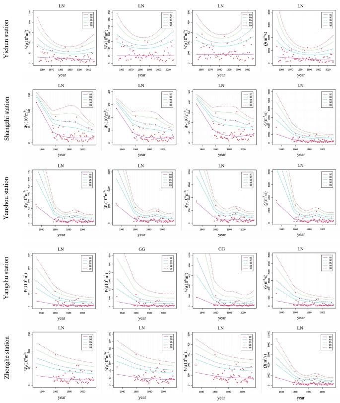
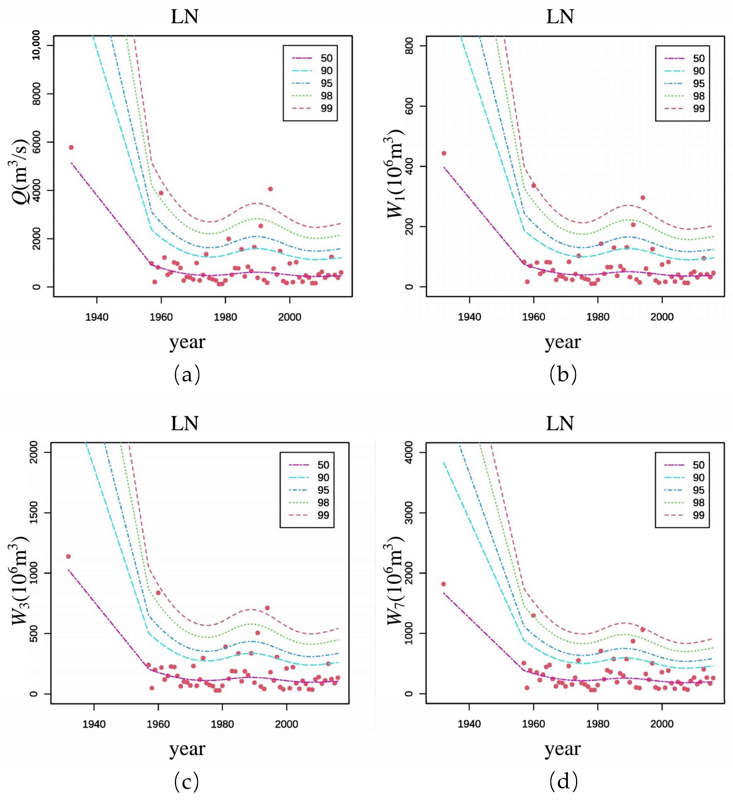
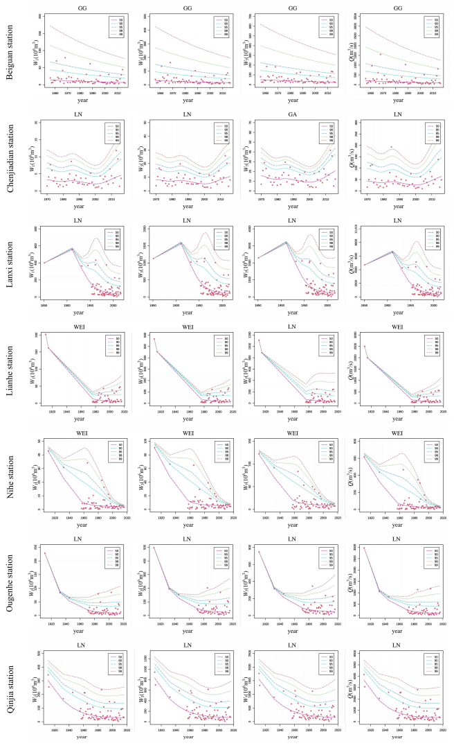
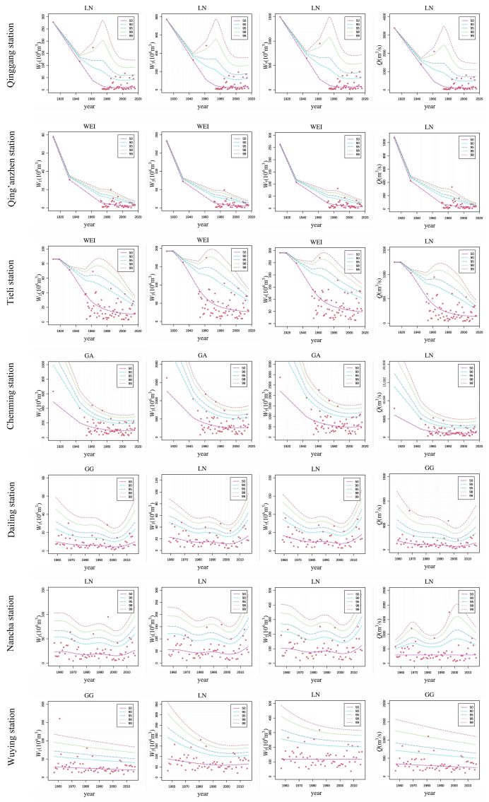
The optimal theoretical distribution of the Mayi River—Lianhua station, as determined by time-covariate GAMLSS, is used to calculate various centile curves. We are more interested in the centiles of the cumulative probability of the measured points (50%, 90%, 95%, 98%, and 99%, correlating to the exceedance probability of (1–50%), (1–90%), (1–95%), (1–98%), and (1–99%)) because the sequences that we study are flood sequences. Figure 3 displays the centile curves for the theoretical distribution of the flood extremum sequence of the fitted models (Appendix A.3 displays the centile curves plots for other stations). As shown in Figure 3, there is good agreement between the distribution of the measured scatters and the shape of the centile curves for the measured range of the data. However, the shape of the centile curve is greatly affected by the value of the historical flood sample (1932), and the maximum peak flow in 1932 is more than seven times the mean of the measured flow sequence and its centile curves have a significant turning point at the time of the first measured sample (1957). When the number of historical flood events is smaller, the results of time-covariate GAMLSS will cause the theoretical frequency of historical floods to differ significantly from the empirical frequency of samples. In addition, Lianhua Station experienced several moderate-strength floods between 1970 and 2000, and excessive floods occurred in 1991 and 1994, so the centile curves rose upward during this period. After 2000, with the relative decrease in flood event intensity, the several centile curves became stable again.
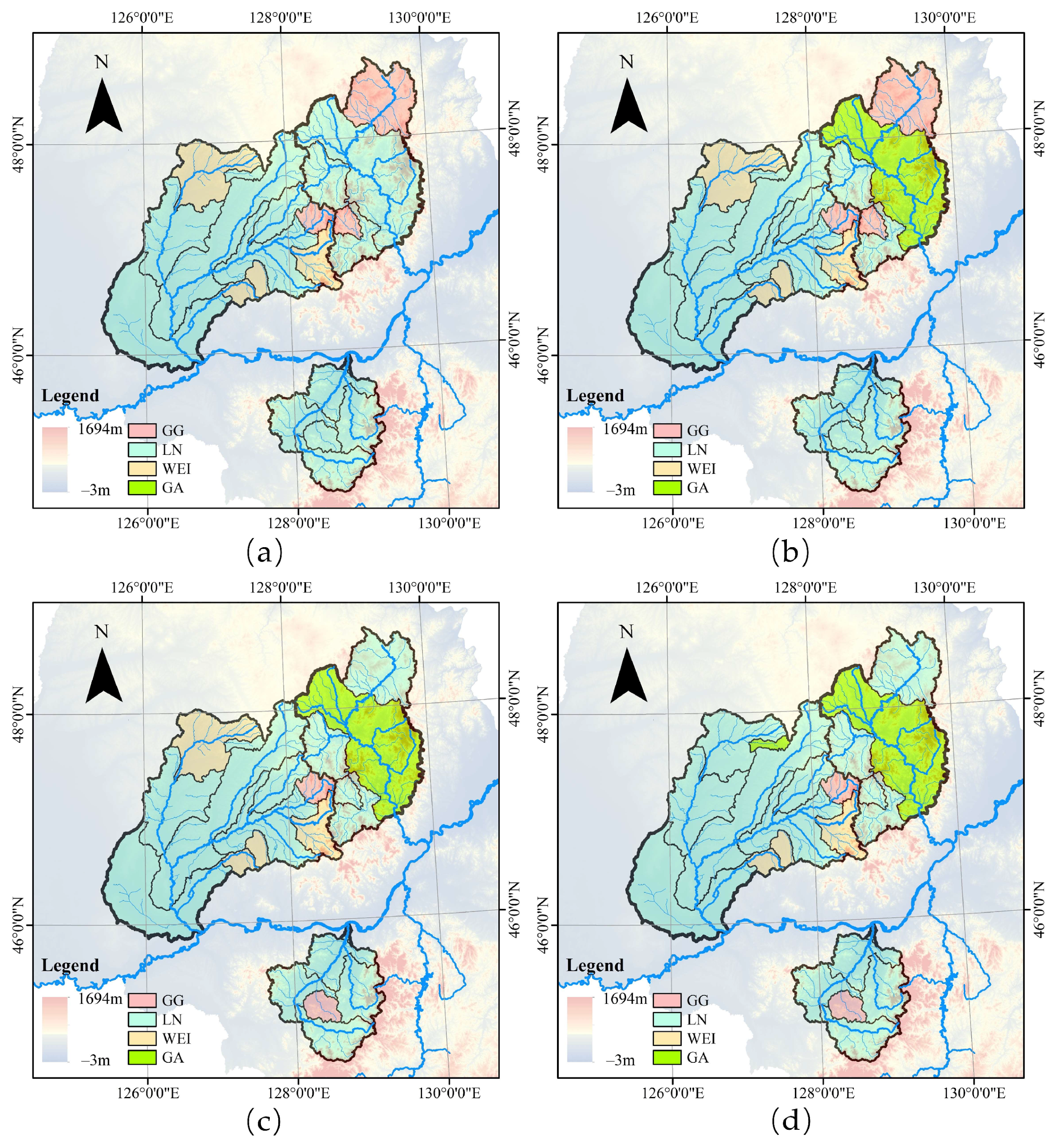
Across the study area, the accuracy of fitting the theoretical distribution of flood extremes varies considerably from station to station within different basins after the introduction of time covariates. Figure 4 presents the spatial distribution of the optimal theoretical distribution type of flood extremes derived from GAMLSS with time as a covariate. We discuss the distribution characteristics of the optimal distribution concerning terrain, basin area, etc. In the Hulan River basin, the station with the smallest AIC value is Chenjiadian Station, and its four flood characteristics’ AIC values are between 187.7 and 444.4. The station has a small basin area and a single terrain, which is hilly. The fitting accuracy is relatively high, including Lianhe Station (AIC value range: 310.5~525.5), Nihe Station (AIC value range: 228.0~610.8), Qing’anzhen Station (AIC value range: 227.3~472.1), etc. The AIC is the highest in the basin, i.e., the worst fitting station is Lanxi Station, and its AIC value is between 717.8 and 1052.7. Lanxi Station is the outlet station of the basin, and the terrain in the catchment area is complex, including plains, hills, and mountains. The above analysis shows that the complexity of the terrain in the basin area of the same basin will lead to obvious differences in the goodness of fit of the model. Similarly, the Tangwang River basin and Mayi River basin have the same characteristics. The AIC value range of Wuying Station upstream of the Tangwang River is 475.7~779.8. The terrain in the basin area of the station is a single mountain area, while the AIC range of Chenming Station in the outlet station is 751.0~1083.7. The optimal station for the Mayi basin is Yangshu Station, with an AIC value between 381.8 and 705.6. The station is located on the tributary of the Mayi River, with a small basin area and hilly terrain. The worst station in the Mayi River basin is Lianhua Station, and the AIC value range is 613.0~934.4. In summary, the station is located upstream of the basin with a small catchment area and a single terrain, and its fitting effect is significantly better than that of the downstream stations. The goodness of fit of the extreme value sequence model of the basin outlet hydrological station is the worst.

4.3. FFA by Precipitation-Covariate GAMLSS and Spatial Distribution of Optimal Theoretical Distribution

In this section, the steps of FFA considering precipitation covariates are roughly the same as those considering time covariates. The difference between the two sections is that the covariates of location and scale parameters are changed into precipitation variables P1 and P3 in the model. The model selection still uses the AIC criterion as the evaluation criterion to calculate the theoretical distribution of the flood sequence of each station. It is worth noting that when plotting the centile curve cluster of the optimal distribution in each station, the centile curves of the flood characteristics at all stations changed with the precipitation covariates, which showed a resemblance to the change in time covariates, which was greatly affected by the maximum cumulative precipitation. As there are different correspondences between different degrees of cumulative rainfall and flood characteristics, P1 corresponds better to Q and W1 than P3. However, when the dependent variables are W3 and W7, the precipitation parameter P1 is less able to explain these two flood characteristics than P3. The AMS method was also used to select the rainfall sequences in this paper, so the fields selected for P1 and P3 events are not necessarily the same for each year, and P3 is preferred for W3 and W7.
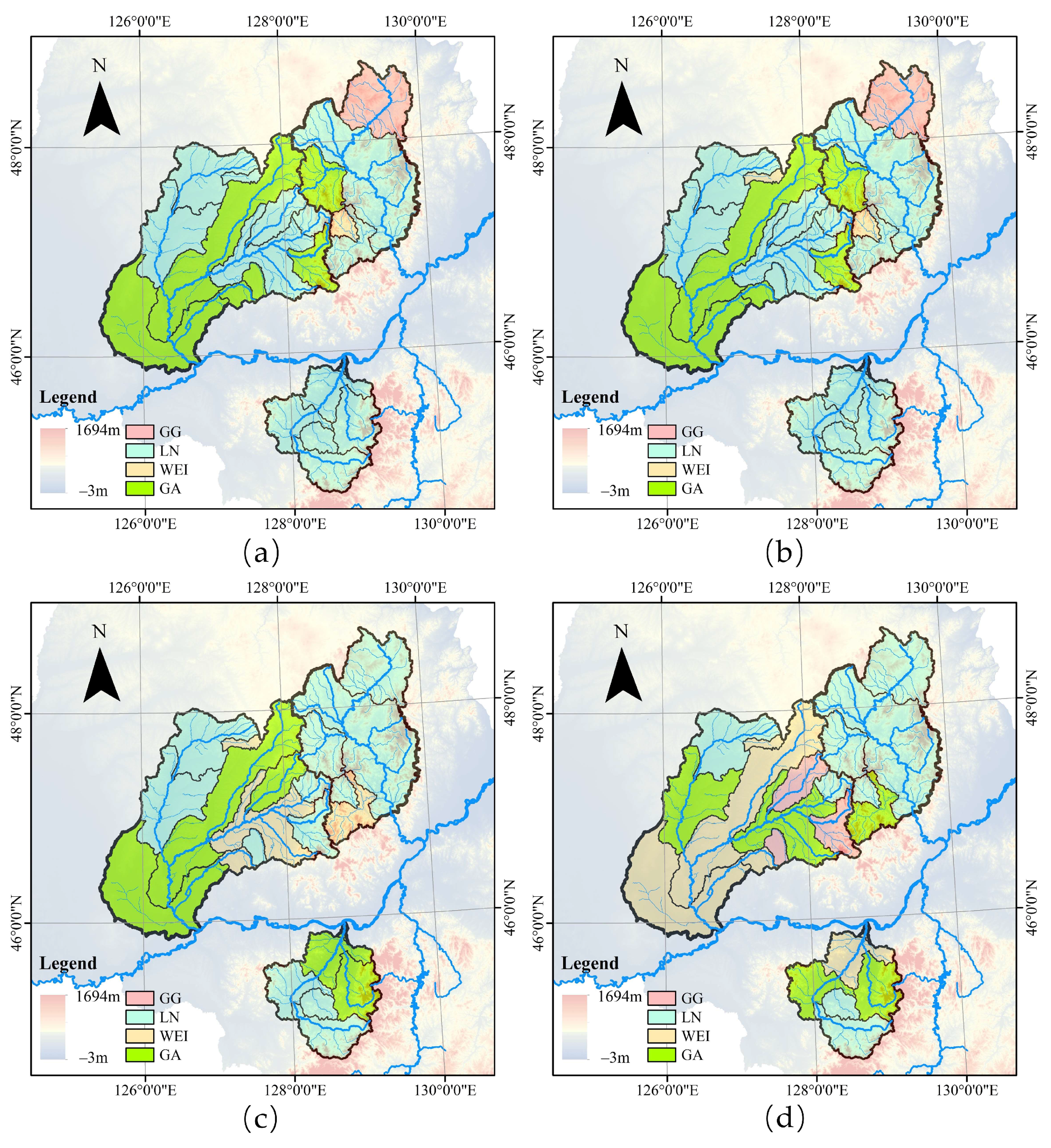
Figure 5 shows the centile curves of the four flood characteristics and precipitation-covariate GAMLSS at Lianhua Station. From this figure, it is shown that with the increase in the precipitation data value, the flood characteristic value has an overall upward trend. However, the shape of the centile curve is greatly affected by the values of the abnormal points, and Lianhua Station is still taken as an example. We find that the abnormal values occur in two models, Q and W1, and not in W3 and W7. It is seen that the covariate of the models Q and W1 is P1, and that of W3 and W7 is P3, and we analyze the generation of abnormal states from the covariate point. The black circle in Figure 5a,b demonstrates that the abnormal point value of the P1 sequence at Lianhua Station is larger (122.215 mm), but the corresponding flood feature sequence value is smaller (790 m3/s, 55.64 × 10⁶ m3), and the red circle in Figure 5a,b shows that the second-largest point of the P1 sequence value corresponds to a smaller flood characteristic as well. The year of occurrence of the P3 maximum point in the W3 and W7 models is the same (1966) as the year of occurrence of the P1 maximum point in the Q and W1 models. However, the red circles in Figure 5c,d show that the flood characteristics corresponding to the second-largest value point of the P3 sequence are much larger than those corresponding to the maximum value point, which is different from the models of Q and W1 in Figure 5a,b, where the maximum point in P1 leads to an abnormal downward trend in the second half of the centile curve of the precipitation-covariate GAMLSS and finally converges to this point. The abnormal point occurred in 1966, which is in the measured period of the sequences, and our data were extracted from the yearbook, which has high data reliability. Therefore, we did not process the data for the measured period before calculation, which led to the abnormal situation. This is also a reminder that variable–covariate correlations should be analyzed before model calculation and that outliers should be excluded in advance based on the historical situation to avoid the effect of abnormal data on the model calculation result. Based on the centile curve calculation results of all stations, it can be found that when the 90% quantile is selected, the deviation between the theoretical quantile frequency of the Tangwang River and the measured point frequency is the smallest, ranging from −5.0% to 3.4%. It is followed by the Mayi River basin, for which the deviation range is −7.4~2.5%. The largest deviation occurred in the Hulan River basin, which ranged from −9.6% to 5.7%. Compared with the time-covariate GAMLSS, the deviation range of the precipitation-covariate GAMLSS is slightly larger. The main reason may be the introduction of precipitation uncertainty information when the model is calculated with precipitation as a covariate. In the case of the time-covariate model, most of the data are measured. The occurred time, intensity, and flood characteristics of historical flood data have been verified by flood investigations, and the uncertainty is small. However, the situation for precipitation covariates is very different. The strength of the correspondence between precipitation data and floods, whether a single precipitation event can perfectly match each corresponding flood event, and the uncertainty of historical rainstorm data are greater. It is easy for abnormal points to affect the overall deviation. However, considering the above situation, the deviation of the simulation results is within a reasonable range. The spatial distribution of the optimal theoretical distribution of the GAMLSS preferences for different extreme flood characteristics at each station with precipitation as a covariate is shown in Figure 6.
The residual evaluation index of the GAMLSS with precipitation covariates shows that the mean value of the Mayi River’s residual sequence is −0.0404~0.0196, the variance is about 1.0021~1.0169, and the range of the Filliben coefficient is 0.9838~0.9957. In addition to the deviation of the W3 residual point distribution and y = x straight line (obviously jump phenomenon) in Hulan River—Lianhe Station and Tangwang River—Wuying station, the residual sequences of the flood characteristics of other stations can be considered as an approximate standard normal distribution, and the fit result of GAMLSS is good. Figure 6 shows that the optimal distribution of the mainstream of the Hulan River is different from the optimal distribution of its tributaries; except for W7, the optimal distribution of all flood characteristics is the gamma distribution. Looking at the terrain and precipitation-covariate GAMLSS optimal distribution types of the three basins together, we can find that the mountainous terrain optimal distribution types are mostly of a lognormal distribution, including most of the mountainous basins or the upstream mountainous parts of the plain basins.

4.4. FFA under Stationarity Assumption

To compare the FFA results in the nonstationary case with those under the assumption of stationarity, we assume that the probability distribution parameters of each flood extremum are constant. GAMLSS is used to solve the optimal theoretical distribution type of the flood extremum at each station. The calculation results and corresponding accuracy for the Mayi River basin are listed in Table 5 (the results for the Hulan River basin and Tangwang River basin are shown in Appendix A.4 and Appendix A.5), and the optimal fitting accuracy of the P-Ⅲ distribution is also given in Table 5.
The goodness of fit results between the empirical frequency data and optimal probability distribution curves of the Q, W1, W3, and W7 sequences fit by stationary GAMLSS are slightly worse than the flood characteristics fit by the P-Ⅲ distribution. It can be found from Table 5 that under the assumption of stationarity, from the results of AIC, the AIC values corresponding to the theoretical distribution of P-Ⅲ with an optimal value of 55.6% are smaller, and their fitting accuracy is similar to that of GAMLSS.

4.5. An Attempt to Apply NS-FFA in the Work of River Management Scope Demarcation

In recent years, many county regions have been strengthening the management and control of the shoreline spaces of rivers and lakes. According to the guidance issued by the Ministry of Water Resources in 2022, the first main point of this work is to “consolidate and improve the results of demarcation of the river and lake management scope and strengthen the spatial division and classification of coastlines in rivers and lakes”. At present, in the typical basins selected in this paper, the demarcation results of rivers with embankment sections can be determined according to the location of the embankment, while those rivers with embankment-free sections mostly use the intersection between the water line of a specific frequency of floods and the shoreline to determine the management scope. The specific frequency of 10% is the most commonly used design flood frequency. Moreover, the information shows that the frequency used in the delineation of river management scope in the typical basins in this paper is 10% (https://www.renrendoc.com/paper/286931603.html (accessed on 24 August 2023); http://www.hulan.gov.cn/art/2021/8/23/art_18976_1170318.html (accessed on 21 August 2023)). As a result, in this paper, a frequency of 10% was chosen for calculation. Based on the optimal theoretical distribution of each station, taking the corresponding flood extremum (Q, W1, W3, W7) calculation frequency p = 10% as an example, the calculation results and accuracy analysis are shown in Table 6. The values in the columns “stationarity assumption” and “nonstationarity assumption” of Table 6 are the simulated values of the model at corresponding frequencies, and the numbers in brackets are relative errors (used to express the calculation accuracy). Table 6 shows that, for a p = 10% flood, the calculated value of GAMLSS considering time covariates under the nonstationarity assumption is closer to the measured extremum sequence, absolute value of relative error is 0.12~15.78%, and the simulation accuracy is the highest among the four models. This indicates that using this model to consider the influence of time covariates is beneficial to improving the accuracy of the flood extremum frequency calculation results. In a frequency analysis, the model does not need to divide historical floods and measured floods but only needs to directly input the time corresponding to the flood extremum into the model. Compared with the traditional method with a P-III distribution, the hydrological frequency calculation process is simple and can be used as a basis for checking the rationality of design flood calculation results. The accuracy of GAMLSS under the stationarity assumption is equivalent to that of P-III, and the calculated values are larger than the measured values. The calculated results of this model are slightly better but inferior to those of GAMLSS with time covariates. It can be seen from the simulation results of GAMLSS with precipitation covariates that the influence of precipitation on the calculation results of this model is unstable. This might be because there is an error in adding some historical precipitation interpolation, or the precipitation events might not exactly match the flood events that correspond to the extreme value of the flood. However, the accuracy of the occurrence time of historical floods is relatively higher, which leads to the calculation accuracy of the precipitation-covariate model being relatively lower than that of GAMLSS with time covariates. In addition to the p = 10% frequency case, some flood characteristics at p = 20% frequency were simulated in these models. The conclusions drawn from the time-covariate model simulation results for all basins are consistent with those drawn in the case of a frequency of p = 10%, with the exception of the Hulan River basin, where the time-covariate model simulation performs poorly. This suggests that using time-covariate NS-FFA to demarcate the scope of river management in typical basins is more reliable. Even if there are unique frequencies, as in this work, NS-FFA can also be used by selecting other suitable models with a better simulation effect first.

5. Conclusions and Discussion

5.1. Conclusions

In order to determine the influence of historical flood events and precipitation extremum sequences on the result of FFA, this study used a comparative approach to find the most effective FFA method. Three basins with different terrain features in the Songhua River were taken as typical basins in this work. Firstly, the Mann–Kendall mutation test was used to diagnose the nonstationary nature of different flood extremum feature sequences. Then, based on the GAMLSS framework, the optimal theoretical distribution types of flood frequency under the nonstationarity assumption were studied by introducing time and precipitation covariates individually and determining the optimal distribution parameters. Finally, the FFA under the stationarity assumption was calculated, and the advantages and disadvantages of the model under the nonstationarity assumption were analyzed.
(1) There were mutation points in the sequences of flood extremum characteristics (Q, W1, W3, W7) in three typical basins of the Songhua River, and the mutation points were concentrated from 1960 to 1980 by the results of the Mann–Kendall mutation test and referring to the Pettitt test. The accuracy of the theoretical distribution in the nonstationary GAMLSS considering time and precipitation covariates is improved compared with both case models under the stationarity assumption. The optimal theoretical distribution considering time covariates fits all empirical frequencies better than the P-Ⅲ distribution, and fitting accuracy for optimal theoretical distribution considering precipitation-covariates is higher by 60% than the P-Ⅲ distribution. In the case of time-covariate models, the optimal distribution of the flood extremum in each typical basin is mainly LN (with 63.75%), followed by the WEI distribution (with 18.75%), and the optimal distributions of a few stations are the GG and GA distributions. In the case of precipitation covariates, the optimal distribution of the flood extremum in each typical basin is also mainly LN (with 57.5%). For all typical basins where covariates influence the theoretical distribution type of the flood extremum variables, the optimal theoretical distribution type considering time covariates can improve the accuracy of the flood frequency calculation results.
(2) The NS-FFA studies published so far usually focus on smaller basins and a few stations to calculate the nonstationary frequency. In this work, three typical basins and twenty hydrological stations were selected to analyze four flood characteristics and investigate the influence of terrain differences on the selection of the optimal distribution types. Among the three typical basins, the goodness of fit of GAMLSS in mountainous basins when calculating the flood extremum frequency was better than that in plain basins and mountain stream forest basins. It was found that the more unitary the basin terrain, the higher the goodness of fit of FFA by GAMLSS in nonstationary conditions, and vice versa. Hydrological stations in plain areas generally contain more terrain, and the goodness of fit of GAMLSS in the three typical basins was generally unsatisfactory. From the perspective of the spatial distribution of the GAMLSS optimal distribution, the distribution of time-covariate GAMLSS is strongly influenced by the hydrological stations’ data sequences, and the spatial distribution of sub-basins corresponding to different hydrological stations does not have strong regularity. For the precipitation-covariate GAMLSS, the mountainous area has a mostly lognormal distribution, while the plain area is dominated by a gamma distribution.
(3) The shape of the theoretical frequency curves is significantly influenced by the timing of historical floods and the connected precipitation events. If the correspondence is not good, it will generate abnormal points and cause the centile curve to be unusual. Therefore, the occurrence time of the flood extremum and corresponding precipitation should be carefully determined in the calculation of the flood frequency. The study illustrates that the time-covariate GAMLSS’ calculation result’s relative error is lower than the traditional model’s P-III distribution’s relative error. Thus, time-covariate GAMLSS has an advantage in NS-FFA. Moreover, it is unnecessary to deal with historical floods as in the uniform sample method; therefore, we can avoid the calculation of the historical flood frequency in traditional FFA, making the calculation process more convenient.
(4) The best nonstationary model’s fitting value for the time-covariate GAMLSS is slightly lower than the measured value in the demarcation work of the river management scope, according to the comparison of the stationary and nonstationary model calculation results and conclusion (1). The results of the calculation based on the time-covariate GAMLSS model lead to the design water surface line of the embankment-free sections being lower, which can reduce the area of the management scope and then reduce the pressure of the flood control management work, such as administrative approval for river projects. This work provides an alternative method of frequency analysis for demarcation.

5.2. Discussion

At present, many NS-FFA methods have been used in previous studies. The NS-FFA method, unlike S-FFA, has several sets of well-established standards that can be simply applied to almost any flood sequence. Instead, different results of different NS-FFA methods will appear for the same basin, showing a pluralistic condition. When considering different influenced covariates in NS-FFA, the optimal distribution type for flood sequences may change, which leads to changes in the final FFA results. Therefore, it is difficult to form a professional standard that can be simply applied to NS-FFA. Furthermore, the reasons that NS-FFA cannot be widely used also include the lack of hydrological data, short sequences, and the weak correspondence between covariates and flood events.
The traditional stationary FFA widely used in China is still the most reliable and universally operable FFA method. For water conservancy projects with high flood protection requirements, it often means a large investment, so it is important to improve the accuracy of FFA. In the example given in this paper, the relative error of the calculation results of the two cases under the stationarity assumption is positive, i.e., the calculated values are greater than the measured values, but the relative error value is large, which will lead to a waste of resources. The relative error of the results calculated by the time-covariate NS-FFA method is the smallest, but the value is smaller than the measured value. The results of these two cases are used as the design values, which obey the principle of unfavorable flood control that should be followed in the design of water conservancy projects. In the case of the simple precipitation-covariate NS-FFA method, the relative error of the gate station in basins is too large. Due to the poor correspondence between historical precipitation data, the calculation results are problematic. If only the measured precipitation sequence is selected for the NS-FFA of precipitation covariates, the accuracy of the calculation may be higher.
The data used in this work, excerpted from the hydrological yearbooks, had good reliability but less relative material. Therefore, the abnormal points of the precipitation–flood relationship were not addressed, which led to the unreasonable shape of the quantile curves in the precipitation-covariate GAMLSS. A data reliability analysis should be performed in further studies. Furthermore, we did not quantify the effect of terrain differences on the type of distribution, although the regularity was summarized. Thus, research from the perspective of quantifying the effect of terrain should be carried out in the future. In addition, NS-FFA under other specific frequencies (except p = 10%) should be applied to selected practical projects to test the applicability of the presented model.

Author Contributions

Conceptualization, M.L. and Z.X.; Methodology, M.L.; Software, M.L., H.L. and Y.X.; Validation, Y.W. and M.L.; Formal Analysis, J.S. and Q.H.; Investigation, M.L. and H.L.; Resources, Z.X.; Data Curation, H.L.; Writing—Original Draft Preparation, M.L.; Writing—Review and Editing, Z.X. and Y.W.; Visualization, M.L.; Supervision, Z.X. All authors have read and agreed to the published version of the manuscript.

Funding

This research was funded by the National Natural Science Foundation of China (grant number 51979038) and the Natural Science Foundation of Heilongjiang Province of China (grant number E2015024). The APC was funded by National Natural Science Foundation of China (grant number 51979038).

Data Availability Statement

The data presented in this study are available on request from the corresponding author. The data are not publicly available due to a privacy agreement. They were obtained from the Annual Hydrological Report P. R. China, Hydrological Data of Heilongjiang River Basin and Historical Floods in Heilongjiang Province.

Conflicts of Interest

The authors declare no conflict of interest.

Appendix A

Appendix A.1. Optimal Distribution of Flood Extreme Value Considering Time Covariates at Stations in Hulan River Basin

CharacteristicStationFitted DistributionLocation Parameter βScale Parameter σAICSBC
QBeiguanGG33.199 − 0.014 × t−0.383761.0769.5
ChenjiadianLN−1.199 + 0.002 × cs(t)−0.435444.4455.5
LanxiLN32.901 − 0.013 × cs(t,2)−88.292 + 0.044 × cs(t,2)1052.71070.5
LianheWEI49.277 − 0.022 × cs(t,1)168.934 − 0.085 × cs(t,1)525.5536.1
NiheWEI49.610 − 0.023 × cs(t,2)−7.317 + 0.004 × cs(t,2)610.8627.8
OugenheLN52.896 − 0.024 × cs(t,2)−93.045 + 0.047 × cs(t,2)613.2628.3
QinjiaLN43.224 − 0.019 × pb(t,2)−22.244 + 0.011 × pb(t,2)990.11004.9
QinggangLN30.922 − 0.013 × cs(t,2)−94.675 + 0.047 × cs(t,2)580.7595.4
Qing’anzhenWEI63.869 − 0.030 × cs(t,1)45.780 − 0.023 × cs(t,1)472.1483.2
TieliWEI25.759 − 0.010 × cs(t,2)58.709 − 0.029 × cs(t,2)876.7894.5
W1BeiguanGG29.009−0.014 × t−0.459428.4436.9
ChenjiadianLN−3.504 + 0.002 × cs(t)−0.587187.7198.8
LanxiLN30.416 − 0.013 × cs(t,2)−88.636 + 0.045 × cs(t,2)717.8735.6
LianheWEI47.539 − 0.023 × cs(t,1)164.278 − 0.082 × cs(t,1)310.5321.1
NiheWEI46.855 − 0.023 × cs(t,2)−7.646 + 0.004 × cs(t,2)288.0305.1
OugenheLN48.903 − 0.023 × cs(t,2)−93.097 + 0.047 × cs(t,2)366.1381.2
QinjiaLN41.257 − 0.019 × pb(t)−22.466 + 0.011 × pb(t)661.8676.5
QinggangLN28.487 − 0.013 × cs(t,2)−94.912 + 0.048 × cs(t,2)352.9367.6
Qing’anzhenWEI58.358 − 0.029 × cs(t,1)53.450 − 0.027 × cs(t,1)227.3238.4
TieliWEI20.827 − 0.009 × cs(t,2)59.334 − 0.030 × cs(t,2)519.8537.5
W3BeiguanGG −0.662518.3526.8
ChenjiadianLN1.570 + 0.0002 × cs(t)−0.643268.4279.5
LanxiLN30.966 − 0.013 × cs(t,2)−88.954 + 0.045 × cs(t,2)860.3878.1
LianheWEI49.792 − 0.023 × cs(t,1)161.483 − 0.081 × cs(t,1)398.8409.3
NiheWEI44.319 − 0.021 × cs(t,2)−7.795 + 0.004 × cs(t,2)394.0411.0
OugenheLN46.176 − 0.021 × cs(t,2)−94.088 + 0.047 × cs(t,2)455.9471.0
QinjiaLN42.423 − 0.019 × pb(t)−23.773 + 0.012 × pb(t)796.4811.0
QinggangLN29.497 − 0.013 × cs(t,2)−95.310 + 0.048 × cs(t,2)449.5464.1
Qing’anzhenWEI56.775 − 0.027 × cs(t,1)55.404 − 0.028 × cs(t,1)310.6321.7
TieliWEI20.538 − 0.008 × cs(t,2)58.328 − 0.029 × cs(t,2)636.7654.5
W7BeiguanGG14.859 − 0.0003 × bfp(t,2)−0.803572.8581.2
ChenjiadianGA−0.082 + 0.001 × cs(t)−0.666317.8328.9
LanxiLN31.515 − 0.013 × cs(t,2)−90.416 + 0.045 × cs(t,2)958.9976.6
LianheLN56.087 − 0.026 × cs(t,1)−124.62 + 0.062 × cs(t,1)458.0468.5
NiheWEI41.249 − 0.019 × cs(t,2)−4.250 + 0.002 × cs(t,2)449.9466.9
OugenheLN42.091 − 0.019 × cs(t,2)−94.626 + 0.047 × cs(t,2)510.7525.8
QinjiaLN43.256 − 0.019 × pb(t)−25.114 + 0.013 × pb(t)883.3897.7
QinggangLN30.062 − 0.013 × cs(t,2)−95.860 + 0.048 × cs(t,2)516.1530.8
Qing’anzhenWEI54.494 − 0.026 × cs(t,1)59.978 − 0.030 × cs(t,1)353.7364.8
TieliWEI19.522 − 0.008 × cs(t,2)58.085 − 0.029 × cs(t,2)702.7720.5

Appendix A.2. Optimal Distribution of Flood Extreme Value Considering Time Covariates at Stations in Tangwang River Basin

CharacteristicStationFitted DistributionLocation Parameter βScale Parameter σAICSBC
QChenmingLN27.311 − 0.010 × pb(t)−0.4451083.71092.9
DailingGG24.092 − 0.010 × cs(t)−0.565668.2682.6
NanchaLN5.661−12.681 + 0.006 × cs(t)818.6831.3
WuyingGG17.659 − 0.006 × t−0.783779.8788.2
YichunLN30.590 − 0.012 × pb(t)−2.680 + 0.001 × pb(t)847.7859.0
W1ChenmingGA26.682 − 0.011 × pb(t)−0.518751.0760.1
DailingGG14.653 − 0.006 × cs(t)−0.551341.1355.6
NanchaLN9.929 − 0.004 × cs(t)−0.455489.9502.6
WuyingGG14.925 − 0.006 × pb(t)−0.805475.7484.1
YichunLN21.341 − 0.009 × pb(t)−3.957 + 0.002 × pb(t)514.7525.7
W3ChenmingGA26.819 − 0.011 × pb(t)−0.539879.4888.5
DailingLN11.687 − 0.004 × cs(t)−0.543432.3444.7
NanchaLN8.864 − 0.003 × cs(t)−0.499592.7605.3
WuyingLN16.036 − 0.006 × pb(t)14.707 − 0.008 × pb(t)592.0602.7
YichunLN3.952−5.410 + 0.002 × cs(t,1)606.6615.0
W7ChenmingGA26.156 − 0.010 × pb(t)−0.565960.7969.8
DailingLN11.020 − 0.004 × cs(t)−0.576493.8506.1
NanchaLN9.494 − 0.003 × cs(t)−0.530661.4674.0
WuyingLN4.77811.547 − 0.006 × pb(t)662.9669.8
YichunLN4.479−7.616 + 0.004vcs(t,1)663.6672.1

Appendix A.3. Theoretical Optimal Time-Covariate Distribution Quantile Curves in Hulan, Tangwang, and Mayi River Basins
Water 15 03443 i001
Water 15 03443 i002
Water 15 03443 i003

Appendix A.4. Optimal Probability Distribution Results of Flood Extremum in Hulan River Basin under Stationary Condition

CharacteristicStationFitting Results ofP-Ⅲ DistributionFitting Results of Stationary GAMLSS
CvCsAICSBCFitted DistributionAICSBC
QBeiguan1.2932.627772.66766.33GG766.1772.4
Chenjiadian0.9471.969445.12450.67LN445.3449.0
Lanxi1.0412.1111097.711104.36LN1091.21095.6
Lianhe1.4112.842537.30542.58GG543.1548.4
Nihe1.5703.099621.46627.84LN623.0627.2
Ougenhe1.7343.476636.53642.20GG641.3647.0
Qinjia0.9811.9991012.501019.07LN1007.21011.6
Qinggang1.6233.253590.84596.33GG597.1602.6
Qing’anzhen1.6803.347489.65495.20GG490.5496.1
Tieli1.0062.081889.24895.90LN893.6898.0
W1Beiguan1.1002.119439.87433.54LN435.8440.1
Chenjiadian1.1621.682189.76195.31LN189.0192.7
Lanxi0.9982.006764.43771.09LN756.3760.8
Lianhe1.8533.533328.04333.33GG329.5334.8
Nihe1.4692.502298.42304.80LN302.6306.8
Ougenhe1.8343.512400.66406.34GG394.6400.3
Qinjia1.0002.005684.32690.89LN679.0683.4
Qinggang1.5683.054363.42368.90GG369.4374.8
Qing’anzhen2.0203.543252.19257.74GG246.7250.4
Tieli1.0462.051532.83539.49LN536.6541.1
W3Beiguan1.0172.071530.96524.63LN528.0532.2
Chenjiadian0.8631.655269.37274.92LN269.5273.2
Lanxi0.9952.013905.35912.01LN898.7903.1
Lianhe1.7433.448416.76422.04GG419.4424.7
Nihe1.3642.536401.64408.02LN410.3414.5
Ougenhe1.7043.363493.62499.29LN485.1488.9
Qinjia0.9521.925820.32826.89LN814.5818.8
Qinggang1.5022.988460.21465.70GG466.1471.6
Qing’anzhen1.6413.156327.82333.37LN328.5332.2
Tieli1.0322.107643.24649.90LN653.4657.8
W7Beiguan0.9462.003576.47582.80GG579.7586.0
Chenjiadian0.8911.799317.78323.33LN318.9322.6
Lanxi0.9932.0161003.491010.15LN997.91002.3
Lianhe1.5263.052471.83477.11GG478.6483.9
Nihe1.2512.383470.19476.57LN467.7472.0
Ougenhe1.5713.139541.53547.20LN539.0542.8
Qinjia0.9091.843907.10913.67LN902.2906.6
Qinggang1.9503.886530.84536.33GG533.8539.3
Qing’anzhen2.0773.971373.88379.43LN369.6373.3
Tieli0.9692.005717.55724.21LN720.9725.3

Appendix A.5. Optimal Probability Distribution Results of Flood Extremum in Tangwang River Basin under Stationary Condition

CharacteristicStationFitting Results ofP-Ⅲ DistributionFitting Results of Stationary GAMLSS
CvCsAICSBCFitted DistributionAICSBC
QChenming0.9682.0551085.471092.04LN1091.01095.4
Dailing1.3632.775683.76689.94LN672.6676.8
Nancha1.1002.310813.27819.60LN818.3822.5
Wuying1.8503.832827.67833.95GG780.7787.0
Yichun0.8231.717852.71859.04LN852.5856.8
W1Chenming0.9722.052752.32758.89LN758.8763.2
Dailing0.8901.649345.14351.32LN343.4347.5
Nancha0.8411.719488.68495.01LN488.8493.0
Wuying1.8493.592521.34527.63GG476.6482.9
Yichun0.8241.677515.70522.03LN516.2520.4
W3Chenming0.8321.775887.82894.39LN887.1891.4
Dailing0.8251.681434.87441.05LN435.9440.0
Nancha0.7911.680590.60596.93LN592.5596.7
Wuying1.8223.708646.57652.85GG593.6599.9
Yichun0.7581.596608.17614.51LN608.4612.6
W7Chenming0.8101.742968.66975.23LN967.8972.2
Dailing0.8521.794495.69501.87LN498.1502.2
Nancha0.5511.010663.39669.72GA659.8664.0
Wuying1.5903.317711.85718.13LN662.8667.0
Yichun1.2300.702677.03683.36LN665.2669.4

References

  1. Wei, Y.; Wang, X. (Eds.) Engineering Hydrology, 1st ed.; China Water & Power Press: Beijing, China, 2005; Chapter 4; pp. 59–73. ISBN 978-7-5084-2973-1. [Google Scholar]
  2. Intergovernmental Panel On Climate Change (Ipcc). Climate Change 2022—Impacts, Adaptation and Vulnerability: Working Group II Contribution to the Sixth Assessment Report of the Intergovernmental Panel on Climate Change, 1st ed.; Cambridge University Press: Cambridge, UK, 2023; ISBN 978-1-00-932584-4. [Google Scholar]
  3. Delgado, J.; Llorens, P.; Nord, G.; Calder, I.R.; Gallart, F. Modelling the Hydrological Response of a Mediterranean Medium-Sized Headwater Basin Subject to Land Cover Change: The Cardener River Basin (NE Spain). J. Hydrol. 2010, 383, 125–134. [Google Scholar] [CrossRef]
  4. Zhou, Y.; Zhang, S.; Wu, X.; Wang, D.; Li, H. The Research of long-term forecasting of non-stationary hydrologic time series based on the improved BP neural network. In Water Conservancy Information Technology Forum; Hohai University: Nanjing, China, 2020; pp. 92–99. [Google Scholar]
  5. Milly, P.C.D.; Betancourt, J.; Falkenmark, M.; Hirsch, R.M.; Kundzewicz, Z.W.; Lettenmaier, D.P.; Stouffer, R.J. Stationarity Is Dead: Whither Water Management? Science 2008, 319, 573–574. [Google Scholar] [CrossRef] [PubMed]
  6. Liang, Z.; Hu, Y.; Wang, J. Advances in hydrological frequency analysis of non-stationary time series. Adv. Water Sci. 2011, 22, 864–871. [Google Scholar] [CrossRef]
  7. Feng, P.; Zeng, H.; Li, X. Non-Stationary Flood-Frequency Analysis Based on Mixed Distribution. J. Tianjin Univ. (Sci. Technol.) 2013, 46, 298–303. [Google Scholar]
  8. Zhang, K.; Dong, X.; Liao, K.; Jiang, Z.; Cao, L. Characteristics of Seasonal Changes in Extreme Temperature and Their Relativity with ENSO in the Yellow River Basin from 1960 to 2017. Res. Soil Water Conserv. 2020, 27, 185–192. [Google Scholar] [CrossRef]
  9. Zhao, H.; Wang, Z.; Li, X.; Chu, Z.; Zhao, C.; Zhao, F. Research on the Evolution Characteristics of Future Climate Change in West Liao River Basin. Environ. Sci. Pollut. Res. 2022, 29, 509–517. [Google Scholar] [CrossRef]
  10. Jiang, C.; Xiong, L. Trend Analysis for the Annual Discharge Series of the Yangtze River at the Yichang Hydrological Station Based on GAMLSS. Acta Geophys. Sin. 2012, 67, 1505–1514. [Google Scholar]
  11. Zhang, Q.; Gu, X.; Singh, V.P.; Xiao, M.; Xu, C.-Y. Stationarity of Annual Flood Peaks during 1951–2010 in the Pearl River Basin, China. J. Hydrol. 2014, 519, 3263–3274. [Google Scholar] [CrossRef]
  12. Lu, F.; Xiao, W.; Yan, D.; Wang, H. Progresses on statistical modeling of non-stationary extreme sequences and its application in climate and hydrological change. J. Hydraul. Eng. 2017, 48, 379–389. [Google Scholar] [CrossRef]
  13. Dong, A. Study on Generalized Pareto distribution and its Application on Frequency Analysis of Hydrology. Master’s Dissertation, Hohai University, Nanjing, China, 2005. [Google Scholar]
  14. Wang, J.; Song, S. Application of generalized Pareto distribution in POT flood series frequency analysis. J. Northwest AF Univ. (Nat. Sci. Ed.) 2010, 38, 191–196. [Google Scholar] [CrossRef]
  15. Zhang, T.; Wang, Y.; Wang, B.; Tan, S.; Feng, P. Nonstationary Flood Frequency Analysis Using Univariate and Bivariate Time-Varying Models Based on GAMLSS. Water 2018, 10, 819. [Google Scholar] [CrossRef]
  16. Scala, P.; Cipolla, G.; Treppiedi, D.; Noto, L.V. The Use of GAMLSS Framework for a Non-Stationary Frequency Analysis of Annual Runoff Data over a Mediterranean Area. Water 2022, 14, 2848. [Google Scholar] [CrossRef]
  17. Shao, S.; Zhang, H.; Singh, V.P.; Ding, H.; Zhang, J.; Wu, Y. Nonstationary Analysis of Hydrological Drought Index in a Coupled Human-Water System: Application of the GAMLSS with Meteorological and Anthropogenic Covariates in the Wuding River Basin, China. J. Hydrol. 2022, 608, 127692. [Google Scholar] [CrossRef]
  18. Jiang, X.; Fan, J.; Zhang, J.; Tong, Z.; Liu, X. GIS-based Risk Assessment on Rain and Flood Disasters of Songhua River. J. Catastrophology 2009, 24, 51–56. [Google Scholar]
  19. Yin, X.; Li, G.; Wang, X. Reflections on flood management and disaster reduction in the Songhua River basin in the new period. China Flood Drought Manag. 2022, 32, 81–84. [Google Scholar] [CrossRef]
  20. Han, S.; Zhao, Y. Analysis of Variation Trend and Mutation Characteristics of Natural Runoff in the Upstream of the Hulanhe River Basin. Water Resour. Power 2020, 38, 46–50. [Google Scholar]
  21. Xu, H. Impact of Groundwater Irrigation on Ammonia Nitrogen Migration Process in Hulan River Basin. Master’s Dissertation, Jilin University, Changchun, China, 2020. [Google Scholar]
  22. Zhou, G. Study on the Intra-annual Runoff Distribution Characteristics in Hulan River Basin. Water Resour. Power 2018, 36, 39–43. [Google Scholar]
  23. Cui, W.; Gao, Q.; Bai, Y.; Chen, W. Two-level zoning of aquatic ecological function for management of small and medium-sized size rivers—Case study of Mayihe River basin in Harbin Region. J. China Inst. Water Resour. Hydropower Res. 2014, 12, 394–401. [Google Scholar] [CrossRef]
  24. Ren, Y. Analysis of the evolution of precipitation runoff in the Tangwang River Basin. Heilongjiang Hydraul. Sci. Technol. 2019, 47, 33–35+80. [Google Scholar] [CrossRef]
  25. Madsen, H.; Pearson, C.P.; Rosbjerg, D. Comparison of Annual Maximum Series and Partial Duration Series Methods for Modeling Extreme Hydrologic Events: 2. Regional Modeling. Water Resour. Res. 1997, 33, 759–769. [Google Scholar] [CrossRef]
  26. Pan, X.; Rahman, A. Comparison of Annual Maximum and Peaks-over-Threshold Methods with Automated Threshold Selection in Flood Frequency Analysis: A Case Study for Australia. Nat. Hazards 2022, 111, 1219–1244. [Google Scholar] [CrossRef]
  27. Liu, H. Study on the Inconsistency of Flood Extreme Value Sequence and Frequency Distribution Considering Covariates. Master’s Dissertation, Northeast Agricultural University, Harbin, China, 2021. [Google Scholar]
  28. Wei, F. Modern Statistical Diagnosis and Prediction Techniques of Climate, 2nd ed.; China Meteorological Press: Beijing, China, 2007; ISBN 978-7-5029-4299-1. [Google Scholar]
  29. Verstraeten, G.; Poesen, J.; Demarée, G.; Salles, C. Long-term (105 years) variability in rain erosivity as derived from 10-min rainfall depth data for Ukkel (Brussels, Belgium): Implications for assessing soil erosion rates. J. Geophys. Res. 2006, 111, D22109. [Google Scholar] [CrossRef]
  30. Stasinopoulos, M.D.; Rigby, R.A.; Heller, G.Z.; Voudouris, V.; Bastiani, F.D. Flexible Regression and Smoothing: Using GAMLSS in R, 1st ed.; Chapman and Hall/CRC: Boca Raton, FL, USA, 2017; ISBN 978-1-315-26987-0. [Google Scholar]
  31. Rigby, R.A.; Stasinopoulos, D.M. A Semi-Parametric Additive Model for Variance Heterogeneity. Stat. Comput. 1996, 6, 57–65. [Google Scholar] [CrossRef]
  32. Akaike, H. Akaike, H. A New Look at the Statistical Model Identification. In Selected Papers of Hirotugu Akaike; Parzen, E., Tanabe, K., Kitagawa, G., Eds.; Springer Series in Statistics; Springer New York: New York, NY, USA, 1974; pp. 215–222. ISBN 978-1-4612-7248-9. [Google Scholar]
  33. Schwarz, G. Estimating the Dimension of a Model. Ann. Stat. 1978, 6, 461–464. [Google Scholar] [CrossRef]
  34. van Buuren, S.; Fredriks, M. Worm Plot: A Simple Diagnostic Device for Modelling Growth Reference Curves. Stat. Med. 2001, 20, 1259–1277. [Google Scholar] [CrossRef]
  35. Filliben, J.J. The Probability Plot Correlation Coefficient Test for Normality. Technometrics 1975, 17, 111–117. [Google Scholar] [CrossRef]
  36. Bao, W.; Li, Y. Summary of dangerous reservoirs reinforcement in the 13th five-year plan in Heilongjiang province. Heilongjiang Hydraul. Sci. Technol. 2018, 46, 154–155+175. [Google Scholar] [CrossRef]
  37. Song, X. Non-stationary Statistical Model and Its Applications in Hydro-meteorological Frequency Analysis. Master’s Dissertation, China University of Mining and Technology, Beijing, China, 2017. [Google Scholar]
  38. de Medeiros, E.S.; de Lima, R.R.; de Olinda, R.A.; Dantas, L.G.; Santos, C.A.C. Dos Space–Time Kriging of Precipitation: Modeling the Large-Scale Variation with Model GAMLSS. Water 2019, 11, 2368. [Google Scholar] [CrossRef]
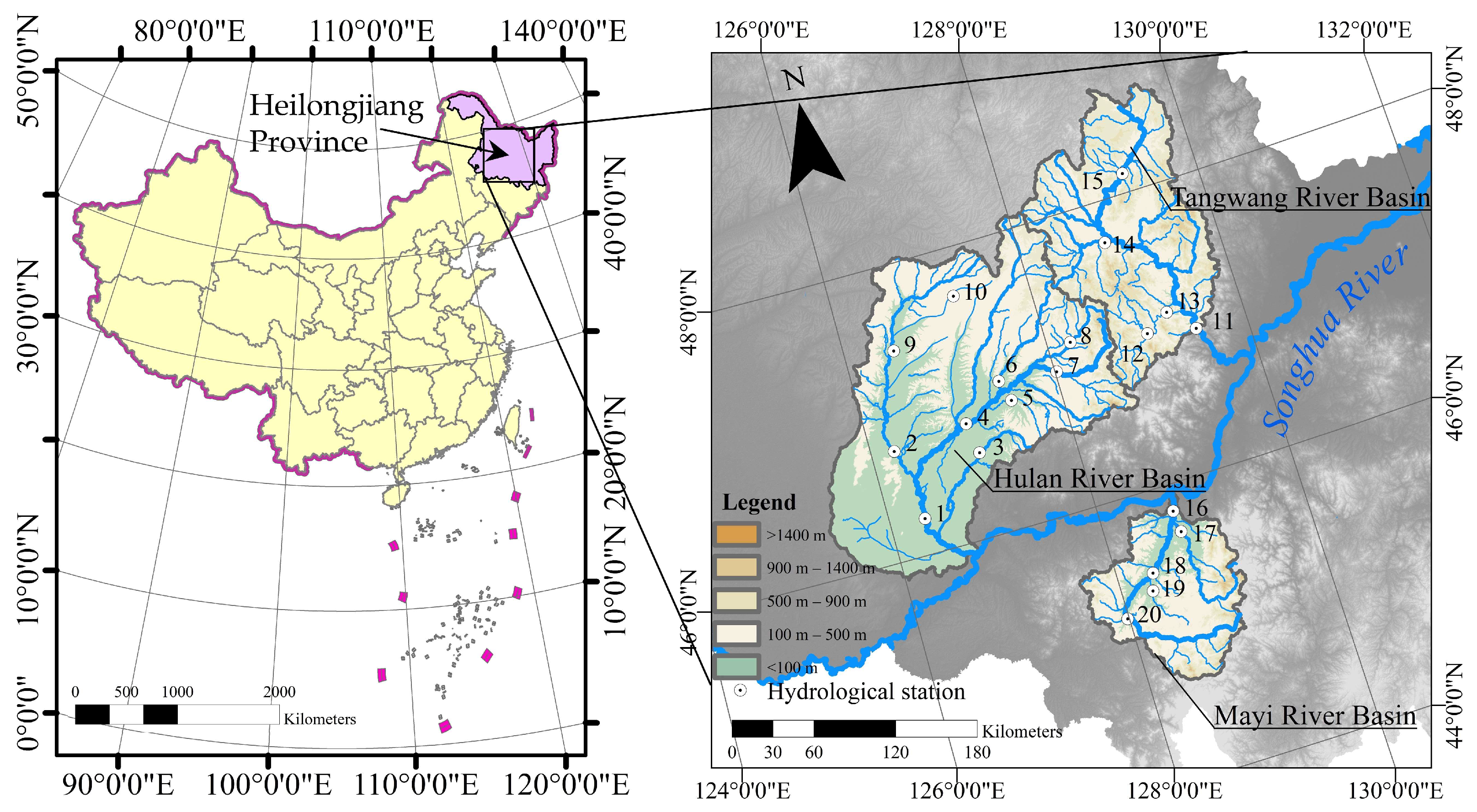
Figure 1. Locations and terrain of the river basins and hydrological stations. “·”: 1. Lanxi Station; 2. Qinggang Station; 3. Nihe Station; 4. Qinjia Station; 5. Qing’an Town Station; 6. Ougenhe Station; 7. Tieli Station; 8. Beiguan Station; 9. Lianhe Station; 10. Chenjiadian Station; 11. Chenming Station; 12. Dailing Station; 13. Nancha Station; 14. Yichun Station; 15. Wuying Station; 16. Lianhua Station; 17. Zhonghe Station; 18. Yanshou Station; 19. Yangshu Station; 20. Shangzhi Station.
Water 15 03443 g001
Figure 2. QQ-normal diagram and Filliben coefficients for optimal models of 4 flood characteristics in (ad) in Lianhua Station. (a) Q, (b) W1, (c) W3, (d) W7.
Water 15 03443 g002
Figure 3. Centile curves of the optimal model under time covariates for the 4 flood characteristics. (a) Q, (b) W1, (c) W3, (d) W7.
Water 15 03443 g003
Figure 4. Spatial distribution diagram of optimal theoretical distributions of different flood extremum considering time covariates. (a) Optimal models of Q, (b) optimal models of W1, (c) optimal models of W3, (d) optimal models of W7.
Water 15 03443 g004
Figure 5. Centile curves of the optimal models under precipitation covariate for the 4 flood characteristics. (a) Q, (b) W1, (c) W3, (d) W7.
Water 15 03443 g005
Figure 6. Spatial distribution diagram of optimal theoretical distributions of different flood extremum considering precipitation covariates. (a) Optimal models of Q, (b) optimal models of W1, (c) optimal models of W3, (d) optimal models of W7.
Water 15 03443 g006
Table 1. Flood sequences and the years of historical flood events of hydrological stations.
StationYears of
Dataset
Year(s) of Historical Flood Event(s)StationYears of
Dataset
Year(s) of Historical Flood Event(s)
Beiguan1956~2016/Chenming1954~20161911, 1945, 1951
Chenjiadian1970~2016/Dailing1959~2016/
Lanxi1953~20161851, 1911, 1932, 1945Nancha1956~2016/
Lianhe1976~20161911, 1915Wuying1957~2016/
Nihe1957~20161911, 1932Yichun1957~20161955
Ougenhe1971~20161911, 1932, 1945Lianhua1957~20161932
Qinjia1955~20161911, 1912, 1932, 1945Shangzhi1955~20161932
Qinggang1974~20161911, 1945, 1962Yanshou1958~20161932
Qing’anzhen1972~20161911, 1932Yangshu1957~20161932
Tieli1952~20161911, 1919, 1932Zhonghe1957~20161932
Table 2. Five selected distributions in GAMLSS.
NameProbability Density Functions (pdf)Parameter Link Functions
GA f y μ , σ = y 1 / σ 2 1 exp y / μ σ 2 μ σ 2 1 / σ 2 Γ 1 / σ 2
y > 0 , μ > 0 , σ > 0
E Y = μ ,   V a r Y = μ σ
g 1 μ = ln μ
g 2 σ = ln σ
LN f y μ , σ = 1 y σ 2 π exp log y μ 2 2 σ 2
y > 0 , < μ < , σ > 0
E Y = exp μ + σ 2 2
V a r Y = E 2 Y   ·   exp σ 2 1
g 1 μ = ln μ
g 2 σ = ln σ
WEI f y μ , σ = σ y σ 1 μ σ exp y μ σ
y > 0 , μ > 0 , σ > 0
E Y = μ Γ 1 σ + 1
V a r Y = μ 2 Γ 2 σ + 1 Γ 1 σ + 1 2
g 1 μ = ln μ
g 2 σ = ln σ
GG f y μ , σ , ν = ν θ θ z θ exp θ z y Γ θ , z = y μ ν , θ = 1 σ 2 ν 2
0 < y < , 0 < μ < , σ > 0 , < ν < , ν 0
E Y = μ , V a r Y = σ 2
g 1 μ = ln μ
g 2 σ = ln σ
g 3 ν = ν
GU f y μ , σ = 1 σ exp y μ σ exp y μ σ
y > 0 , < μ < , σ > 0
E Y = exp μ + σ 2 2 , V a r Y = E 2 Y   ·   exp σ 2 1
g 1 μ = μ
g 2 σ = ln σ
Table 3. Mutation years of hydrological stations by MK mutation test and Pettitt test.
Flood CharacteristicsHydrological Stations in Hulan River Basin
LanxiQinggangNiheQinjiaQing’an
Zhen
OugenheTieliBeiguanLianheChenjiadian
Q1967/19741981/19831998/19981969/19741998/19991988/19991969/19601981/19891982/19831973/2004
W11967/19671981/19831997/19981969/19741998/19991988/19991969/19741981/19901982/19831973/2004
W31967/19671979/19831998/19981969/19741998/19991988/19991966/19741981/19901982/19831973/2004
W71967/19741981/19831998/19981969/19741999/19991988/19991969/19741979/19901980/19831973/2008
Flood CharacteristicsHydrological Stations in Tangwang River BasinHydrological Stations in Mayi River Basin
ChenmingDailingNanchaYichunWuyingLianhuaZhongheYanshouYangshuShangzhi
Q1974/19751971/19741973/19741988/19911966/19751995/19981968/19981966/19981971/19921967/1975
W11974/19751968/19741974/19741990/19911972/19751995/19981969/19671966/19981971/19921967/1975
W31974/19751964/19751974/19741990/19921972/19751994/19981968/19671966/19981971/19921966/1975
W71974/19751964/19751974/19741991/19921966/19751995/19981967/19981966/19981971/19921960/1967
Table 4. Optimal distribution of flood extremes at each station in the Mayi River basin considering the time-covariate GAMLSS and the analytic expression of the parameters.
Flood CharacteristicStationOptimal DistributionLocation Parameter βScale Parameter σAICSBC
QLianhuaLN29.955 − 0.012 × cs(t)−0.298921.7934.4
ShangzhiLN34.507 − 0.015 × pb(t)−0.301835.5844.2
YanshouLN33.975 − 0.014 × cs(t)−0.277860.2872.8
YangshuLN38.396 − 0.017 × pb(t)−0.029697.9705.6
zhongheLN29.962 − 0.012 × cs(t)−0.283872.8885.5
W1LianhuaLN27.507 − 0.012 × cs(t)−0.328613.0625.7
ShangzhiLN33.475 − 0.015 × cs(t,2)−12.730 + 0.006 × cs(t,2)517.7534.9
YanshouLN31.388 − 0.014 × cs(t)−0.317552.3564.9
YangshuLN34.550 − 0.017 × pb(t)−0.061381.8389.6
zhongheLN16.055 − 0.007 × pb(t)−0.449474.4481.3
W3LianhuaLN28.917 − 0.012 × cs(t)−0.361733.0745.6
ShangzhiLN28.229 − 0.012 × pb(t)−0.392621.7630.8
YanshouLN31.122 − 0.013 × cs(t)−0.378660.2672.7
YangshuGG31.284 − 0.015 × cs(t,1)−0.216490.7501.3
zhongheLN16.899 − 0.007 × pb(t)−0.506581.6588.8
W7LianhuaLN29.649 − 0.012 × cs(t)−0.433802.0814.7
ShangzhiLN24.923 − 0.010 × cs(t,2)−9.153 + 0.004 × cs(t,2)677.7694.9
YanshouLN30.507 − 0.013 × cs(t)−0.453718.2730.7
YangshuGG32.119 − 0.015 × cs(t)−0.391541.4556.2
zhongheLN15.503 − 0.006 × pb(t)−0.598640.6647.9
Table 5. Optimal probability distribution results of flood extremum in Mayi River basin under stationarity assumption.
Flood CharacteristicStationFitting Results of P-Ⅲ DistributionFitting Results of Stationary GAMLSS
CvCsAICSBCBest Fit DistributionAICSBC
QLianhua1.1632.379926.96933.29GG927.5933.9
Shangzhi1.0712.201836.69843.12LN843.3847.6
Yanshou1.1112.276862.79869.07GG866.5872.8
Yangshu1.2522.519692.33698.66LN702.5706.7
Zhonghe0.9922.055874.12880.46LN875.7879.9
W1Lianhua1.2292.484610.81617.14GG619.4625.7
Shangzhi1.0012.001524.67531.10LN525.7530.0
Yanshou1.1162.246554.25560.53LN559.5563.7
Yangshu1.2202.223379.26385.60GG386.0392.3
Zhonghe0.8611.757475.73482.07LN474.7478.9
W3Lianhua1.2792.617721.90728.24GG740.3746.7
Shangzhi0.9912.045627.19633.62LN629.5633.8
Yanshou1.0882.238660.12666.40LN667.3671.5
Yangshu1.1772.300483.25489.58GG494.4500.8
Zhonghe0.8261.766582.06588.39LN582.2586.4
W7Lianhua1.1952.481790.90797.23LN809.9814.1
Shangzhi0.8881.883683.23689.66LN684.7689.0
Yanshou0.9762.045723.05729.34LN725.5729.7
Yangshu1.0582.121544.10550.43GG545.6552.0
Zhonghe0.8361.847638.67645.00LN640.9645.1
Table 6. Comparison of Q, W1, W3, and W7 flood extremum and simulated values in typical Songhua River basin. The measured extremum sequence consists of the measured point of flood frequency closest to the frequency quantile (10%), and the empirical frequency value corresponding to the measured extremum is in brackets. * indicates the case where the optimal distribution corresponds to the lowest relative error in four cases.
Flood
Characteristic
Typical Basinp = 10% Flood’s Extreme ValueMeasured Sequence Extremum
Stationarity AssumptionNonstationarity Assumption
P-ⅢGAMLSS-StationaryGAMLSS-TimeGAMLSS-Precipitation
Q
(m3/s)
Hulan2668.21 (+32.75%)2376.811 (+18.25%)1882.199 (−6.36%) *2641.498 (+31.42%)2010 (11.4%)
Tangwang3694.11 (+27.38%)3143.928 (+8.41%) *2595.534 (−10.50%)4211.814 (+45.23%)2900 (10.4%)
Mayi2038.91 (+23.57%)1715.71 (+3.98%)1644.117 (−0.36%) *3165.404 (+91.84%)1650 (9.28%)
W1
(106 m3)
Hulan222.98 (+31.00%)202.676 (+19.08%)160.3656 (−5.78%) *209.260 (+22.94%)170.208 (11.4%)
Tangwang301.4 (+37.88%)254.205 (+16.29%)195.572 (−10.53%) *332.363 (+52.05%)218.592 (10.4%)
Mayi178.74 (+36.10%)136.591 (+4.01%)131.482 (+0.12%) *247.202 (+88.23%)131.328 (9.28%)
W3
(106 m3)
Hulan630.26 (+27.08%)576.242 (+16.19%)453.966 (−8.46%) *445.035 (−10.26%)495.936 (11.4%)
Tangwang749.19 (+19.60%)673.833 (+7.57%)*527.561 (−15.78%)679.182 (+8.43%)626.4 (10.4%)
Mayi486.91 (+44.50%)365.005 (+8.32%)348.004 (+3.28%) *369.042 (+9.52%)336.96 (9.28%)
W7
(106 m3)
Hulan1299.3 (+24.28%)1191.927 (+14.01%)936.618 (−10.41%)950.234 (−9.11%) *1045.44 (11.4%)
Tangwang1389.76 (+26.65%)1249.309 (+13.85%)991.495 (−9.65%) *1258.202 (+14.66%)1097.366 (10.4%)
Mayi845.45 (+46.71%)643.986 (+11.75%)597.305 (+3.65%) *637.124 (+10.56%)576.288 (9.28%)
Disclaimer/Publisher’s Note: The statements, opinions and data contained in all publications are solely those of the individual author(s) and contributor(s) and not of MDPI and/or the editor(s). MDPI and/or the editor(s) disclaim responsibility for any injury to people or property resulting from any ideas, methods, instructions or products referred to in the content.