A Machine Learning-Based Framework for Water Quality Index Estimation in the Southern Bug River

Abstract

River water quality is of utmost importance because the river is not only one of the key water resources but also a natural habitat serving its surrounding environment. In a bid to address whether it has a qualified quality, various analytics are required to be considered, but it is challenging to measure all of them frequently along a river reach. Therefore, estimating water quality index (WQI) incorporating several weighted analytics is a useful approach to assess water quality in rivers. This study explored applications of ten machine learning (ML) models to estimate WQI for the Southern Bug River, which is the second-longest river in Ukraine. The ML methods considered in this study include artificial neural networks (ANNs), Support Vector Regressor (SVR), Extreme Learning Machine, Decision Tree Regressor, random forest, AdaBoost (AB), Gradient Boosting Regressor, XGBoost Regressor (XGBR), Gaussian process (GP), and K-nearest neighbors (KNN). Each data measurement consists of nine analytics (NH₄, BOD₅, suspended solids, DO, NO₃, NO₂, SO₄, PO₄, Cl), while the quantity of data is more than 2700 data points. The results indicated that all ML models demonstrate satisfactory performance in predicting WQI. However, GP outperformed the other models, followed by XGBR, SVR, and KNN. Furthermore, ANN and AB demonstrated relatively weaker performance. Moreover, a reliability assessment conducted on both training and testing datasets also confirmed the results of the comparative analysis. Overall, the results enhance the assertion that ML models can sufficiently predict WQI, thereby enhancing water quality management.

1. Introduction

Water is one of the most valuable resources, and its quality as well as its quantity, plays a crucial role for the survival of living beings on the earth [1,2]. Subpar water quality not only jeopardizes the wellbeing of humans and animals but also affects crop yields, resulting in economic losses [3]. Consequently, it is essential to conduct quality assessments of water from various sources to address this pressing issue [4].

Numerous water quality parameters exist, making it impossible to simultaneously consider all of them. Consequently, these parameters are condensed into a single index. Among the various available water quality indexes, one notable example is the Water Quality Index (WQI) [5]. Multiple approaches, including statistical and machine learning (ML) methods, have been employed to assess WQI.

Assessment of water quality based on ML models has gained prevalence. For instance, Haghiabi et al. [6] employed an artificial neural network (ANN), support vector machine (SVM), and group method of data handling (GMDH) for water quality prediction. They reported that all three ML techniques have the capability to predict water quality, while the performance of GMDH is lower than those of SVM and ANN. Furthermore, Bui et al. [7] compared performances of various ML algorithms in standalone and hybrid states and found that hybrid models performed better than the other ones. El Bilali and Taleb [8] utilized different ML techniques to evaluate water quality for irrigation and suggested the implementation of automated sensors coupled with ML models for real-time monitoring of water quality. Aldhyani et al. [9] developed multiple ML models to predict WQI, of which SVM achieved the highest accuracy. In addition, Tiyasha et al. [10] presented a detailed survey on applications of artificial intelligence techniques for surface water quality assessment. Since water quality is subjected to temporal variation and several factors affect water quality, they recommended that there is a need not only to monitor water quality continuously but also to evolve ML models to understand the nonlinearity in water quality in a better way. Kouadri et al. [11] employed eight ML algorithms to forecast WQI in southeast Algeria. They tested two scenarios for WQI computations, finding that multiple linear regression (MLR) had higher accuracy in the first scenario, while random forest performed better in the second scenario. Additionally, Asadollah et al. [12] exploited the extra tree regression (ETR) model to predict monthly WQI values in the Lam Tsuen River, Hong Kong, comparing it with SVM and decision tree regression (DTR), and ETR demonstrated superior performance. Ahmed et al. [13] applied a multilayer perceptron neural network (MLP), long short-term memory (LSTM), and a convolutional neural network to predict water quality and found that LSTM performed better than other two models. Uddin et al. [14] compared SVM, Naïve Bayes, Random Forest, KNN and gradient boost algorithms for water quality classification and found that the gradient boosting technique is the most suitable for classification. Recently, Goodarzi et al. [15] applied gene expression programming, model tree (M5P), and multivariate adaptive regression splines (MARS) for exploring the water quality of wells in Iran and found that MARS slightly improved on the estimates resulting from the other two models. The literature review includes an appraisal of ML models to estimate water quality assessment, as an alternative to applying statistical methods. In this paradigm, with the emergence of new advanced ML models, more studies are required to examine applicability of available ML models for water quality predictions. In other words, the use of advanced ML models in assessing water quality indices is essential because it allows more accurate estimations of WQI. Traditional models, like decision tree regressors (DTRs), obviously have limitations in capturing complex relationships, leading to less precise WQI predictions. With the advancement of ML methods, models like XGBoost, which is an advancement on DTR, have proven to be more capable of handling intricate patterns and improving overall performance in many problems. Thus, this study evaluated advanced ML models, like XGBoost, in comparison with traditional ML models for water quality assessment. Therefore, the choice of advanced ML models in our study was motivated by the potential to enhance accuracy and reliability in water quality forecasts.

In the present study, the capability of ten ML approaches to predict water quality was explored and their reliability compared through a reliability analysis. The ML models employed in this study include artificial neural networks (ANNs), Support Vector Regressor (SVR), Extreme Learning Machine (ELM), DTR, random forest regression (RFR), AdaBoost (AB), Gradient Boosting Regressor (GBR), XGBoost Regressor (XGBR), Gaussian process (GP), and K-nearest neighbors (KNN). According to the literature, a few of the applied techniques in the present study are novel in the field of water quality assessment. Additionally, a ranking scheme based on six metrics was used to evaluate and ranked all ML methods.

2. Materials and Methods

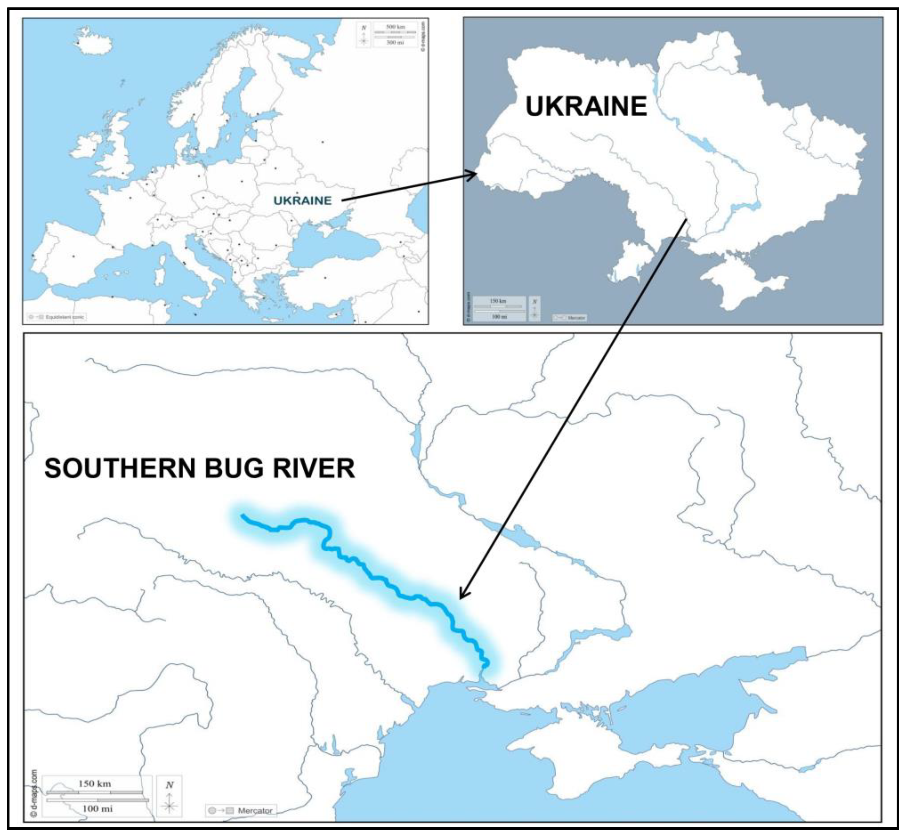
2.1. Study Area and Data Collection

The Southern Bug River (Figure 1) in Ukraine was considered for the present study. The river originates from the marshy regions near the town of Elnya in the Smolensk Region, courses towards Kiev, and eventually joins the Dnieper River. With a 792 km length and a drainage basin spanning 63,700 km², the Southern Bug River is the second-longest river in Ukraine [16]. It has a depth ranging from 1.5 to 8.0 m, and its total volume of average perennial runoff is 2.9 km³. Most of the annual runoff of the Southern Bug River (56%) originates from the forest-steppe region of its basin, while only 17.5% of the total annual river flow comes from the steppe region, primarily in the lower part of the basin. The regions near the middle lower part of the Southern Bug River experience moderately continental climatic conditions typical of the steppe zone characterized by insufficient humidification and hot summers with frequent arid spells, as well as warm and dry winters with snow, wet snow, and rain precipitation.

The water quality data were obtained from UCI (University of California Irvine) repository, covering a period of 21 years (2000–2021), consisting of 2776 instances [17]. The data were acquired from 22 monitoring stations located on the Sothern Bug River. The measured parameters are NH₄, BOD5, suspended solids, DO, NO₃, NO₂, SO₄, PO₄, and Cl. A statistical description of the data is presented in

Table 1. Descriptive statistics of parameters involved with the WQI computation for the Southern Bug River.

Parameters	Unit	Mean	Minimum	Maximum	Standard Deviation	Variance	Range
BOD5	mg/L	4.31	0	50.90	2.97	8.84	39.42
Suspended solids	mg/L	12.93	0	595.00	16.54	273.67	595.00
DO	mg/L	9.50	0	90.00	4.42	19.60	90.00
NO3	mg/L	4.31	0	133.40	6.88	47.35	133.40
NO2	mg/L	0.24	0	109.00	2.18	4.76	109.00
SO4	mg/L	59.36	0	3573.40	96.58	9328.20	3573.40
PO4	mg/L	0.41	0	13.879	0.77	0.59	13.87
Cl	mg/L	93.73	0.02	5615.28	394.51	155,639.90	5615.26
NH4	mg/L	0.75	0	39.42	2.48	6.18	39.42

. The statistical description provided in Table 1 can be used to gain insight into the distribution, variability, and range of values for each parameter in the dataset.

The dataset was split into two portions, with 80% of the complete data used for training (2221 data samples) and the remaining 20% set aside for testing ML models (555 data samples). This approach ensures that the models are trained on a large enough dataset to capture the underlying patterns and relationships within the data, while also having enough data reserved for testing to evaluate performances of the ML models.

2.2. Water Quality Index

Surface WQI is a technique which has been widely employed to categorize and convey a thorough assessment of the state of water quality in rivers. This method involves transforming the data obtained from extensive and intricate water quality monitoring programs into singular numerical values. In this study, the calculation of the WQI incorporates 9 parameters. These parameters include BOD₅, suspended solids, NH₄ dissolved oxygen, NO₃, NO₂, SO₄, PO₄, and Cl (as listed in Table 1).

The computation of WQI for a water sample involved three distinct stages:

(1)

To evaluate the overall quality of water, experts assigned weights (A_wj) ranging from 1 to 4 to each chemical parameter. These weights, based on previous studies [18,19,20], were utilized to assess the impact of each parameter on the overall water quality assessment. The calculation of the relative weight (R_w) for this study was performed using the following Equation (1).

$$R_w=\frac{A_{wj}}{{\sum }_{j=1}^n{A}_{wj}}$$

(1)

where A_wj refers to the assigned weight, R_w is a relative weight, and n signifies the parameter count.

(2)

A quality rating scale (Q_j) for each parameter is determined by dividing its annual mean concentration by its standard value [21].

$$Q_j=\frac{m_j}{s_j}\times 100$$

(2)

where $Q_j$ refers to the quality rating scale, $m_j$ denotes the observed value of the parameters, and $s_j$ is the standard parametric value.

(3)

To obtain the sub-indices (Si_j), the assigned weight is multiplied by the relative weight. WQI is then calculated by summing up these sub-indices using Equation (4):

$${Si}_j=R_w\times Q_j$$

(3)

$$WQI={\sum }_{j=1}^n{Si}_j$$

(4)

2.3. Machine Learning Models

2.3.1. Artificial Neural Networks

ANN is a well-known ML technique that was not only inspired by the learning behavior of human minds but also mimics it. In essence, data flows through a layer-based structure consisting of neurons to minimize a fitness function, which basically is an error between estimated values and benchmark solutions. To be more specific, the first layer entails input data, which in this study are the normalized water quality parameters. Furthermore, the last layer accommodates output data, which is WQI in the current study. Between the input and output layers, one or more than one layer, which is called a hidden layer, can be considered. In this study, the network comprises of two hidden layers, and each one has five hidden neurons in the ANN configuration. Moreover, each individual layer consists of a certain number of neurons. The neurons positioned within a specific layer are connected to the neurons in adjacent layers, while no connection among neurons of a single layer is allowed. This architecture enables ANN to serve as a suitable ML model in various fields of research, particularly for water quality [22,23,24,25] and other applications in water resources management [26,27].

2.3.2. Extreme Learning Machine

An ELM is an advanced ML tool with a single hidden-layer feedforward neural network in its configuration [28]. It incorporates the least-square method not only for calculating the weights between the hidden and output layers of the network but also for generating the parameters of hidden nodes randomly. The output layer of the network is trained using the Moore–Penrose generalized inverse, which allows fast and efficient training in comparison to the classical neural networks (Figure 2). At its core, ELM involves the process of solving a set of linear equations to determine the output weights, which minimize the difference between network predictions and the actual target. Because of its superior performance, fast learning, and better generalization ability, ELM has become a go-to technique for solving classification, regression, and patternrecognition-based problems.

Despite the ELM’s generally desirable performance, there are some shortcomings that can reduce its prediction accuracy. For example, in the training phase, non-optimal or unnecessary weight values and thresholds negatively impact the performance of the ELM and subsequently lead to unstable results. In addition, the ELM requires many hidden-layer nodes in its configuration, which often may yield overfitting and other issues.

2.3.3. Decision Tree Regressor

DTR is one of the excellent examples of supervised ML models that can be utilized for both regression and classification problems. Generally, each decision tree comprises of a root node at the top of the tree, internal nodes (i.e., branches), and leaf nodes at the bottom of the tree. At each node of the tree, the decision-making process involves employing conditional “if-else” statements, while progression through the tree is from the root node towards the leaf nodes [29]. Basically, decision trees split the training dataset into sub-categories based on conditional “if-else” statements. Each new data point is typically classified into a specific leaf node according to the predefined thresholds established using independent variables. The final output of the model is determined by calculating an average of the target variable values associated with all instances falling within a specific leaf node.

2.3.4. Random Forest

RF is a supervised ML algorithm widely applied for both regression and classification problems. This ensemble learning method constructs multiple decision trees (Figure 3), each one trained on a randomly selected subset of the data and features use of bagging or bootstrap aggregation [30]. The decision trees are combined to produce the final output, which is determined by aggregating the predictions of all individual trees [26]. Furthermore, the final output of RF is the mode of classes for classification and the mean prediction for regression, respectively. This method reduces overfitting and provides accurate and robust results for many ML applications, particularly in the field of water resources management.

2.3.5. Boosting-based Algorithms

Boosting algorithms are supervised ML models that ensemble multiple weak learners, such as decision trees, to enhance their overall accuracy and predictive ability. They commence with constructing one weak learner, while subsequent trees are iteratively produced based on minimizing the error made in the very previous iteration. Essentially, each weak learner has a weight based on its relative predictive ability, while adding new weak learners modifies the weights. The process of assembling weak learners continues until the error is minimized or a predefined threshold is met [27]. This study utilized three boosting-based algorithms including AdaBoost (AB), Gradient Boosting Regressor (GBR), and XGBoost Regressor (XGBR). More detailed information regarding these boosting-based algorithms can be found in [26].

2.3.6. Gaussian Process

GP is a kernel-based model that exploits a Gaussian distribution process before the regression analysis of data. GP is effective for both linear and non-linear problems because it does not assume a fixed number of parameters [31]. The two main functions in GP are (i) the covariance function that quantifies the resemblance between the input vectors of the training and testing datasets, and (ii) the mean function that governs the complexity of the model. It is noteworthy that the former often holds a greater significance than the latter [27]. Finally, GP utilizes the covariance function to predict new data points by computing the joint distribution involving both training and testing data.

2.3.7. K-Nearest Neighbors

KNN is a simple algorithm that can be used to predict a new data point based on its nearest neighbors, which are the closest training data points. In essence, KNN locates the K nearest data instances to a specific testing data point and computes a weighted average of their corresponding target values. To find the nearest neighbors, the algorithm must assess the resemblance between data points in the training dataset and the given testing data point. For this purpose, it employs a distance function. For continuous variables, the most frequently implemented distance functions include Euclidean, Manhattan, and Minkowski [27]. One of the most common distance functions is the Euclidean distance, which can be calculated using the following equation:

$$D=\sqrt{{\sum }_{i=1}^n{w}_i{\left[x_i\left(train data point\right)-x_i\left(test data point\right)\right]}^2}$$

(5)

where D represents the distance function, w is the weight of the ith feature, and x = (x₁, x₂, …, x_n) is the vector of the input features.

2.3.8. Support Vector Machine

An SVM is a highly adaptable and potent supervised ML algorithm that addresses complex classification, regression, and outlier detection problems by executing optimal data transformations. These transformations create boundaries using an optimal hyperplane between the data points, based on pre-defined classes, labels, or output [27]. The hyperplane is positioned in such a way that it maximizes the margin between the classes being considered.

As illustrated in Figure 4, the margin signifies the widest gap that runs parallel to the hyperplane, without including any internal support vectors. This gap is easy to define for linearly separable issues, but real-life scenarios can be more complex. Therefore, the SVM algorithm endeavors to maximize the margin between the support vectors, which can lead to incorrect classifications of smaller sections of data points.

The simulated outcome of an SVM model can be generated using Equation (6):

$$O =\beta +\Sigma {\mathbb{C}}_{i}K\left(x_i,x\right)$$

(6)

where $O$ is the predicted value, $\beta$ is the bias term, ${\mathbb{C}}_i$ is the coefficient of each input data point in the model, x_i is the input data point, $K$(x_i, x) is the kernel function used to compute the similarity between the input data point x_i and the new data point x.

2.4. Model Development

This study compared ten ML models (SVR, ELM, ANN, DTR, RF, AB, GBR, XGBR, GP, KNN) to forecast WQI for the Southern Bug River, Ukraine. The data used for the model development was divided into training and testing parts. Following the data division, the predictors and their corresponding WQI values were normalized between zero and one to enhance the learning processes of the ML models. IN addition, a grid search method was used to tune the hyperparameters of each ML model. The outputs of the ML models were then compared with the desired outputs, and the difference was referred to as error. The ML techniques were developed and run in the MATLAB and Python environments. The analysis of the ML methods was based on an iterative process, which required the selection of optimal hyperparameters through a grid search. Hence, to enhance the accuracy of the ML models, the optimal parameter values were determined, and modelling was performed accordingly. The entire process of training the ML models is illustrated in Figure 5, while the hyperparameters for each ML model are provided in

Table 2. Hyperparameters used for the applied ML models.

Model	Hyperparameter
SVR	Box constraint = 1
	Epsilon = 7.268
	Kernel scale = 1
	Solver = ISDA
	Iteration = 1000
KNN	Algorithm = auto Weights = distance n_neighbors = 3 p = 2
GBR	loss = absolute_error n_estimators = 1600 max_depth = 3 learning_rate = 0.2 min_samples_split = 3
XGBR	n_estimators = 400 reg_alpha = 0.4 reg_lambda = 1.6 learning_rate = 0.1 max_depth = 4 min_split_loss = 0.1 min_child_weight = 1
AB	Criterion = squared_error loss = square n_estimators = 700 learning_rate = 1.5
RFR	n_estimators = 100 max_depth = 12 min_samples_split = 3
GP	kernel = Matern alpha = 0.001
DTR	Criterion = friedman_mse
	max_depth = 13
	min_samples_split = 2
ANN	momentum = 0.2
	Learning rate = 0.1
	Hidden layer = 2
	Hidden neurons = 5
	Max epochs = 50
ELM	Hidden nodes = 10

.

2.5. Reliability Analysis

Reliability analysis helps to assess how well an ML model performs in WQI estimations. The assessment of each model’s reliability was accomplished by computing the proportion of instances in which the relative error was equal to or lower than a predefined 20% threshold. The threshold was recommended by previous studies [27]. The resultant percentage indicates how reliably and trustworthily each ML model performed in predicting WQI. The mathematical formulation for calculating the relative error for the i^th data point is presented in Equation (7):

$$Relative error=\frac{{|\left(Predicted WQI\right)}_i-{\left(Observed WQI\right)}_i|}{{\left(Observed WQI\right)}_i}$$

(7)

2.6. Performance Metrics

To assess the performances of different ML methods in estimating WQI for each scenario, five metrics were adopted from the literature [15,32]. These indices are (1) root-mean-square error (RMSE), (2) Nash–Sutcliffe efficiency (NSE), (3) mean absolute error (MAE), (4) mean absolute relative error (MARE), (5) maximum absolute relative error (MXARE), and (6) coefficient of determination (R²), which are presented in Equations (8)–(13), respectively:

$$\mathrm{RMSE}=\sqrt{\frac{{\sum }_{i=1}^N{\left(I_p-I_o\right)}^2}{N}}$$

(8)

$$\mathrm{NSE}=1-\left(\frac{{\sum }_{i=1}^N{\left(I_p-I_o\right)}^2}{{\sum }_{i=1}^N{\left(I_o-\overline{I}\right)}^2}\right)$$

(9)

$$\mathrm{MAE}=\frac{1}{N}{\sum }_{i=1}^N\left|I_o-I_p\right|$$

(10)

$$\mathrm{MARE}=\frac{1}{N}{\sum }_{i=1}^N\left|\frac{I_o-I_p}{I_o}\right|$$

(11)

$$\mathrm{MXARE}=\max \left(\frac{I_o-I_p}{I_o}\right)\mathrm{for}\mathrm{i}=1,\dots ,\mathrm{N}$$

(12)

$$R^2=\frac{{\sum }_{i=1}^N{(I_o-{\overline{I}}_o)\left(I_p-{\overline{I}}_p\right)}^2}{{\sum }_{i=1}^N{(I_o-{\overline{I}}_o)}^2{\sum }_{i=1}^N{(I_p-{\overline{I}}_p)}^2}$$

(13)

where $I_p$ and $I_o$ are the predicted and observed WQI, ${\overline{I}}_o$ and ${\overline{I}}_p$ are an average of the observed and predicted WQI, respectively, and N represents the number of data points.

2.7. Ranking Scheme

Six metrics were utilized to assess the accuracy of different estimation models for predicting WQI. To holistically evaluate the overall effectiveness of the ML models across all criteria, a ranking analysis as outlined by Piraei et al. [27] was adopted. This process uniformly takes each criterion into account and assigns a similar weight to each of them. First, the performances of the ML models were evaluated for each metric and ranked on a scale from 1 to 10, signifying the best to the worst performance. Then, for each part of the dataset (training and testing), the ranks obtained by each ML method across all metrics were summed algebraically. The aggregated rank values were then re-ranked, ranging from the lowest to the highest, resulting in a comprehensive ranking for each ML method, considering all metrics.

3. Results

3.1. Results of WQI Estimated by ML Models

The differences between the measurement-based WQI and the values predicted by different ML models for the training and testing datasets are depicted using a logarithmic scale in Figure 6 and Figure 7, respectively. As shown, the x axes represent observed WQIs, while the y axes illustrate predicted WQIs. According to Figure 6 and Figure 7, it is evident that the AB model tended to overestimate WQI values significantly in the lower range while underestimating those falling within the medium and higher ranges. Additionally, the ANN model exhibited a considerable degree of discrepancy for both training and testing datasets. Conversely, the KNN model demonstrated strong correlations with the training data but displayed some scattered predictions when applied to the testing data. Furthermore, XGBR and DTR yielded a strong correlation for the training dataset, whereas a minor degree of dispersion was observed for the test dataset. The ELM, RF, and GBR models demonstrated a moderate degree of scatter in both training and test datasets. Nevertheless, these models effectively captured the overall trend present in the data. While several ML models indicated commendable correlation, it is worth noting that the SVR and GP models showcased exceptional correlations for both training and testing datasets. However, SVR exhibited a tendency to slightly underestimate lower WQIs, with negligible significance.

Figure 6 and Figure 7 provide a comprehensive visual representation, highlighting the overall efficacy of the ML models employed in this study for accurately capturing the intricate interplay between input features and WQI. Nonetheless, solely relying on these figures does not provide a definitive basis for asserting the accuracy of the models. The information conveyed by the figures, while insightful, falls short of being a definitive metric for conducting a thorough comparison of model performance, particularly in cases such as SVR and GP, where the performance of both is visually the same. To better assess the performance of the ML models, it is recommended to incorporate rigorous statistical criteria.

3.2. Metrics Results

Table 3. Metrics performances of different models for predicting WQI.

	RMSE		MAE		NSE		R2		MARE		MXARE
	Train	Test	Train	Test	Train	Test	Train	Test	Train	Test	Train	Test
GP	0.01	0.02	0.00	0.00	1.00	1.00	1.00	1.00	0.00	0.00	0.00	0.00
XGBR	0.40	1.80	0.31	0.85	1.00	0.99	1.00	0.99	0.01	0.01	0.10	0.27
SVR	1.39	1.39	1.39	1.39	1.00	0.99	1.00	1.00	0.03	0.03	0.09	0.10
KNN	0.00	3.77	0.00	2.21	1.00	0.96	1.00	0.96	0.00	0.04	0.00	0.42
GBR	5.09	2.51	0.79	1.30	0.96	0.98	0.97	0.98	0.01	0.02	0.42	0.32
ELM	3.24	2.94	1.62	1.50	0.98	0.98	0.98	0.98	0.03	0.03	0.50	0.26
DTR	0.69	4.40	0.44	2.38	1.00	0.95	1.00	0.95	0.01	0.04	0.10	0.87
RF	5.34	3.04	0.93	1.53	0.96	0.97	0.97	0.98	0.01	0.03	0.31	0.44
ANN	6.83	6.90	4.81	4.75	0.93	0.87	0.93	0.87	0.10	0.09	0.93	1.23
AB	9.17	9.49	7.41	7.43	0.87	0.76	0.89	0.79	0.16	0.16	1.84	2.17

presents the outcomes of the performance evaluation metrics. For enhanced clarity, Figure 8 offers a comparative representation of the diverse techniques via heat maps. Each heat map illustrates the performance of the estimation models using a spectrum of colors, where the color blue signifies superior performance. The results illustrate that most of the ML models employed in this study resulted in commendable accuracy in forecasting WQI. While efforts were made to optimize the hyperparameters of the ML models to mitigate overfitting, there remained a noticeable disparity between the outcomes for the training and testing datasets for certain models. Specifically, despite adjusting the hyperparameters and running the algorithms multiple times, it was observed that the KNN and DTR models displayed more tendency to fit to the training data, indicating the possibility of overfitting. Nonetheless, it is worth noting that the performance metrics of the testing data still yielded satisfactory results.

Concerning RMSE, both the ANN and AB models displayed suboptimal results, yielding testing RMSE values of 6.9 and 9.49, respectively. Furthermore, the KNN and GP models achieved training RMSE values of almost 0 and 0.01, respectively. Although the former showed a weaker performance regarding the testing dataset, the latter obtained an exceptional testing RMSE performance of 0.02. While RF and GBR did not exhibit satisfactory performances on the training dataset, displaying RMSE values of 5.34 and 5.09, respectively, they achieved RMSE values of 3.04 and 2.51 for the testing dataset, respectively. Conversely, the performance of DTR was poorer for the testing dataset compared with its performance for the training dataset. Given that the range of the testing data lies within the interval of the training data, this indicates well-executed data partitioning into training and testing sets. Thus, the disparate performance of the models across the two datasets most probably does not stem from an improper division of the data. Nevertheless, the overall performance of these models remains commendable for both datasets. While the XGBR model demonstrated a slightly lower level of accuracy compared with the test data, with an RMSE of 1.8, it, along with the SVR model (which exhibited an RMSE of 1.39), reached a highly commendable overall performance. Since XGBR represents a cutting-edge advancement in boosting algorithms, it delivered superior results compared with alternative boosting techniques.

In terms of MAE, MARE, and MXARE, the GP model demonstrated an optimal performance for both training and testing data (with MAE, MARE, and MXARE values close to 0). Conversely, the AB model exhibited the poorest performance in terms of MAE (7.43), MARE (0.16), and MXARE (2.17) for the testing data. Other ML models showed similar performances to that of RMSE, thus reinforcing the findings established earlier. A particularly noteworthy observation pertained to the exceptional performance demonstrated by all ML models, except for ANN and AB, in relation to MARE, with the highest MARE value for these models being merely 0.04. Additionally, excluding ANN and AB, these models also achieved MXARE values lower than 0.45. However, the DTR model yielded a testing MXARE value of 0.87.

According to the R² values, most of the ML models exhibited acceptable performances, achieving R² values greater than 0.95 for the testing data. Nevertheless, ANN and AB demonstrated comparatively lower proficiency in estimating WQI for the testing dataset, yielding testing R² values of 0.79 and 0.87, respectively. Notably, as mentioned earlier, discrepancies in performance between the training and testing data were observed for a few ML models, including KNN and DTR. These models displayed noticeable differences between their metrics for training (R² = 1) and testing data (R² nearly 0.95). Similarly, the NSE results were close to R². Moreover, the GP model exhibited a superior performance compared with the other ML methods, attaining a testing NSE of 1. Conversely, AB exhibited a weaker NSE performance with a value of 0.76. Notably, RF and GBR showed slightly higher R² and NSE for the test data compared with the training data. This suggests that the model was not overfitted to the training data. The same outcomes apply to the ML models that performed equally well for both datasets.

The results of the ranking scheme are presented in

Table 4. Ranking process and results of different models used in this study.

	RMSE		MAE		NSE		R2		MARE		MXARE		Dataset Rank		Rank
	Train	Test	Train	Test	Train	Test	Train	Test	Train	Test	Train	Test	Train	Test
GP	2	1	2	1	2	1	3	2	2	1	2	1	2	1	1
XGBR	3	3	3	2	3	3	4	3	3	2	4	4	3	2	2
SVR	5	2	7	4	5	2	2	1	7	6	3	2	5	3	3
KNN	1	7	1	7	1	7	1	7	1	7	1	6	1	7	3
GBR	7	4	5	3	7	4	7	4	5	3	7	5	6	4	5
ELM	6	5	8	5	6	5	6	5	8	5	8	3	7	5	6
DTR	4	8	4	8	4	8	5	8	4	8	5	8	4	8	6
RF	8	6	6	6	8	6	8	6	6	4	6	7	8	6	8
ANN	9	9	9	9	9	9	9	9	9	9	9	9	9	9	9
AB	10	10	10	10	10	10	10	10	10	10	10	10	10	10	10

, displaying the final rankings achieved by each ML method and presenting a comprehensive assessment of the performance of each ML model employed in this study. As shown in Table 4, the results demonstrate that the GP model achieved the highest performance, followed by the XGBR model. The remarkable accuracy displayed by the GP model implies a plausible adherence of the data to a Gaussian distribution. As mentioned earlier, among the boosting algorithms and the DTR method, XGBR outperformed the rest. Despite all these methods relying on the foundational concept of employing decision trees, XGBR distinguishes itself as a more recent advancement built upon prior algorithms. Despite securing the second rank, the remarkable performance of XGBR implies its potential applicability in related problems. Furthermore, the SVR and KNN techniques delivered high performances, resulting in a shared third-place ranking. Particularly, KNN exhibited exceptional proficiency within the training dataset, securing the first position therein. Nevertheless, its comparatively diminished performance for the testing dataset positioned it as the third. Although SVR has been widely used in the literature, the outcomes of this study spotlight its capacity to model WQI and surpass other contemporary alternatives.

According to Table 4, the GBR model exhibited a superior performance compared with other boosting algorithms, such as DTR, AB, and RF. Furthermore, ELM and DTR were jointly ranked in sixth position, followed closely by RF. Despite these models attaining rankings lower than the top 5, they still obtained a commendable overall performance. While the standalone performance of the ANN model was deemed acceptable, it secured the ninth rank. Additionally, its performance was notably weaker in comparison with the performances of other models. This shortcoming might be attributed to the chosen structure of the ANN and the number of its hidden layers and neurons. Despite comprehensive fine-tuning of the model hyperparameters, there remain aspects of the ANN structure that could potentially enhance its results, warranting further investigation. However, since the ANN model has been extensively utilized in the prior literature, delving into such refinements falls beyond the scope of this study. Lastly, the AB model performed the poorest in predicting the WQI, emphasizing that not all ML models are well-suited for this specific task, and consequently the selection of an appropriate ML model holds significant importance.

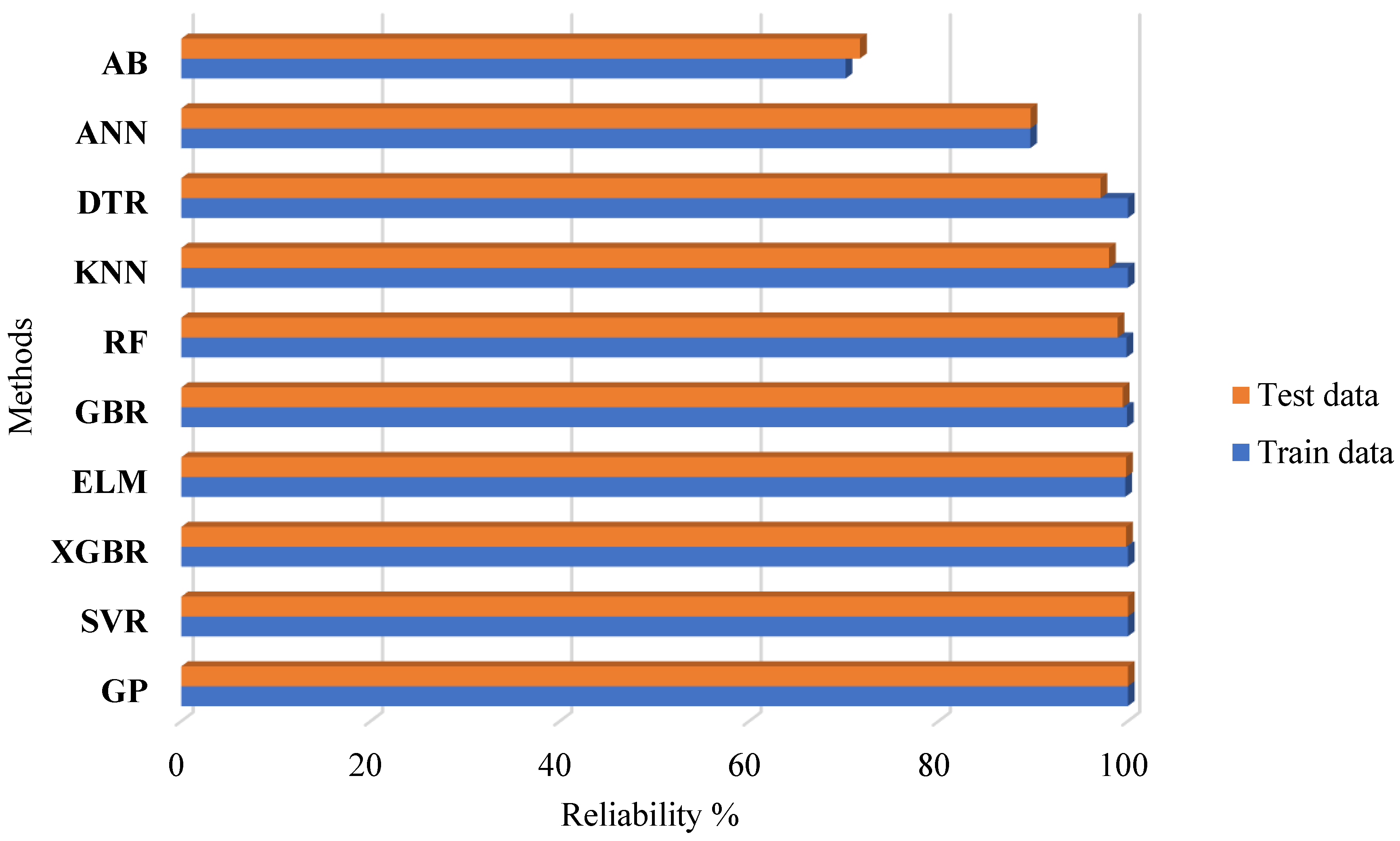
3.3. Results of the Reliability Analysis

Figure 9 displays the outcomes derived from the reliability analysis carried out on both the training and testing datasets. As shown, the x axis depicts the reliability percentages, while the y axis corresponds to the names of each estimation model. Regarding the reliability for the training dataset, most of the ML models exhibited exceptional performances. Specifically, the ELM, RF, and GBR models demonstrated robust reliability percentages exceeding 99%, while the GP, XGBR, SVR, KNN, and DTR models showed even higher performance levels at a perfect reliability of 100%. Conversely, the ANN and AB models yielded relatively weaker performances, with percentages of 89.69 and 70.19, respectively. On the other hand, the reliability of certain ML models, such as GP and SVR, remained equally robust for the testing dataset, achieving a reliability of 100%. The subsequent notable reliabilities were attained by the XGBR, ELM, GBR, RF, KNN, and DTR models, respectively. Although showing a perfect reliability of 100% for the training data, some ML models such as XGBR, KNN, and DTR indicated slightly lower reliability percentages of 99.82, 98.02, and 97.12, respectively, for the test data. Nevertheless, the ANN and AB models demonstrated relatively weaker reliability, with testing reliabilities of 89.73 and 71.71, respectively.

The outcomes of the reliability analysis were close to the metrics results, indicating the coherence and affirmation of the findings. The substantial reliability percentage observed in the employed models demonstrates their efficacy in forecasting WQI. Despite comparatively lower performance in certain ML models, like ANN and AB, compared with others, their reliability percentages remained adequate and satisfactory. Hence, the ML models exploited in this study acceptably captured relationships between input features and WQI.

Nowadays, there is a growing prevalence of the utilization of artificial intelligence and ML frameworks. The noteworthy outcomes demonstrated by such estimation models underscore their considerable potential. Researchers are advised to favor the application of such innovative approaches over traditional methodologies. Nevertheless, it is essential to recognize that each ML model possesses distinct merits and limitations. Thus, the accurate choice of an appropriate model tailored to the specific data of a given problem holds major significance. Additionally, it is crucial to emphasize that accurately tuning the hyperparameters of each model is essential to effectively model the problem at hand. Moreover, the field of programming is in a state of continuous evolution, giving rise to the introduction of advanced models. These newly introduced models may have the capacity to further augment the achieved results.

3.4. Discussion

According to the literature [15], the water quality status can be categorized into five distinct classes, which are as follows: (A) excellent, characterized by an WQI equal to or less than 50; (B) good, with an WQI ranging from 51 to 100; (C) poor, having an WQI in the range between 100 and 200; (D) very poor, with an WQI from 200 to 300; and finally, (E) unsuitable for drinking, indicated by an WQI exceeding 300. Analyzing a dataset comprising 2776 water quality observations for the Southern Bug River, it is evident that 51.19% of these observations fall within the excellent category, while 46.22% are in the category of good water quality. A smaller percentage, specifically 2.38%, belong to the poor water group, and a mere 0.21% fall below the poor water threshold. The WQI data overall illustrate that the river water quality is in a favorable condition.

This finding holds a greater significance when considering the vital role of the Southern Bug River within Ukraine, as it is one of the most significant and largest rivers in the country. In this regard, the WQI assessment plays a pivotal role in the river’s environmental and aquatic ecosystems to ensure water quality for various purposes. Moreover, the analysis of WQI not only contributes to regulatory compliance but also supports managing water resources. It can also function as an early warning system. Additionally, evaluating WQI facilitates the comprehension of the river’s dynamics and its broader environmental impact [16]. Hence, utilizing models for estimating WQI more precisely enables decision making and strategic planning for river management.

This study employed ten ML models to estimate WQI and assessed their predictive performances. Some models exhibited tendencies to overestimate or underestimate WQI values across different ranges, making them unsuitable as predictor models for forecasting the WQI of the Southern Bug River. According to the achieved results, the SVR and GP models showed exceptional correlations for both training and testing datasets, even though SVR had a slight underestimation for lower WQI values. Likewise, previous studies also showed the robust performance of SVR in estimating WQI [6,9,33]. Furthermore, Tiyasha et al. [10] provided a comprehensive survey encompassing over 200 studies from 2000 to 2020 focusing on the application of ML models in predicting river water quality. Their findings revealed that a substantial portion, i.e., 43%, of previous studies utilized ANN. As mentioned before, this approach gained considerable traction within the literature, displaying a commendable efficacy in forecasting WQI. Additionally, the study revealed that 10% of previous studies employed SVR, resulting in highly favorable outcomes. This finding further indicates the efficiency of SVR as a proficient tool for predicting WQI.

Performance metrics, including RMSE, MAE, MARE, MXARE, R², and NSE, were also computed for each model. While GP emerged as the most robust ML model based on the ranking scheme exploited in this study, XGBR showcased the second most commendable performance. This was consistent with the study by Khoi et al. [34], where they employed twelve ML models (AB, GBR, histogram-based GBR, light GBR, XGBR, DTR, extra trees, RF, MLP, radial basis function, deep feed-forward neural network, and convolutional neural network) to forecast WQI in a river in Vietnam. Their findings revealed that the XGBR model outperformed the others in terms of accuracy, whereas AB exhibited one of the weakest performances comparatively. Similarly, the AB model utilized in this study showed suboptimal results. Furthermore, Bui et al. [7] also concluded that AB exhibited comparatively less robust performance among the models they employed. Notably, RFR showed superior performance in predicting WQI in previous studies [7,11,29]. Finally, most of the ML models demonstrated satisfactory overall predictive abilities in the present study.

The reliability analysis results further supported the study findings, demonstrating robust performances for most models on both training and testing datasets, with some models achieving perfect reliability. The outcomes of this study underscore the potential of ML models for WQI estimations, emphasizing their advantages over traditional methods. Nonetheless, it is essential to acknowledge the significance of model selection and hyperparameter optimization, as evidenced by the relatively low reliability percentage observed in the case of AB. Application of AB for estimating WQI in the Southern Bug River may negatively impact river management projects. Moreover, the evolving field of ML techniques may introduce even more advanced models capable of improving results. Further investigations are encouraged to leverage these innovative approaches while carefully considering the specific characteristics of their data and the problem statement.

4. Conclusions

Forecasting of WQI for rivers is critical because it aids in identifying potential sources of pollution and the primary elements that markedly influence temporal and spatial fluctuations in river water quality. This study explored the potential of ten state-of-the-art ML techniques (SVR, DTR, RF, AB, GBR, XGBR, GP, ELM, ANN, and KNN) to predict WQI for the Southern Bug River in Ukraine. These ML-based models were developed on the data of nine physical and chemical parameters (NH4, BOD5, suspended solids, DO, NO₃, NO₂, SO₄, PO₄, and Cl) pertaining to a period of twenty-one years. The hyperparameters for each ML model implemented in this study were carefully fine-tuned to optimize their performances. The outcomes indicated strong correlations between predicted WQIs and observation-based ones for all ML models, excluding ANN and AB. Notably, GP and SVR demonstrated the most favorable estimations. Employing six statistical metrics showcased commendable performances across all ML models, despite relatively weaker results achieved by ANN and AB. To assess the ML models comprehensively, a ranking approach was adopted, revealing GP as the foremost estimation model, trailed by XGBR, SVR, KNN, GBR, ELM, DTR, RF, ANN, and AB. Eight out of ten ML models performed so well that, while KNN excelled for the training data, a marginal decline for the testing data led to a seventh-place ranking in testing and a joint third overall position alongside SVR. For ANN and AB, lower metrics across the datasets positioned them as the last two models. Reinforcing prior findings, a reliability assessment indicated 100% reliability for GP, SVR, and XGBR, with AB displaying slightly over 70% reliability. In summary, eight out of ten ML models exhibited exceptional WQI prediction performances, while the remaining two displayed satisfactory performances with reliability surpassing 70%. These results underscore the robust utility of ML models in water quality management, offering valuable support to hydraulic engineers.

In future studies, the efficacy of the applied models can be improved by incorporating other important parameters as per WHO guidelines. In addition, performances of ML models can be evaluated across various global rivers characterized by distinct climatic and hydrological contexts.

References

1. Alam, J.B.; Islam, M.R.; Muyen, Z.; Mamun, M.; Islam, S. Archive of SID Water quality parameters along rivers Archive of SID. Int. J. Environ. Sci. Technol. 2007, 4, 159–167. [Google Scholar] [CrossRef]
2. Khan, I.; Zakwan, M.; Mohanty, B. Water Quality Assessment for Sustainable Environmental Management. ECS Trans. 2022, 107, 10133. [Google Scholar] [CrossRef]
3. Alizamir, M.; Sobhanardakani, S. An Artificial Neural Network—Particle Swarm Optimization (ANN- PSO) Approach to Predict Heavy Metals Contamination in Groundwater Resources. Jundishapur J. Health Sci. 2018, 10, e67544. [Google Scholar] [CrossRef]
4. Ghobadi, A.; Cheraghi, M.; Sobhanardakani, S.; Lorestani, B.; Merrikhpour, H. Hydrogeochemical characteristics, temporal, and spatial variations for evaluation of groundwater quality of Hamedan–Bahar Plain as a major agricultural region, West of Iran. Environ. Earth Sci. 2020, 79, 428. [Google Scholar] [CrossRef]
5. Khan, I.; Zakwan, M.; Pulikkal, A.K.; Lalthazula, R. Impact of unplanned urbanization on surface water quality of the twin cities of Telangana state, India. Mar. Pollut. Bull. 2022, 185, 114324. [Google Scholar] [CrossRef]
6. Haghiabi, A.H.; Nasrolahi, A.H.; Parsaie, A. Water quality prediction using machine learning methods. Water Qual. Res. J. 2018, 53, 3–13. [Google Scholar] [CrossRef]
7. Bui, D.T.; Khosravi, K.; Tiefenbacher, J.; Nguyen, H.; Kazakis, N. Improving prediction of water quality indices using novel hybrid machine-learning algorithms. Sci. Total Environ. 2020, 721, 137612. [Google Scholar] [CrossRef] [PubMed]
8. El Bilali, A.; Taleb, A. Prediction of irrigation water quality parameters using machine learning models in a semi-arid environment. J. Saudi Soc. Agric. Sci. 2020, 19, 439–451. [Google Scholar] [CrossRef]
9. Aldhyani, T.H.H.; Al-Yaari, M.; Alkahtani, H.; Maashi, M. Water Quality Prediction Using Artificial Intelligence Algorithms. Appl. Bionics Biomech. 2020, 2020, 6659314. [Google Scholar] [CrossRef]
10. Tiyasha; Tung, T.M.; Yaseen, Z.M. A survey on river water quality modelling using artificial intelligence models: 2000–2020. J. Hydrol. 2020, 585, 124670. [Google Scholar] [CrossRef]
11. Kouadri, S.; Elbeltagi, A.; Islam, A.R.M.T.; Kateb, S. Performance of machine learning methods in predicting water quality index based on irregular data set: Application on Illizi region (Algerian southeast). Appl. Water Sci. 2021, 11, 190. [Google Scholar] [CrossRef]
12. Asadollah, S.B.H.S.; Sharafati, A.; Motta, D.; Yaseen, Z.M. River water quality index prediction and uncertainty analysis: A comparative study of machine learning models. J. Environ. Chem. Eng. 2021, 9, 104599. [Google Scholar] [CrossRef]
13. Ahmed, M.; Mumtaz, R.; Anwar, Z.; Shaukat, A.; Arif, O.; Shafait, F. A multi–step approach for optically active and inactive water quality parameter estimation using deep learning and remote sensing. Water 2022, 14, 2112. [Google Scholar] [CrossRef]
14. Uddin, M.G.; Nash, S.; Rahman, A.; Olbert, A.I. Performance analysis of the water quality index model for predicting water state using machine learning techniques. Process Saf. Environ. Prot. 2023, 169, 808–828. [Google Scholar] [CrossRef]
15. Goodarzi, M.R.; Niknam, A.R.R.; Barzkar, A.; Niazkar, M.; Zare Mehrjerdi, Y.; Abedi, M.J.; Heydari Pour, M. Water Quality Index Estimations Using Machine Learning Algorithms: A Case Study of Yazd-Ardakan Plain, Iran. Water 2023, 15, 1876. [Google Scholar] [CrossRef]
16. Shakhman, I.; Bystriantseva, A. Water Quality Assessment of the Surface Water of the Southern Bug River Basin by Complex Indices. J. Ecol. Eng. 2020, 22, 195–205. [Google Scholar] [CrossRef]
17. Frank, A.J. UCI Machine Learning Repository. 2010. Available online: http://archive.ics.uci.edu/ml (accessed on 1 January 2023).
18. Das Kangabam, R.; Bhoominathan, S.D.; Kanagaraj, S.; Govindaraju, M. Development of a water quality index (WQI) for the Loktak Lake in India. Appl. Water Sci. 2017, 7, 2907–2918. [Google Scholar] [CrossRef]
19. Ismail, A.H.; Robescu, D. Assessment of water quality of the Danube river using water quality indices technique. Environ. Eng. Manag. J. 2019, 18, 1727–1737. [Google Scholar] [CrossRef]
20. Pesce, S.F.; Wunderlin, D.A. Use of Water Quality Indices To Verify the Córdoba City (Argentina) on Suquía River. Wat. Res. 2000, 34, 2915–2926. [Google Scholar] [CrossRef]
21. Cotruvo, J.A. 2017 Who guidelines for drinking water quality: First addendum to the fourth edition. J. Am. Water Work. Assoc. 2017, 109, 44–51. [Google Scholar] [CrossRef]
22. Gaya, M.S.; Abba, S.I.; Abdu, A.M.; Tukur, A.I.; Saleh, M.A.; Esmaili, P.; Wahab, N.A. Estimation of water quality index using artificial intelligence approaches and multi-linear regression. IAES Int. J. Artif. Intell. 2020, 9, 126–134. [Google Scholar] [CrossRef]
23. Gazzaz, N.M.; Yusoff, M.K.; Aris, A.Z.; Juahir, H.; Ramli, M.F. Artificial neural network modeling of the water quality index for Kinta River (Malaysia) using water quality variables as predictors. Mar. Pollut. Bull. 2012, 64, 2409–2420. [Google Scholar] [CrossRef] [PubMed]
24. Gupta, R.; Singh, A.N.; Singhal, A. Application of ANN for water quality index. Int. J. Mach. Learn. Comput. 2019, 9, 688–693. [Google Scholar] [CrossRef]
25. Yıldız, S.; Karakuş, C.B. Estimation of irrigation water quality index with development of an optimum model: A case study. Environ. Dev. Sustain. 2020, 22, 4771–4786. [Google Scholar] [CrossRef]
26. Piraei, R.; Afzali, S.H.; Niazkar, M. Assessment of XGBoost to Estimate Total Sediment Loads in Rivers. Water Resour. Manag. 2023. [Google Scholar] [CrossRef]
27. Piraei, R.; Niazkar, M.; Afzali, S.H.; Menapace, A. Application of Machine Learning Models to Bridge Afflux Estimation. Water 2023, 15, 2187. [Google Scholar] [CrossRef]
28. Ebtehaj, I.; Bonakdari, H.; Moradi, F.; Gharabaghi, B.; Khozani, Z.S. An integrated framework of Extreme Learning Machines for predicting scour at pile groups in clear water condition. Coast. Eng. 2018, 135, 1–15. [Google Scholar] [CrossRef]
29. Anmala, J.; Turuganti, V. Comparison of the performance of decision tree (DT) algorithms and extreme learning machine (ELM) model in the prediction of water quality of the Upper Green River watershed. Water Environ. Res. 2021, 93, 2360–2373. [Google Scholar] [CrossRef]
30. Alomar, M.K.; Khaleel, F.; Aljumaily, M.M.; Masood, A.; Razali, S.F.M.; AlSaadi, M.A.; Al-Ansari, N.; Hameed, M.M. Data-driven models for atmospheric air temperature forecasting at a continental climate region. PLoS ONE 2022, 17, e0277079. [Google Scholar] [CrossRef]
31. Schulz, E.; Speekenbrink, M.; Krause, A. A tutorial on Gaussian process regression: Modelling, exploring, and exploiting functions. J. Math. Psychol. 2018, 85, 1–16. [Google Scholar] [CrossRef]
32. Niazkar, M.; Zakwan, M. Developing ensemble models for estimating sediment loads for different times scales. Environ. Dev. Sustain. 2023. [Google Scholar] [CrossRef]
33. Mohammadpour, R.; Shaharuddin, S.; Chang, C.K.; Zakaria, N.A.; Ghani, A.A.; Chan, N.W. Prediction of water quality index in constructed wetlands using support vector machine. Environ. Sci. Pollut. Res. 2015, 22, 6208–6219. [Google Scholar] [CrossRef] [PubMed]
34. Khoi, D.N.; Quan, N.T.; Linh, D.Q.; Nhi, P.T.T.; Thuy, N.T.D. Using machine learning models for predicting the water quality index in the La Buong River, Vietnam. Water 2022, 14, 1552. [Google Scholar] [CrossRef]
Figure 1. Location of the Southern Bug River.
Water 15 03543 g001
Figure 2. Typical Structure of an ELM.
Water 15 03543 g002
Figure 3. Random Forest prediction process.
Water 15 03543 g003
Figure 4. SVMs Optimize Margins Between Support Vectors or Classes. Colorful shapes are the classified data points.
Water 15 03543 g004
Figure 5. Modelling process of the ML models adopted in this study.
Water 15 03543 g005
Figure 6. Comparison of estimated values with observations for the training dataset.
Water 15 03543 g006
Figure 7. Comparison of estimated values with observations for the testing dataset.
Water 15 03543 g007
Figure 8. Heat maps of the metrics results for both training and testing datasets.
Water 15 03543 g008
Figure 9. Reliability results.
Water 15 03543 g009