Abstract
Accurate predictions of future climate change are significant to both human social production and development. Accordingly, the changes in the daily maximum (Tmax) and minimum temperatures (Tmin) in the Yarlung Tsangpo-Brahmaputra River Basin (YBRB), along with its three sub-regions (Tibetan Plateau—TP, Himalayan Belt—HB, and Floodplain—FP) were evaluated here using the Bayesian model average (BMA) results from nine climate models in the CMIP6 under four future scenarios, and the corresponding uncertainty of the projected results was analyzed. The results showed the following: (1) The BMA can simulate the Tmax and Tmin of the YBRB well. (2) Future Tmax and Tmin over the YBRB exhibited an overall fluctuating upward trend. Even under the most ideal sustainable development scenario examined (SSP126), the average Tmax (Tmin) over the YBRB was projected to increase by 3.53 (3.38) °C by the end of this century. (3) Although the future changes in the YBRB are predicted to fall below the global average, the future temperature difference in the YBRB will increase further. (4) The uncertainty increased with prediction time, while spatially, the regions with the uncertainty were the TP > HB > FP. These findings can provide a reference for the YBRB climate change adaptation strategies.
1. Introduction
Global climate change is increasingly accepted as fact, as the Sixth Assessment Report of the United Nations Intergovernmental Panel on Climate Change (IPCC) has confirmed that the average global surface temperature in the first two decades of the 21st century (2001–2020) increased by 0.99 °C relative to the global surface temperature during the Industrial Revolution (1850–1900) [1]. Under warmer global temperatures, certain natural disasters (storms, floods, heatwaves, droughts, and fires) are expected to occur more frequently [2,3], significantly impacting agriculture, social economy, human well-being, etc. [4,5,6,7,8], and potentially increasing global conflicts [9,10]. Similar to other parts of the world, significant warming has been observed on and around the Tibetan Plateau in recent decades. Studies have shown that the increased melting of glaciers and snow cover caused by warming in this Third Polar Region will continue to threaten water supply security throughout Asia [11,12]. Daily maximum (Tmax) and minimum temperatures (Tmin) are fundamental metrics in climate change research and important indicators of extreme climate events. Accordingly, reasonable assessments of future Tmax and Tmin values are beneficial for predicting the impact of extreme climate events across all sectors, informing national climate policies, as well as maintaining the stability of regional ecosystems and socioeconomic development.
Global climate models are important tools for climate science research [13,14], capable of explaining past climate change and predicting future climate [15]. Since 1995, the Working Group on Coupled Models of the World Climate Research Programme has initiated and organized six Coupled Model Intercomparison Projects. The Coupled Model Intercomparison Project (CMIP) seeks to better understand past, present, and future climate changes caused by natural, unforced, or radiative forcing in multi-model environments [16]. Since its inception, the CMIP has made significant contributions to various IPCC assessment reports [1,17,18,19]. Elsewhere, Song et al. [20] used 20 climate models from the Fifth Coupled Model Intercomparison Project (CMIP5) to predict warmer global surface air temperatures under higher emission scenarios. Zhao et al. [21] employed the CMIP5 multi-model to simulate climate change across typical arid and semi-arid regions of the world, revealing the stronger capacity of the multi-model ensemble (MME) mean compared to any individual model. However, one of the important problems is that there are large uncertainties in using global climate models for the prediction or projection of future climate. Multi-model weighting based on performance indicators has been found to reduce the uncertainty of predicted results [22,23,24,25,26,27,28]. Specifically, Bayesian model averaging (BMA) has been shown to be less uncertain than either single model or MME results [29,30,31].
The Yarlung Tsangpo-Brahmaputra River is an important international river in Asia, which spans multiple countries (China, India, Bhutan, and Bangladesh), and maintains great potential for hydropower along with other abundant water resources. The geography of the Yarlung Tsangpo-Brahmaputra River Basin (YBRB) is diverse, the climate is complex, and climate change has already had a significant impact on the local hydrology and ecology. Accordingly, predicting future regional climate change across the YBRB is of great significance to all countries in the basin [32]. So far, The YBRB has been partially studied regarding climate change. Shi et al. [33] used a high-resolution regional climate model (RegCM3) simulation to study future climate change under the A1B scenario of the IPCC Special Report on Emissions Scenarios. Immerzeel [34] predicted future YBRB temperature, precipitation, and hydrological cycles using six climate model datasets (2002–2100) under two scenarios via a multiple linear regression model. The CMIP has entered its sixth phase (CMIP6), characterized by higher spatial resolution models, improved physical parameterization schemes, as well as new Earth system processes and components [16,35,36]; yet, the basin-scale study of the YBRB under CMIP6 remains lacking.
Accordingly, this study conducted the following work in the YBRB using the most common CMIP6 climate model data. Based on historical data (1961–2014), a Bayesian model was trained, and the BMA’s ability to simulate the Tmax and Tmin over the YBRB test period (2005–2014) was evaluated. Each model was evaluated according to the weight coefficient obtained during the optimal training period. Based on the observational data and BMA prediction results, the changing trends of the Tmax and Tmin in the YBRB historical (1961–2014) and future periods (2015–2100) were acquired. Additionally, the changing trend and increase in the Tmax and Tmin of the YBRB were discussed over different periods. Lastly, the quantitative uncertainty of the predicted results was discussed to provide a scientific basis for the YBRB climate change adaptation strategies and decision making.
2. Materials and Methods
2.1. Study Area
The Yarlung Tsangpo-Brahmaputra River spans 2900 km in China, India, Bhutan, and Bangladesh, comprising a drainage area of 53,000 km2 [37,38]. It originates from the Jamayangzong Glacier in Tibet, and its upstream region is the Yarlung Tsangpo River. It is the fifth largest river in China and the highest river in the world, with an average altitude > 4000 m. After entering India, the river is known as the Brahmaputra River; within the territory of Bangladesh, it joins with the Ganges and the Jamuna River and flows into the Bay of Bengal [32]. The seasonal distribution of precipitation within the YBRB is highly uneven, with the period from June to September accounting for 60%–70% of the total annual precipitation [39]. Furthermore, heavy and concentrated precipitation events lead to frequent flooding in the lower YBRB [40]. The majority of monthly mean Tmax values are recorded in June–July; whereas monthly mean Tmin occur in December–January. Annual temperature differences can be as high as 40 °C, with a strong differential between the upper and lower reaches, and obvious vertical changes [41]. There are 10 different climate types within the YBRB which vary significantly by region. The overall pattern—dry and cold on the plateau, dry and hot in the mountains, and warm and wet on the plains—is strongly influenced by the division of the Himalayas [42,43].
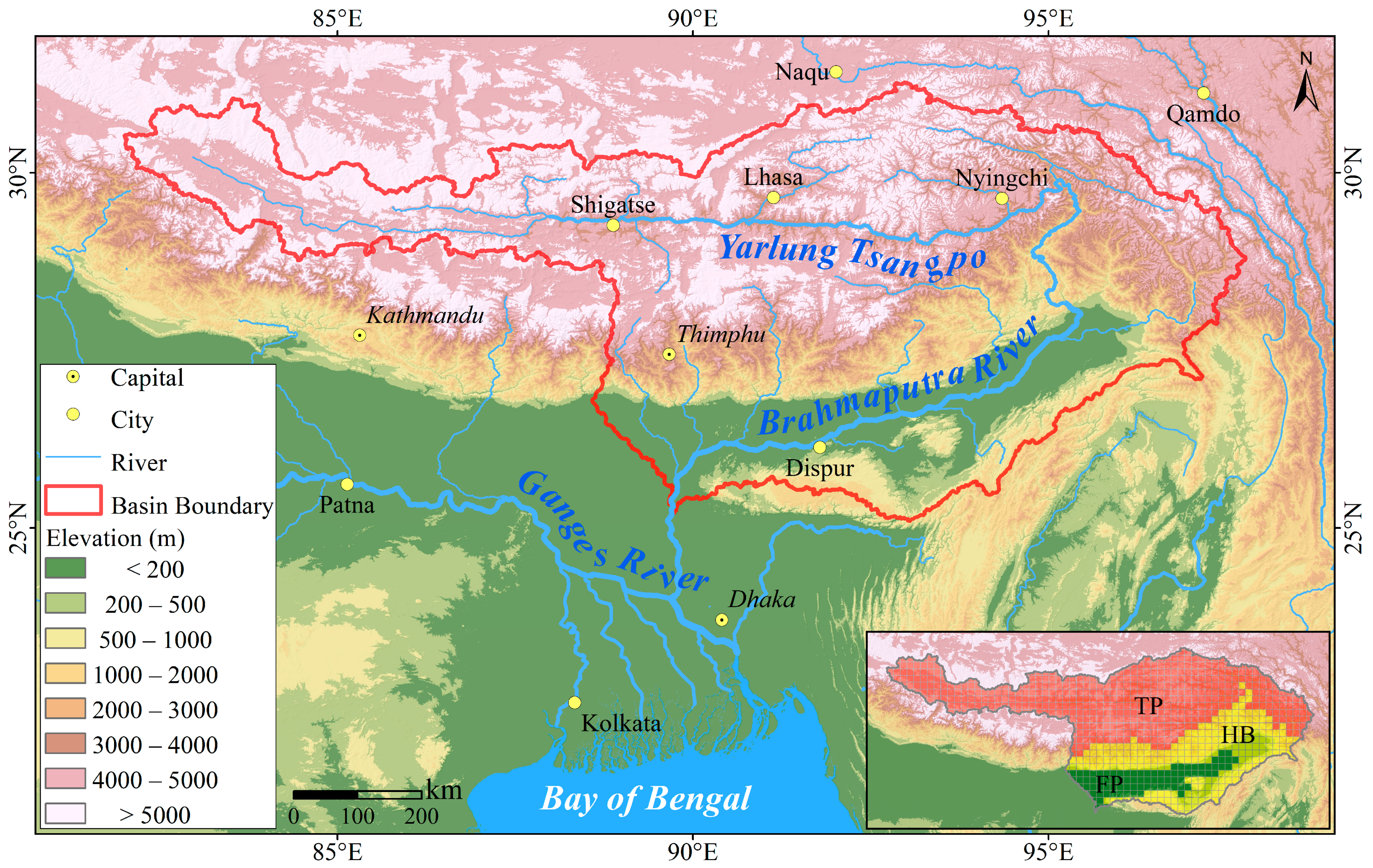
Considering the vast territory and substantial topographic differences across the YBRB, the simulation effects of climate models vary regionally. In accordance with the physical geographical zoning method of Immerzeel [34], this study divided the YBRB into three sub-regions for spatial analysis: the Tibetan Plateau (TP, elevation ≥ 3500 m), the Himalayan Belt (HB, elevation 100~3500 m), and the Floodplain (FP, elevation ≤ 100 m; Figure 1).
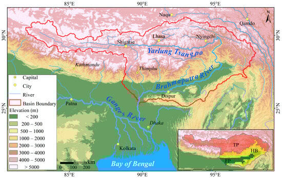
Figure 1.
Map of Yarlung Tsangpo-Brahmaputra River Basin (YBRB): TP—Tibetan Plateau, HB—Himalayan Belt, and FP—Floodplain.
2.2. Materials
Based on the availability of the CMIP6 climate model data and its frequency of use (Table S1), nine climate model data sets were selected under four shared socioeconomic pathway (SSP) scenarios: SSP126, SSP245, SSP370, and SSP585 (see O’Neill et al. [44] for further background on SSPs). Table 1 shows the basic information of the selected 9 models, with greater detail listed on the CMIP6 website (https://esgf-node.llnl.gov/projects/cmip6/. Accessed on 15 May 2022). The selected climate model data included daily Tmax and Tmin data from the historical climate simulation experiment (1961–2014) and future emission scenario experiment (2015–2100). Owing to differences in the spatial resolution among the climate models, the bilinear interpolation method was used to resample all the model resolutions to 0.25° × 0.25° [45,46]. Reference daily observation data from the historical period were used with the bias-corrected PGF-V3 (Princeton Global Forcings) Tmax and Tmin data from Ji et al. [47]. The PGF-V3 dataset coverage maintained a similar resolution (0.25° × 0.25°) and was sufficiently long for inclusion in the present study (1948–2016) [47].

Table 1.
Basic information of the 9 CMIP6 climate models.
2.3. BMA Estimation
The BMA method was used here to fuse the CMIP6 multi-model data (daily Tmax and Tmin) for predicting future temperature changes across the YBRB and evaluating its uncertainty. In contrast to a single optimal model, the BMA assigns a weight to each model and determines the final predicted value using the weighted average, thereby producing more reliable predicted values. An average BMA forecast can be calculated via Equation (1):
where y is the predicted variable, is the th model prediction, and means the corresponding conditional probability density function. When the study variable is temperature, approximately follows a normal distribution with an expectation of [29]. If the variable has not yet been bias-corrected, can be seen as a simple bias correction process, and can also be considered as a simple form of model output statistics [48,49]. and can be obtained using a linear regression. can be obtained using the maximum likelihood estimation principle [50] and expectation maximization algorithm [51] alongside the training period dataset. Further details about the BMA method can be found in Raftery et al. [29].
Lastly, the BMA future estimate is calculated using Equation (2):
where is the mean temperature change of the th model over the next 20 years compared to the reference period (1995–2014).
2.4. Evaluation Metrics of Ensemble Mean
The root mean square error (RMSE) and anomaly correlation coefficient (ACC) were used to test the BMA simulation results. The RMSE was used to measure the deviation between the simulated and real values: the smaller the RMSE value, the better the BMA simulation effect (Equation (3)):
where is the total amount of data obtained, is the BMA simulation result, and is the observed value.
Alternatively, ACC also represents the degree of similarity between the simulated and observed value, with a greater correlation coefficient indicating a stronger relationship (Equation (4)):
where is the average BMA simulation result value, and is the observational average.
2.5. Uncertainty Estimation
Pennell and Reichler [52] found that multi-model weighting results are dependent upon the modes that comprise the modal set (i.e., the effective modes); therefore, the effective mode number () was introduced into the calculation of the difference between modes (Equations (5) and (6)):
The model interval deviation can be used to characterize the uncertainty of BMA results, where the greater the value, the higher the uncertainty and lower the reliability of the predicted result.
2.6. Determine the Optimal Training Period
When constructing a Bayesian model, it is necessary to divide historical multi-model and observation data series into training and test periods, and evaluate the overall effects on the latter to select the optimal model. Here, different training period lengths were explored, and the performance of the model was judged based on the RMSE and ACC between the BMA estimate and test period observations. Finally, 28 and 20 years were selected as the optimal training periods for the Tmax and Tmin, respectively (see Text S1 in Supporting Information).
3. Results and Discussion
3.1. Evaluation of BMA Simulation
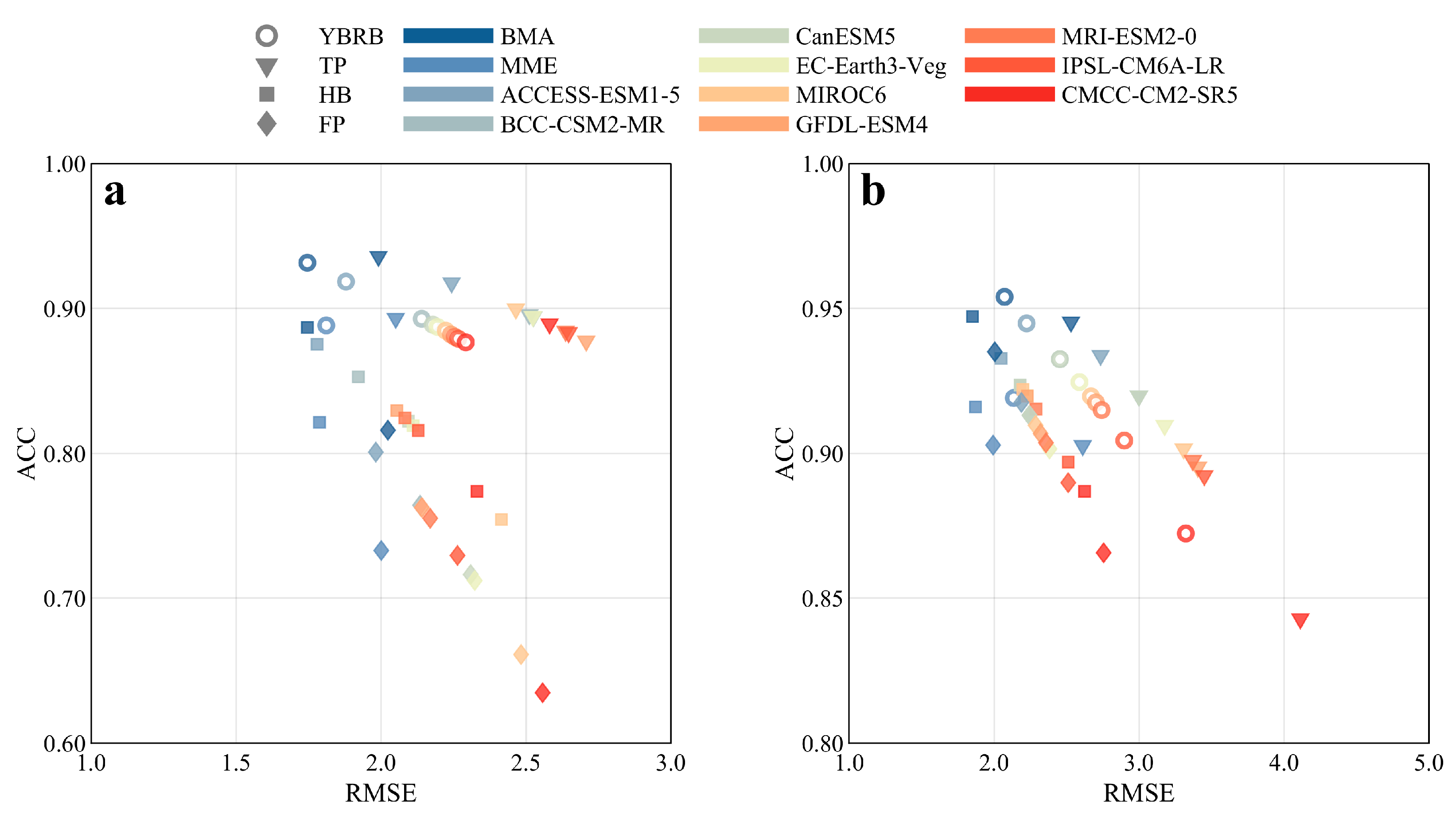
The performances of the Tmax and Tmin simulated by the optimal BMA model in the YBRB were evaluated and compared with those of the MME and single model (Figure 2, the closer it is to the top right corner, the better the simulation).

Figure 2.
RMSE and ACC between BMA, MME, 9 climate model projections and observations of Tmax (a), Tmin (b) in the YBRB and its accompanying sub-regions during 2005–2014.
The RMSE of the BMA-simulated Tmax over the YBRB was 1.75 °C, notably lower than that of the MME or the nine single models (1.81–2.29 °C; Figure 2a). The higher ACC of the Tmax simulated by the BMA for the YBRB (0.93) compared to that of the MME and nine single models (0.88–0.92) further supported its predictive superiority. By sub-region, the Tmax RMSE for the TP and HB simulated by the BMA were 1.99 °C and 1.75 °C, respectively, lower than that of the MME and nine single models (TP: 2.05–2.71 °C, HB:1.78–2.41 °C). Comparatively, the Tmax RMSE for the FP simulated by the BMA (2.02 °C) was slightly larger than that of the MME (2.00 °C) and CanESM5 (1.98 °C), but smaller than that of the other eight models (2.13–2.56 °C). The Tmax ACC for the TP, HB, and FP simulated by the BMA were 0.94, 0.89, and 0.82, respectively, higher than those of the MME and nine models (TP: 0.88–0.92, HB: 0.76–0.88, FP: 0.63–0.80). By comparing the performances across the three regions, it was revealed that the Tmax simulated by the BMA was better in the HB than in the TP or FP.
The RMSE of the Tmin simulated by the BMA for the YBRB was 2.07 °C, lower than that of the MME and the nine models (2.13–3.32 °C); the ACC of the Tmin simulated by the BMA for the YBRB (0.95) was also higher than that of the MME or the nine single models (0.87–0.94; Figure 2b). By sub-region, the Tmin RMSE for the TP and HB simulated by the BMA was 2.53 °C and 1.85 °C, respectively, lower than those of the MME and nine models (TP: 2.61–4.11 °C, HB: 1.87–2.62 °C). The BMA-derived ACC of the Tmin (2.00 °C) was slightly larger than that of the MME (1.99 °C), but less than that of the other nine models (2.19–2.76 °C). By region, the ACC of the Tmin for the TP, HB, and FP were 0.95, 0.95, and 0.94, respectively, greater than that of the MME and the nine models (TP: 0.84–0.93, HB: 0.89–0.93, FP: 0.87–0.92). Ultimately, when comparing the performance of the overall region and different sub-regions, the Tmin values simulated by the BMA were superior to the MME and the other individual models, particularly over the TP and FP compared to the HB region (consistent with the Tmax).
In general, the BMA effectively improved the climate model predictions of the Tmax and Tmin over the YBRB; thus, the BMA-based CMIP6 multi-model set was recommended for future Tmax and Tmin change predictions across this region.
3.2. Evaluation of Weighted Model Performance
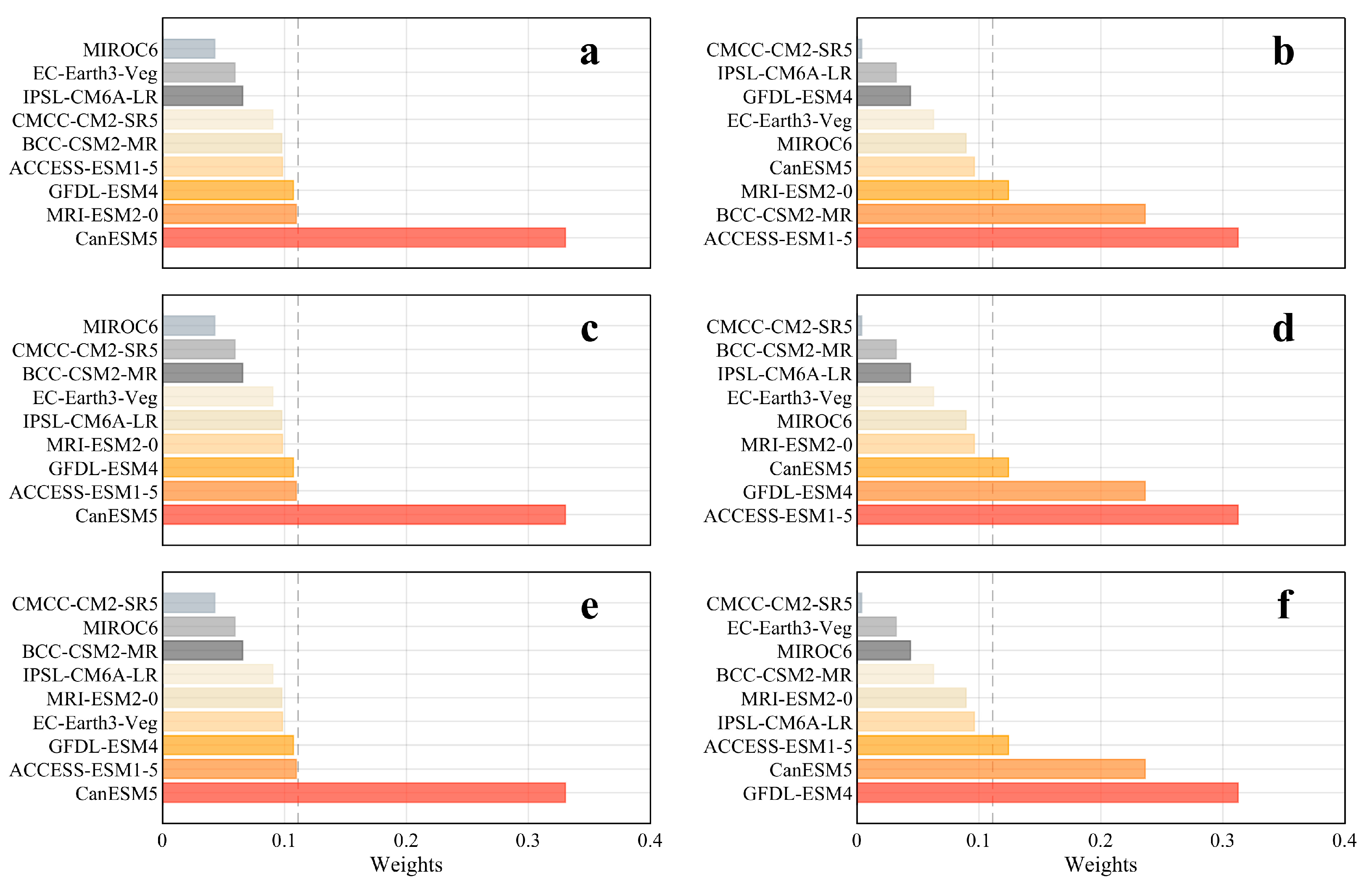
Model weights reflect their relative contribution to the ensemble average results during the training period, where increased weights equate to each model’s stronger forecasting ability. Figure 3 shows the weight distribution comparison for the nine climate model components across each YBRB sub-region throughout the optimal training period. For Tmax, the top three climate model results were CanESM5 > ACCESS-ESM1-5 > GFDL-ESM4 among the three sub-regions. The average weight of the three sub-regions was ≥ 0.35, far exceeding the equal weight value of 0.11. Comparatively, the worst-performing model was MIROC6, with sub-equal weights across all three sub-regions of the YBRB, averaging ≥ 0.02. The top Tmin simulation models were ACCESS-ESM1-5 > GFDL-ESM4 > MRI-ESM2-0. For ACCESS-ESM1-5, the weights of the TP (0.27) and HB (0.25) reached their maximum values, far exceeding the equal weight of 0.11; however, the simulation effect on the FP was relatively poor (0.14; GFDL-ESM4 was the top-performing model for the FP). For Tmin, the poorest performing model was CMC-CM2-SR5, with all sub-region weights lower than the equal weights (averaging ≥ 0.01).
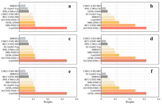
Figure 3.
Weight distribution of 9 climate models across different regions (TP: (a,b); HB: (c,d); FP: (e,f)) of the YBRB during the optimal training period (dashed lines depict equal weights): left column (Tmax), right column (Tmin).
Namely, the ACCESS-ESM1-5 and CanESM5 models performed the best for Tmax and Tmin over the YBRB; whereas CMC-CM2-SR5 produced the poorest simulation effects. For the performance of ACCESS-ESM1-5, Lun et al. [53] evaluated the ability of 24 CMIP6 climate models to simulate the TP temperature, also revealing the superiority of ACCESS-ESM1-5. It indicated that the ACCESS-ESM1-5 should be preferred when the CMIP6 model is used to study the temperature, Tmax and Tmin of the TP and its surrounding areas. In addition, the same climate model produced distinct simulation effects across different variables, such as Tmax and Tmin. Zhu and Yang [54] used CMIP5 and CMIP6 data to simulate historical TP temperatures and precipitation, and found that the same climate model had different simulation effects on temperatures and precipitation. Hence, it is advisable to assess climate models specifically for the study area and variables when selecting them.
3.3. Spatiotemporal Distribution of Future YBRB Temperature Changes
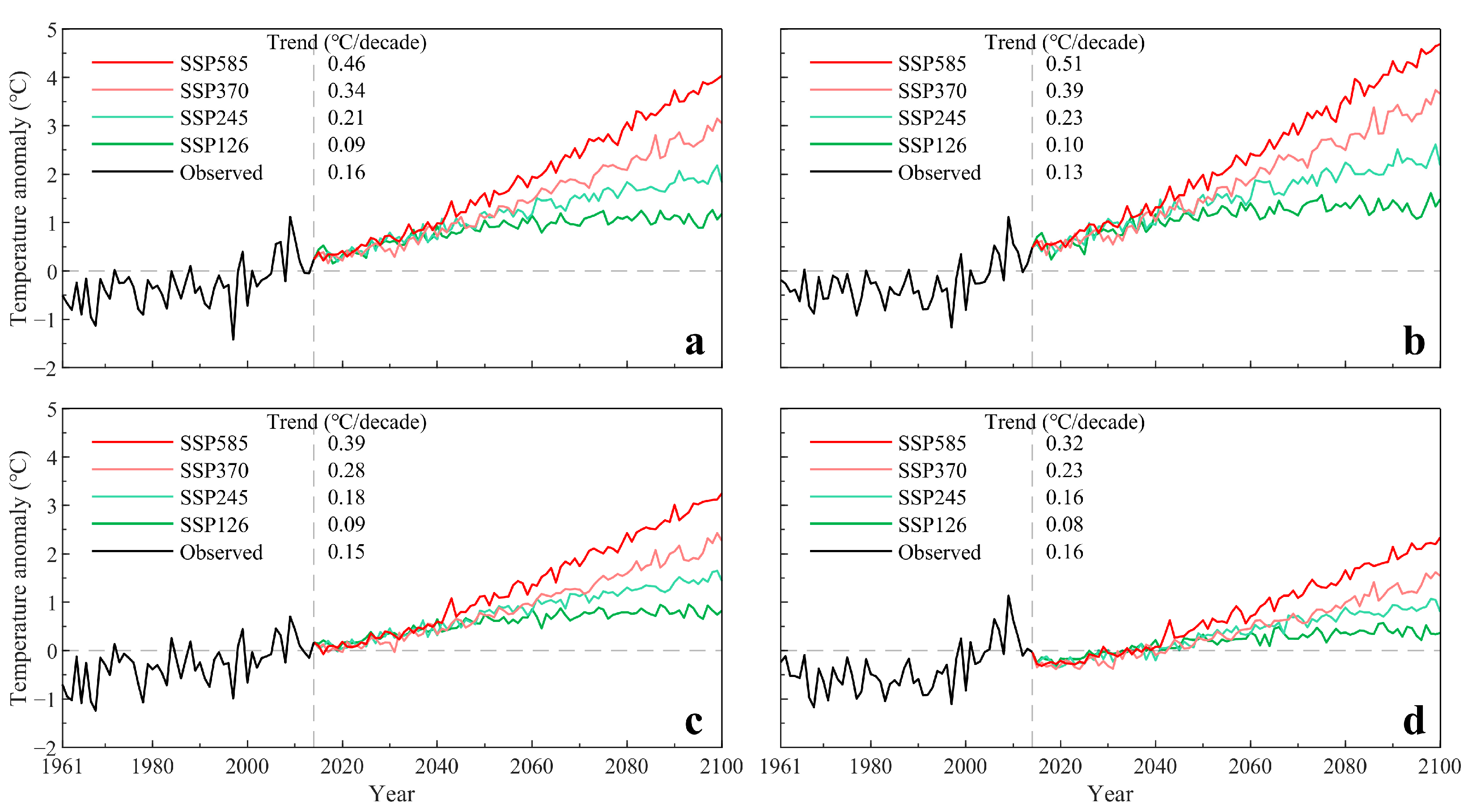
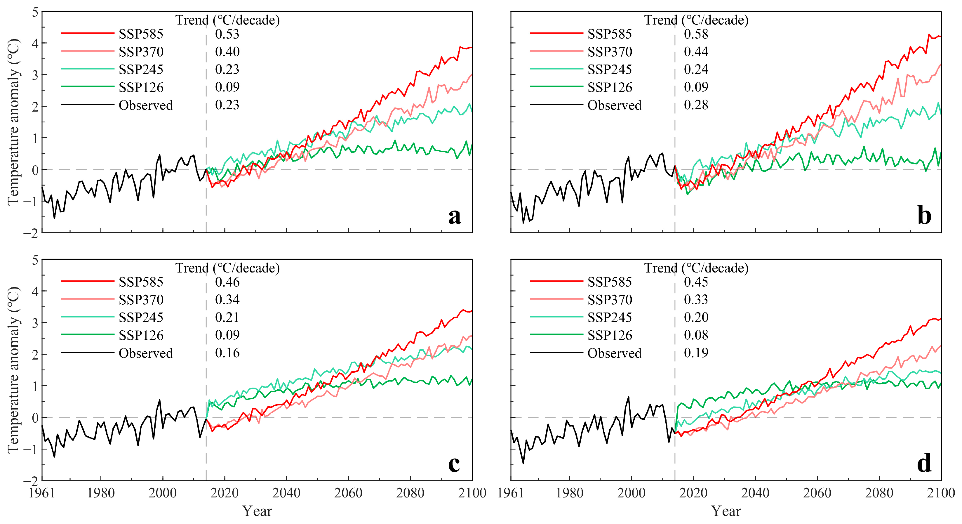
According to the principle of the BMA method, the expected maximization algorithm can be used to obtain the estimated values of each model parameter throughout the optimal training period. To this end, the BMA-projected Tmax and Tmin values for the future period (2015–2100) were calculated via Equation (1). In accordance with the IPCC Sixth Assessment Report, the future period was divided into the near- (2021–2040), mid- (2041–2060), and long-term (2081–2100) [1]. Figure 4 and Figure 5 reflect the overall change trends of the annual mean Tmax and Tmin across the YBRB, respectively, as projected by the BMA under different climate scenarios. Over the period from 2015 to 2100, the growth rate of the BMA-predicted Tmin under the SSP245, SSP370, and SSP585 scenarios was higher than that of the Tmax; whereas these rates were similar in the SSP126 emission scenario. When comparing the growth rates of different sub-regions, it was found that the future Tmax and Tmin growth rates predicted by the BMA showed similar characteristics under the four scenarios; that is, the fastest growing region was the TP, followed by the HB and the FP. This finding further corroborates the discovery made by Immerzeel [34], which indicates that the growth rate of future YBRB temperatures exhibits significant spatial variations, with higher regional altitudes experiencing faster temperature growth. It was also found that the increase in the development scenario intensity led to stronger growth rates of Tmax over the YBRB throughout the 21st century, with these differences becoming more extrapolated towards the latter end of this era (Figure 4). For Tmin, the rate of increase did not particularly increase with the development scenario intensities until the mid- and long-term periods (Figure 5).
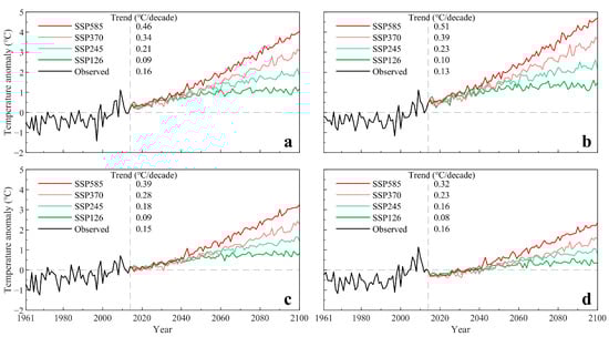
Figure 4.
Time series of annual surface Tmax from the BMA of 9 CMIP6 models over the YBRB (a) and its three sub-regions (TP: (b); HB: (c); FP: (d)) during 1961–2100 relative to 1961–2014 under SSP126, SSP245, SSP370, and SSP585. Trends were calculated for 19612014 observations, as well as SSP126, SSP245, SSP370, and SSP585 during 2015–2100.
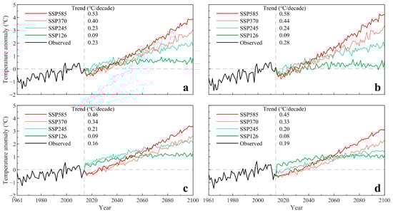
Figure 5.
Time series of annual surface Tmin from the BMA of 9 CMIP6 models over the YBRB (a) and its three sub-regions (TP: (b); HB: (c); FP: (d)) during 1961–2100 relative to 1961–2014 under SSP126, SSP245, SSP370, and SSP585. Trends were calculated for 1961–2014 observations, as well as SSP126, SSP245, SSP370, and SSP585 during 2015–2100.
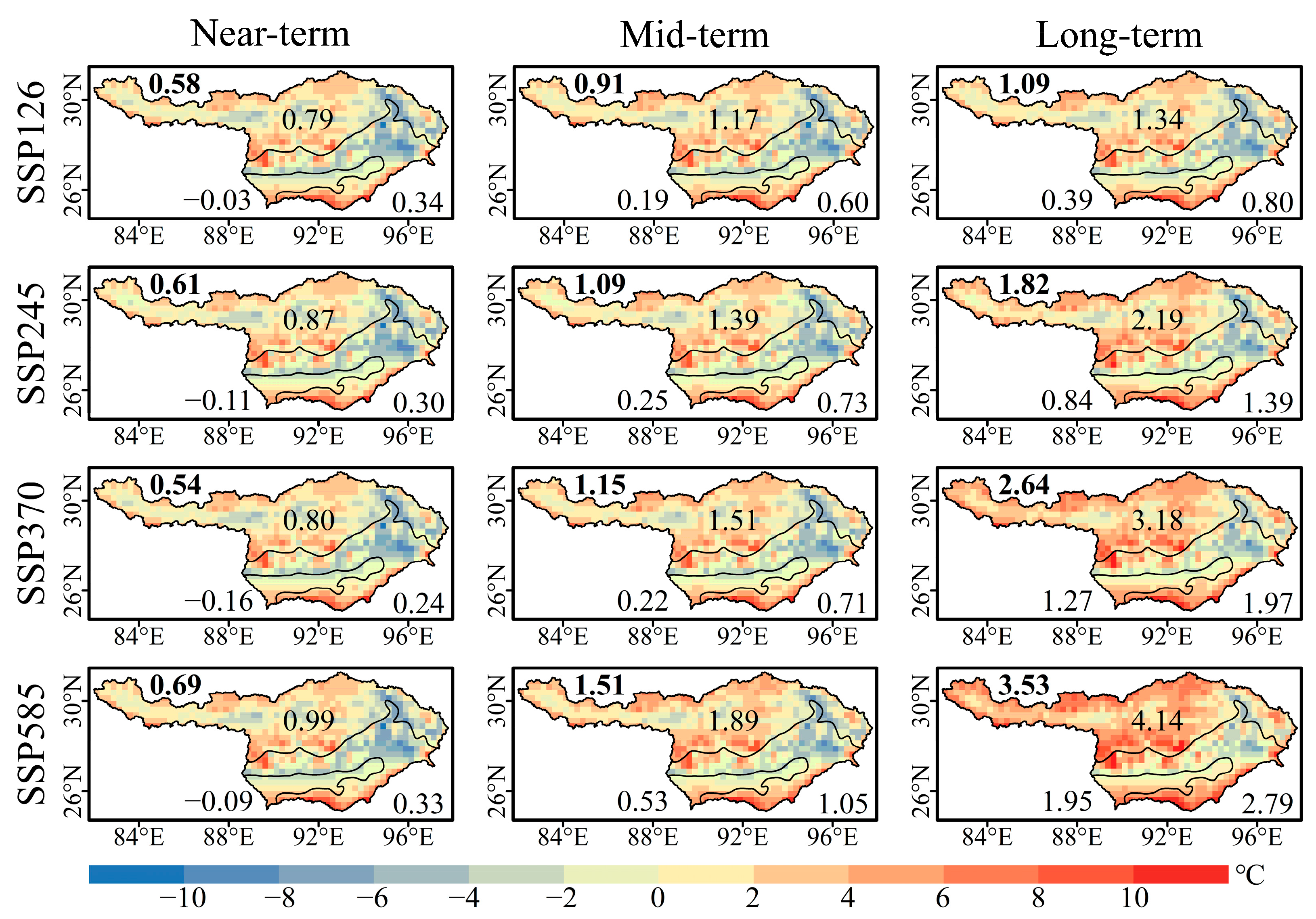
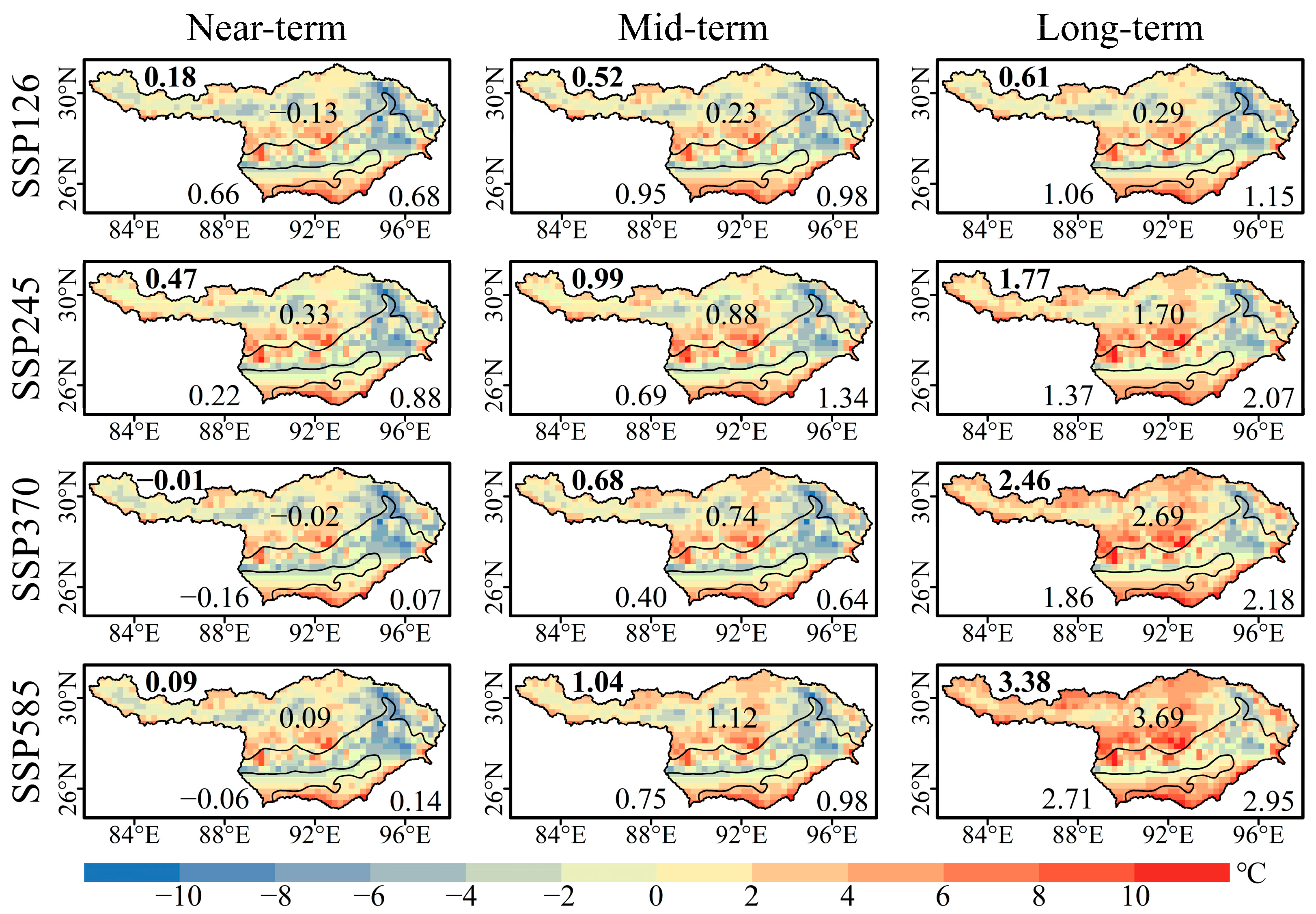
Figure 6 and Figure 7 present the predicted spatial patterns of annual surface Tmax and Tmin from the BMA over the YBRB across the near- (2021–2040), mid- (2041–2060), and long-term periods (2081–2100) relative to the reference period (1995–2014) under SSP126, SSP245, SSP370, and SSP585, respectively. By sub-region, the TP displayed the most significant future increase in Tmax, followed by the HB and the FP. Comparatively, there was no significant difference observed for Tmin by sub-region. In addition, with the increase in radiative forcing, the change amplitudes of Tmax and Tmin over the YBRB showed an overall increasing trend, especially among scenarios over the mid- and long-terms. According to the Sixth Assessment Report of the IPCC and the results of this study [1], when compared with the historical reference period (1995–2014), the global temperatures (Tmax; Tmin over the YBRB) in the near term will increase by 0.7, 0.7, 0.7, and 0.8 °C (0.58, 0.61, 0.54, and 0.69 °C; 0.18, 0.47, −0.01, and 0.09 °C) under scenarios SSP126, SSP245, SSP370, and SSP585, respectively; whereas those across the mid- and long-terms will increase by 1.0, 1.3, 1.4, and 1.7 °C (0.91, 1.09, 1.15, and 1.51 °C; 0.52, 0.99, 0.68, and 1.04 °C) and 1.2, 2.0, 3.1, and 4.0 °C (1.09, 1.82, 2.64, and 3.53 °C; 0.61, 1.77, 2.46, and 3.38 °C), respectively.
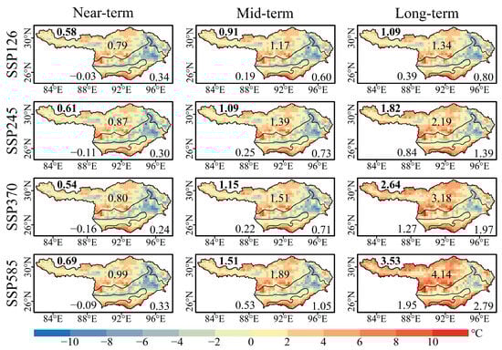
Figure 6.
Spatial patterns of annual surface Tmax from the BMA across the YBRB over the near- (2021–2040), mid- (2041–2060), and long-terms (2081–2100) relative to 1995–2014 under SSP126, SSP245, SSP370, and SSP585. Standard and bold numbers represent the average annual surface mean Tmax of the three sub-regions (°C) and basin, respectively.
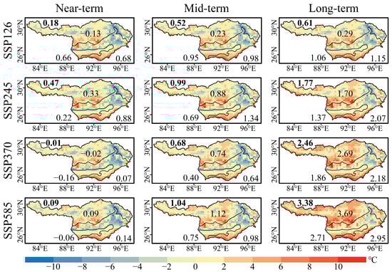
Figure 7.
Spatial patterns of annual surface Tmin from the BMA across the YBRB over the near- (2021–2040), mid- (2041–2060), and long-terms (2081–2100) relative to 1995–2014 under SSP126, SSP245, SSP370, and SSP585. Standard and bold numbers represent the average annual surface mean Tmin of the three sub-regions (°C) and basin, respectively.
Notably, the future increases in Tmax and Tmin over the YBRB both fell below the global averages; however, the increase (decrease) in Tmax (Tmin) over the TP was greater (lesser) than these averages, indicating that the importance of spatial differentiation over the YBRB in the future. Additionally, the increase in future Tmin over the YBRB was lower than that of Tmax, indicating a larger temperature difference in the future. The significant increase in Tmax is expected to intensify glacier and snow melting, leading to an escalated risk of water-related disasters such as glacial lake outburst floods and ice avalanches [55]. Conversely, the summer peak flows will increase, posing a greater flood threat to downstream areas [56,57]. From a water resources perspective, while the immediate effect of ice and snow melting may temporarily increase runoff, the long-term reduction in ice and snow water storage will ultimately lead to decreased runoff, thereby jeopardizing the food security of approximately 26 million people in downstream regions [58]. In summary, the temperature changes will exacerbate the transboundary water security risks in the YBRB.
3.4. Uncertainty in Future Temperature Projections
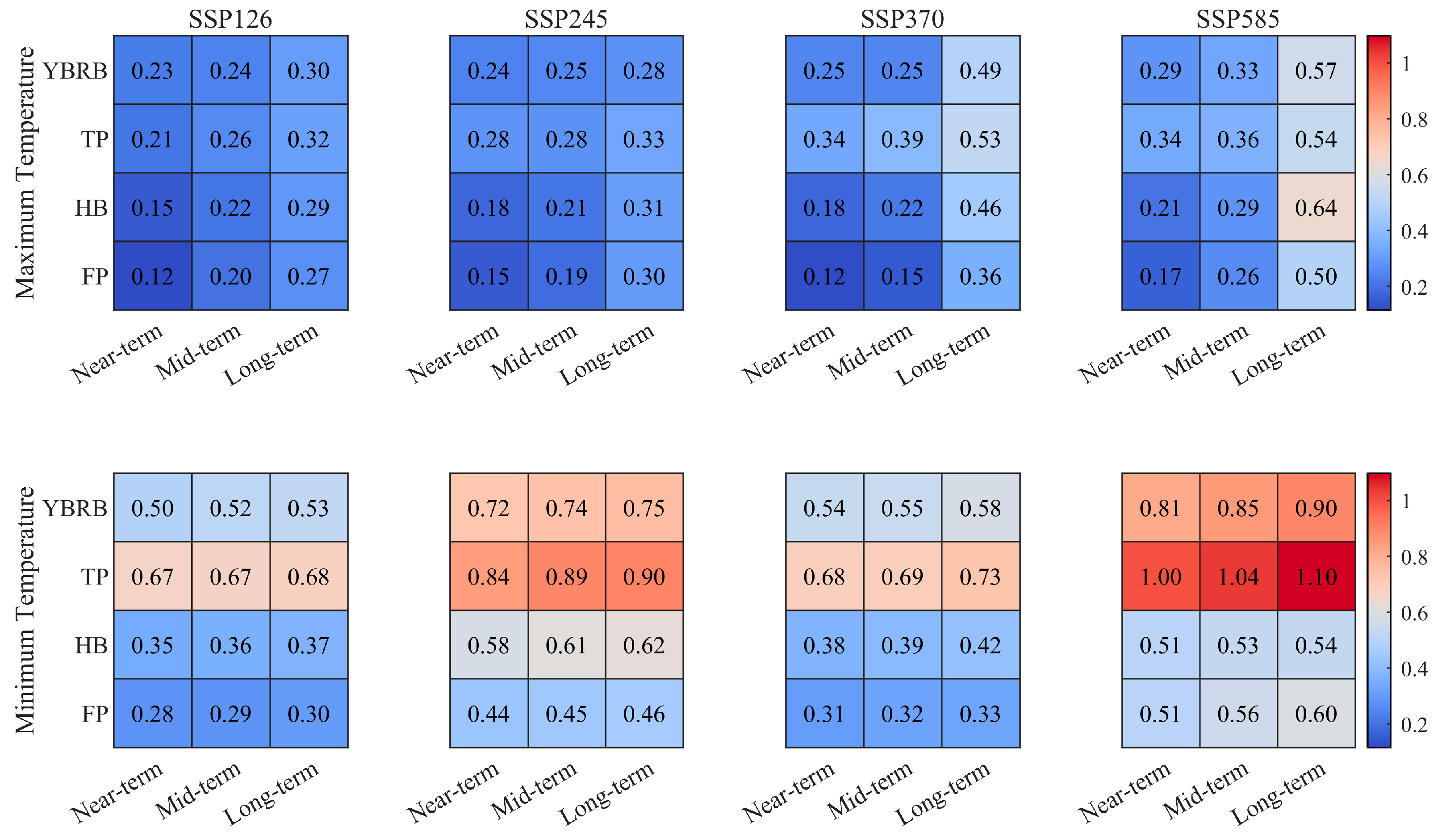
Uncertainty is inevitable during predictions of climate change [59,60], as future impacts on climate (whether man-made or natural) are inherently complex [61]. Accordingly, for projections to be applicable to future climate mitigation and strategic planning, it is necessary to quantify model uncertainty. To this end, model deviation can be used to assess the BMA climate projections [62], where the greater the deviation between the models (i.e., the larger the difference between them in simulating the Tmax and Tmin), the greater the uncertainty and lower the reliability of the predicted results. Figure 8 shows the uncertainty of the BMA-projected YBRB temperature changes over the near-, mid-, and long-term under the four future development scenarios. It was found that the uncertainty of the Tmax was smaller than that of the Tmin. Further, within the same region under the same scenario, the uncertainty of the two temperature variables increased with the forecast time. Across different regions, the TP displayed the largest uncertainty, followed by the HB and the FP. The strong uncertainty associated with the TP region may be related to the complex cryosphere environment. For example, albedo feedback is distorted owing to extensive snow cover over the plateau, potentially leading to large uncertainties in regional future climate projections [33].

Figure 8.
Annual surface Tmax and Tmin uncertainty (°C) over the YBRB and its three sub-regions over the near- (2021–2040), mid- (2041–2060), and long-terms (2081–2100) from the BMA under SSP126, SSP245, SSP370, and SSP585.
Additionally, uncertainty within the predicted results may also be related to model selection. Here, nine climate models were chosen for incorporation in BMA modeling, while intentionally excluding other CMIP6 models. Although this selection was made according to the frequency of use in existing studies (see Table S1 in Supporting Information), these assessments were based only on statistical results, and other models with potentially excellent performances across the study area may have been excluded. In future climate projections, further consideration should be given to using improved and more comprehensive climate model data to further reduce data uncertainty.
Nevertheless, the BMA multi-modal ensemble method produces decreased uncertainty compared with the traditional MME results and single models [29,30,31], as was confirmed in the present study (Section 3.1). While improving model algorithms and accuracies should be sought after, the remaining uncertainty must not deter those working on climate impact, mitigation, and adaptation from making critical decisions [63].
4. Conclusions
Taking the YBRB as a study area, the Tmax and Tmin performances over a historical period (2005–2014) were evaluated using nine CMIP6 climate models based on the BMA, and the aggregate average data fusion of the Tmax and Tmin under four future scenarios (SSP126, SSP245, SSP370, and SSP585) was performed according to the corresponding weight coefficients. On this basis, future changes in the Tmax and Tmin were estimated, and the following conclusions were drawn:
- (1)
- By comparing the performances of the Tmax and Tmin via the RMSE and ACC, the BMA-simulation effect on the Tmax and Tmin was deemed superior to that of the MME or individual models. Regional comparisons further revealed that the BMA could better simulate the Tmax and Tmin over the HB versus the TP or FP. By comparing the model weights, it was found that CanESM5 and ACCESS-ESM1-5 were the top performers for the Tmax and Tmin, respectively.
- (2)
- According to the BMA prediction results, the Tmax and Tmin over the YBRB during 2015–2100 fluctuated upwards under each of the four scenarios, with their respective warming rates increasing with scenario intensity. Under the most ideal sustainable development scenario (SSP126), the increase in the Tmax over the near-, mid-, and long-terms will reach 0.58, 0.91, and 1.09 °C across the YBRB; whereas the increases of the Tmin will reach 0.18, 0.52, and 0.61 °C, respectively. Under the high emissions scenario (SSP585), the increases in the Tmax (Tmin) over the near-, mid-, and long-terms are 0.69 (0.09), 1.51 (1.04), and 3.53 (3.38) °C, respectively. Although the overall future increases in the Tmax and Tmin are predicted to fall below global averages, the spatial differentiation of temperature in the upper and lower reaches of the basin will be more obvious.
- (3)
- The uncertainty of the future Tmax was smaller than that of the Tmin according to the BMA-derived results. In general, uncertainty increased with the prediction time, while spatially, the regions with the uncertainty were the TP > HB > FP.
In general, the BMA simulations outperformed traditional ensemble averages and individual models, which will lead to significant improvements for climatic projections over the YBRB. The inevitable and ongoing uncertainties should not affect our macro-cognition of the future temperature change characteristics across the YBRB. Further assessment to reduce the uncertainty of the estimated results is part of our future work.
Supplementary Materials
The following supporting information can be downloaded at: https://www.mdpi.com/article/10.3390/w15203595/s1, Table S1: Basic information and occurrence times of nine CMIP6 climate models; Text S1: Determine the optimal training period. References [64,65,66,67,68,69,70,71,72,73,74,75,76,77,78,79,80,81,82,83,84,85,86,87,88,89,90,91] are cited in the supplementary materials.
Author Contributions
Conceptualization, Z.X. and X.J.; The acquisition, analysis, or interpretation of data, Z.X., X.J., L.C., P.Q.; Methodology, Z.X. and X.J.; The analysis, or interpretation of data, Z.X. and X.J.; Writing—Original Draft Preparation, Z.X.; Writing—Review & Editing, Z.X. and X.J. All authors have read and agreed to the published version of the manuscript.
Funding
This research was funded by the National Natural Science Foundation of China (grant number: 42061005) and the Applied Basic Research Programs of Yunnan province (grant number: 202101AT070110). National College Student Innovation Training Program (grant number: 202110673060). College Student Innovation Training Program (grant number: 202004056).
Data Availability Statement
The relevant data are available from an online repository or repositories: For CMIP6 model dataset: https://esgf-node.llnl.gov/projects/cmip6/ (Accessed on 15 May 2022); for observation datasets: http://hydrology.princeton.edu/data/pgf/ (Accessed on 15 May 2022); for the Tmax and Tmin dataset after multi-model ensemble averaging: https://data.mendeley.com/datasets/s5z2sm9pfx/1 (Accessed on 2 October 2023).
Conflicts of Interest
The authors declare no conflict of interest.
References
- IPCC. Climate Change 2021: The Physical Science Basis: Working Group I Contribution to the Sixth Assessment Report of the Intergovernmental Panel on Climate Change; Masson-Delmotte, V.P., Zhaij, A., Pirani, S.L., Connors, C., Pean, S., Berger, N., Caud, Y., Chen, L., Goldfarb, M.l., Gomis, M., et al., Eds.; Cambridge University Press: Cambridge, UK; New York, NY, USA, 2021; p. 2391. ISBN 978-1-00-915789-6. [Google Scholar]
- Vousdoukas, M.I.; Mentaschi, L.; Voukouvalas, E.; Verlaan, M.; Jevrejeva, S.; Jackson, L.P.; Feyen, L. Global probabilistic projections of extreme sea levels show intensification of coastal flood hazard. Nat. Commun. 2018, 9, 2360. [Google Scholar] [CrossRef] [PubMed]
- Sun, Q.; Miao, C.; AghaKouchak, A.; Mallakpour, I.; Ji, D.; Duan, Q. Possible Increased Frequency of ENSO-Related Dry and Wet Conditions over Some Major Watersheds in a Warming Climate. Bull. Am. Meteorol. Soc. 2020, 101, E409–E426. [Google Scholar] [CrossRef]
- Kharin, V.V.; Flato, G.M.; Zhang, X.; Gillett, N.P.; Zwiers, F.; Anderson, K.J. Risks from Climate Extremes Change Differently from 1.5 °C to 2.0 °C Depending on Rarity. Earth’s Future 2018, 6, 704–715. [Google Scholar] [CrossRef]
- Lipczynska-Kochany, E. Effect of climate change on humic substances and associated impacts on the quality of surface water and groundwater: A review. Sci. Total Environ. 2018, 640–641, 1548–1565. [Google Scholar] [CrossRef]
- Zheng, H.; Miao, C.; Wu, J.; Lei, X.; Liao, W.; Li, H. Temporal and spatial variations in water discharge and sediment load on the Loess Plateau, China: A high-density study. Sci. Total Environ. 2019, 666, 875–886. [Google Scholar] [CrossRef] [PubMed]
- Jiang, T.; Su, B.; Huang, J.; Zhai, J.; Xia, J.; Tao, H.; Wang, Y.; Sun, H.; Luo, Y.; Zhang, L.; et al. Each 0. 5 °C of Warming Increases Annual Flood Losses in China by More than US$60 Billion. Bull. Am. Meteorol. Soc. 2020, 101, E1464–E1474. [Google Scholar] [CrossRef]
- Gou, J.; Miao, C.; Duan, Q.; Tang, Q.; Di, Z.; Liao, W.; Wu, J.; Zhou, R. Sensitivity Analysis-Based Automatic Parameter Calibration of the VIC Model for Streamflow Simulations Over China. Water Resour. Res. 2020, 56, e2019WR025968. [Google Scholar] [CrossRef]
- Schleussner, C.-F.; Donges, J.F.; Donner, R.V.; Schellnhuber, H.J. Armed-conflict risks enhanced by climate-related disasters in ethnically fractionalized countries. Proc. Natl. Acad. Sci. USA 2016, 113, 9216–9221. [Google Scholar] [CrossRef]
- Harari, M.; Ferrara, E.L. Conflict, Climate, and Cells: A Disaggregated Analysis. Rev. Econ. Stat. 2018, 100, 594–608. [Google Scholar] [CrossRef]
- Gao, J.; Yao, T.; Masson-Delmotte, V.; Steen-Larsen, H.C.; Wang, W. Collapsing glaciers threaten Asia’s water supplies. Nature 2019, 565, 19–21. [Google Scholar] [CrossRef]
- Kraaijenbrink, P.D.A.; Stigter, E.E.; Yao, T.; Immerzeel, W.W. Climate change decisive for Asia’s snow meltwater supply. Nat. Clim. Chang. 2021, 11, 591–597. [Google Scholar] [CrossRef]
- Yang, T.; Tao, Y.; Li, J.; Zhu, Q.; Su, L.; He, X.; Zhang, X. Multi-criterion model ensemble of CMIP5 surface air temperature over China. Theor. Appl. Climatol. 2018, 132, 1057–1072. [Google Scholar] [CrossRef]
- Zhu, H.; Jiang, Z.; Li, J.; Li, W.; Sun, C.; Li, L. Does CMIP6 Inspire More Confidence in Simulating Climate Extremes over China? Adv. Atmos. Sci. 2020, 37, 1119–1132. [Google Scholar] [CrossRef]
- Kim, Y.; Kim, W.; Ohn, I.; Kim, Y.-O. Leave-one-out Bayesian model averaging for probabilistic ensemble forecasting. Commun. Stat. Appl. Methods 2017, 24, 67–80. [Google Scholar] [CrossRef]
- Eyring, V.; Bony, S.; Meehl, G.A.; Senior, C.A.; Stevens, B.; Stouffer, R.J.; Taylor, K.E. Overview of the Coupled Model Intercomparison Project Phase 6 (CMIP6) experimental design and organization. Geosci. Model Dev. 2016, 9, 1937–1958. [Google Scholar] [CrossRef]
- IPCC. Climate Change 2001: The Scientific Basis. Contribution of Working Group I to the Third Assessment Report of the Intergovernmental Panel on Climate Change; Houghton, J.T., Ding, Y., Griggs, D.J., Noguer, M., van der Linden, P.J., Dai, X., Maskell, K., Johnson, C.A., Eds.; Cambridge University Press: Cambridge, UK; New York, NY, USA, 2001; p. 881. ISBN 0-521-80767-0. [Google Scholar]
- IPCC. Climate Change 2007: The Physical Science Basis. Contribution of Working Group I to the Fourth Assessment Report of the Intergovernmental Panel on Climate Change; Solomon, S.D., Qin, M., Manning, Z., Chen, M., Marquis, K.B., Averyt, M., Tignor, M., Eds.; Cambridge University Press: Cambridge, UK; New York, NY, USA, 2007; p. 996. ISBN 978-0-521-88009-1. [Google Scholar]
- IPCC. Climate Change 2013: The Physical Science Basis. Contribution of Working Group I to the Fifth Assessment Report of the Intergovernmental Panel on Climate Change; Stocker, T.F., Qin, D., Plattner, G.-K., Tignor, M., Allen, S.K., Boschung, J., Nauels, A., Xia, Y., Bex, V., Midgley, P.M., Eds.; Cambridge University Press: Cambridge, UK; New York, NY, USA, 2013; p. 1535. ISBN 978-1-107-05799-1. [Google Scholar]
- Feng, S.; Hu, Q.; Huang, W.; Ho, C.-H.; Li, R.; Tang, Z. Projected climate regime shift under future global warming from multi-model, multi-scenario CMIP5 simulations. Glob. Planet. Chang. 2014, 112, 41–52. [Google Scholar] [CrossRef]
- Zhao, T.; Chen, L.; Ma, Z. Simulation of historical and projected climate change in arid and semiarid areas by CMIP5 models. Chin. Sci. Bull. 2014, 59, 412–429. [Google Scholar] [CrossRef]
- Murphy, J.M.; Sexton, D.M.H.; Barnett, D.N.; Jones, G.S.; Webb, M.J.; Collins, M.; Stainforth, D.A. Quantification of modelling uncertainties in a large ensemble of climate change simulations. Nature 2004, 430, 768–772. [Google Scholar] [CrossRef]
- Schmittner, A.; Latif, M.; Schneider, B. Model projections of the North Atlantic thermohaline circulation for the 21st century assessed by observations. Geophys. Res. Lett. 2005, 32, L23710. [Google Scholar] [CrossRef]
- Tebaldi, C.; Smith, R.L.; Nychka, D.; Mearns, L.O. Quantifying Uncertainty in Projections of Regional Climate Change: A Bayesian Approach to the Analysis of Multimodel Ensembles. J. Clim. 2005, 18, 1524–1540. [Google Scholar] [CrossRef]
- Räisänen, J.; Ylhäisi, J.S. How Much Should Climate Model Output Be Smoothed in Space? J. Clim. 2011, 24, 867–880. [Google Scholar] [CrossRef]
- Wenzel, S.; Eyring, V.; Gerber, E.P.; Karpechko, A.Y. Constraining Future Summer Austral Jet Stream Positions in the CMIP5 Ensemble by Process-Oriented Multiple Diagnostic Regression. J. Clim. 2016, 29, 673–687. [Google Scholar] [CrossRef]
- Knutti, R.; Sedláček, J.; Sanderson, B.M.; Lorenz, R.; Fischer, E.M.; Eyring, V. A climate model projection weighting scheme accounting for performance and interdependence. Geophys. Res. Lett. 2017, 44, 1909–1918. [Google Scholar] [CrossRef]
- Sanderson, B.M.; Wehner, M.; Knutti, R. Skill and independence weighting for multi-model assessments. Geosci. Model Dev. 2017, 10, 2379–2395. [Google Scholar] [CrossRef]
- Raftery, A.E.; Gneiting, T.; Balabdaoui, F.; Polakowski, M. Using Bayesian Model Averaging to Calibrate Forecast Ensembles. Mon. Weather. Rev. 2005, 133, 1155–1174. [Google Scholar] [CrossRef]
- Sloughter, J.M.L.; Raftery, A.E.; Gneiting, T.; Fraley, C. Probabilistic Quantitative Precipitation Forecasting Using Bayesian Model Averaging. Mon. Weather. Rev. 2007, 135, 3209–3220. [Google Scholar] [CrossRef]
- Yang, T.; Wang, X.; Zhao, C.; Chen, X.; Yu, Z.; Shao, Q.; Xu, C.-Y.; Xia, J.; Wang, W. Changes of climate extremes in a typical arid zone: Observations and multimodel ensemble projections. J. Geophys. Res. Atmos. 2011, 116, D19106. [Google Scholar] [CrossRef]
- He, Y. Current and future transboundary water cooperation over the YarlungZangbo/Brahmaputra River basin: From an interdisciplinary perspective. Water Policy 2021, 23, 1107–1128. [Google Scholar] [CrossRef]
- Shi, Y.; Gao, X.; Zhang, D.; Giorgi, F. Climate change over the Yarlung Zangbo–Brahmaputra River Basin in the 21st century as simulated by a high resolution regional climate model. Quat. Int. 2011, 244, 159–168. [Google Scholar] [CrossRef]
- Immerzeel, W. Historical trends and future predictions of climate variability in the Brahmaputra basin. Int. J. Climatol. 2008, 28, 243–254. [Google Scholar] [CrossRef]
- Taylor, K.E.; Stouffer, R.J.; Meehl, G.A. An Overview of CMIP5 and the Experiment Design. Bull. Am. Meteorol. Soc. 2012, 93, 485–498. [Google Scholar] [CrossRef]
- Eyring, V.; Cox, P.M.; Flato, G.M.; Gleckler, P.J.; Abramowitz, G.; Caldwell, P.; Collins, W.D.; Gier, B.K.; Hall, A.D.; Hoffman, F.M.; et al. Taking climate model evaluation to the next level. Nat. Clim. Chang. 2019, 9, 102–110. [Google Scholar] [CrossRef]
- Masood, M.; Yeh, P.J.-F.; Hanasaki, N.; Takeuchi, K. Model study of the impacts of future climate change on the hydrology of Ganges-Brahmaputra-Meghna basin. Hydrol. Earth Syst. Sci. 2015, 19, 747–770. [Google Scholar] [CrossRef]
- Xu, R.; Hu, H.; Tian, F.; Li, C.; Khan, M.Y.A. Projected climate change impacts on future streamflow of the Yarlung Tsangpo-Brahmaputra River. Glob. Planet. Chang. 2019, 175, 144–159. [Google Scholar] [CrossRef]
- Gain, A.K.; Immerzeel, W.W.; Sperna Weiland, F.C.; Bierkens, M.F.P. Impact of climate change on the stream flow of the lower Brahmaputra: Trends in high and low flows based on discharge-weighted ensemble modelling. Hydrol. Earth Syst. Sci. 2011, 15, 1537–1545. [Google Scholar] [CrossRef]
- Jiang, W.; Ji, X.; Li, Y.; Luo, X.; Yang, L.; Ming, W.; Liu, C.; Yan, S.; Yang, C.; Sun, C. Modified flood potential index (MFPI) for flood monitoring in terrestrial water storage depletion basin using GRACE estimates. J. Hydrol. 2023, 616, 128765. [Google Scholar] [CrossRef]
- Pervez, M.S.; Henebry, G.M. Assessing the impacts of climate and land use and land cover change on the freshwater availability in the Brahmaputra River basin. J. Hydrol. Reg. Stud. 2015, 3, 285–311. [Google Scholar] [CrossRef]
- Beck, H.E.; Zimmermann, N.E.; McVicar, T.R.; Vergopolan, N.; Berg, A.; Wood, E.F. Present and future Köppen-Geiger climate classification maps at 1-km resolution. Sci. Data 2018, 5, 180214. [Google Scholar] [CrossRef] [PubMed]
- Guo, R.-Y.; Ji, X.; Liu, C.-Y.; Liu, C.; Jiang, W.; Yang, L.-Y. Spatiotemporal variation of snow cover and its relationship with temperature and precipitation in the Yarlung Tsangpo-Brahmaputra River Basin. J. Mt. Sci. 2022, 19, 1901–1918. [Google Scholar] [CrossRef]
- O’Neill, B.C.; Tebaldi, C.; van Vuuren, D.P.; Eyring, V.; Friedlingstein, P.; Hurtt, G.; Knutti, R.; Kriegler, E.; Lamarque, J.-F.; Lowe, J.; et al. The Scenario Model Intercomparison Project (ScenarioMIP) for CMIP6. Geosci. Model Dev. 2016, 9, 3461–3482. [Google Scholar] [CrossRef]
- Allabakash, S.; Lim, S. Anthropogenic influence of temperature changes across East Asia using CMIP6 simulations. Sci. Rep. 2022, 12, 11896. [Google Scholar] [CrossRef]
- Xie, A.; Zhu, J.; Kang, S.; Qin, X.; Xu, B.; Wang, Y. Polar amplification comparison among Earth’s three poles under different socioeconomic scenarios from CMIP6 surface air temperature. Sci. Rep. 2022, 12, 16548. [Google Scholar] [CrossRef] [PubMed]
- Ji, X.; Li, Y.; Luo, X.; He, D.; Guo, R.; Wang, J.; Bai, Y.; Yue, C.; Liu, C. Evaluation of bias correction methods for APHRODITE data to improve hydrologic simulation in a large Himalayan basin. Atmos. Res. 2020, 242, 104964. [Google Scholar] [CrossRef]
- Glahn, H.R.; Lowry, D.A. The Use of Model Output Statistics (MOS) in Objective Weather Forecasting. J. Appl. Meteorol. Climatol. 1972, 11, 1203–1211. [Google Scholar] [CrossRef]
- Carter, G.M.; Dallavalle, J.P.; Glahn, H.R. Statistical Forecasts Based on the National Meteorological Center’s Numerical Weather Prediction System. Weather Forecast. 1989, 4, 401–412. [Google Scholar] [CrossRef]
- Fisher, R.A. On the Mathematical Foundations of Theoretical Statistics. In Breakthroughs in Statistics: Foundations and Basic Theory; Kotz, S., Johnson, N.L., Eds.; Springer: New York, NY, USA, 1992; pp. 309–368. [Google Scholar]
- Mclachlan, G.J.; Krishnan, T. The EM Algorithm and Extensions; John Wiley & Sons, Ltd: Hoboken, NJ, USA, 2008. [Google Scholar]
- Pennell, C.; Reichler, T. On the Effective Number of Climate Models. J. Clim. 2011, 24, 2358–2367. [Google Scholar] [CrossRef]
- Lun, Y.; Liu, L.; Cheng, L.; Li, X.; Li, H.; Xu, Z. Assessment of GCMs simulation performance for precipitation and temperature from CMIP5 to CMIP6 over the Tibetan Plateau. Int. J. Climatol. 2021, 41, 3994–4018. [Google Scholar] [CrossRef]
- Zhu, Y.-Y.; Yang, S. Evaluation of CMIP6 for historical temperature and precipitation over the Tibetan Plateau and its comparison with CMIP5. Adv. Clim. Chang. Res. 2020, 11, 239–251. [Google Scholar] [CrossRef]
- Veh, G.; Korup, O.; Walz, A. Hazard from Himalayan glacier lake outburst floods. Proc. Natl. Acad. Sci. USA 2019, 117, 907–912. [Google Scholar] [CrossRef]
- Islam, A.K.M.S.; Paul, S.; Mohammed, K.; Billah, M.; Fahad, M.G.R.; Hasan, M.A.; Islam, G.M.T.; Bala, S.K. Hydrological response to climate change of the Brahmaputra basin using CMIP5 general circulation model ensemble. J. Water Clim. Chang. 2018, 9, 434–448. [Google Scholar] [CrossRef]
- Uhe, P.F.; Mitchell, D.M.; Bates, P.D.; Sampson, C.C.; Smith, A.M.; Islam, A.S. Enhanced flood risk with 1.5 °C global warming in the Ganges–Brahmaputra–Meghna basin. Environ. Res. Lett. 2019, 14, 074031. [Google Scholar] [CrossRef]
- Immerzeel, W.W.; van Beek, L.P.H.; Bierkens, M.F.P. Climate Change Will Affect the Asian Water Towers. Science 2010, 328, 1382–1385. [Google Scholar] [CrossRef]
- Allen, M.R.; Stott, P.A.; Mitchell, J.F.B.; Schnur, R.; Delworth, T.L. Quantifying the uncertainty in forecasts of anthropogenic climate change. Nature 2000, 407, 617–620. [Google Scholar] [CrossRef] [PubMed]
- Stott, P.A.; Kettleborough, J.A. Origins and estimates of uncertainty in predictions of twenty-first century temperature rise. Nature 2002, 416, 723–726. [Google Scholar] [CrossRef] [PubMed]
- Allen, M.; Raper, S.; Mitchell, J. Uncertainty in the IPCC’s Third Assessment Report. Science 2001, 293, 430–433. [Google Scholar] [CrossRef] [PubMed]
- Zhou, T.; Yu, R. Twentieth-Century Surface Air Temperature over China and the Globe Simulated by Coupled Climate Models. J. Clim. 2006, 19, 5843–5858. [Google Scholar] [CrossRef]
- Dessai, S.; Hulme, M.; Lempert, R.; Pielke Jr., R. Do We Need Better Predictions to Adapt to a Changing Climate? Eos Trans. Am. Geophys. Union 2009, 90, 111–112. [Google Scholar] [CrossRef]
- Chen, H.; Sun, J.; Lin, W.; Xu, H. Comparison of CMIP6 and CMIP5 models in simulating climate extremes. Sci. Bull. 2020, 65, 1415–1418. [Google Scholar] [CrossRef]
- Xin, X.; Wu, T.; Zhang, J.; Yao, J.; Fang, Y. Comparison of CMIP6 and CMIP5 simulations of precipitation in China and the East Asian summer monsoon. International. Int. J. Clim. 2020, 40, 6423–6440. [Google Scholar] [CrossRef]
- Zamani, Y.; Hashemi Monfared, S.A.; Azhdari moghaddam, M.; Hamidianpour, M. A comparison of CMIP6 and CMIP5 projections for precipitation to observational data: The case of Northeastern Iran. Theor. Appl. Climatol. 2020, 142, 1613–1623. [Google Scholar] [CrossRef]
- Almazroui, M.; Saeed, S.; Saeed, F.; Islam, M.N.; Ismail, M. Projections of Precipitation and Temperature over the South Asian Countries in CMIP6. Earth Syst. Environ. 2020, 4, 297–320. [Google Scholar] [CrossRef]
- Rivera, J.A.; Arnould, G. Evaluation of the ability of CMIP6 models to simulate precipitation over Southwestern South America: Climatic features and long-term trends (1901–2014). Atmos. Res. 2020, 241, 104953. [Google Scholar] [CrossRef]
- Jiang, J.; Zhou, T.; Chen, X.; Zhang, L. Future changes in precipitation over Central Asia based on CMIP6 projections. Environ. Res. Lett. 2020, 15, 054009. [Google Scholar] [CrossRef]
- Jiang, D.; Hu, D.; Tian, Z.; Lang, X. Differences between CMIP6 and CMIP5 Models in Simulating Climate over China and the East Asian Monsoon. Adv. Atmospheric Sci. 2020, 37, 1102–1118. [Google Scholar] [CrossRef]
- Qian, H.; Zhang, R. Future changes in wind energy resource over the Northwest Passage based on the CMIP6 climate projections. Int. J. Energy Res. 2021, 45, 920–937. [Google Scholar] [CrossRef]
- Wei, T.; Yan, Q.; Qi, W.; Ding, M.; Wang, C. Projections of Arctic sea ice conditions and shipping routes in the twenty-first century using CMIP6 forcing scenarios. Environ. Res. Lett. 2020, 15, 104079. [Google Scholar] [CrossRef]
- Burke, E.J.; Zhang, Y.; Krinner, G. Evaluating permafrost physics in the Coupled Model Intercomparison Project 6 (CMIP6) models and their sensitivity to climate change. Cryosphere 2020, 14, 3155–3174. [Google Scholar] [CrossRef]
- Akinsanola, A.A.; Kooperman, G.J.; Reed, K.A.; Pendergrass, A.G.; Hannah, W.M. Projected changes in seasonal precipitation extremes over the United States in CMIP6 simulations. Environ. Res. Lett. 2020, 15, 104078. [Google Scholar] [CrossRef]
- Cook, B.I.; Mankin, J.S.; Marvel, K.; Williams, A.P.; Smerdon, J.E.; Anchukaitis, K.J. Twenty-First Century Drought Projections in the CMIP6 Forcing Scenarios. Earth’s Futur. 2020, 8, e2019EF001461. [Google Scholar] [CrossRef]
- LI, J.; SU, J. Comparison of Indian Ocean warming simulated by CMIP5 and CMIP6 models. Atmospheric Ocean. Sci. Lett. 2020, 13, 604–611. [Google Scholar] [CrossRef]
- Guo, H.; Bao, A.; Chen, T.; Zheng, G.; Wang, Y.; Jiang, L.; De Maeyer, P. Assessment of CMIP6 in simulating precipitation over arid Central Asia. Atmospheric Res. 2021, 252, 105451. [Google Scholar] [CrossRef]
- Wild, M. The global energy balance as represented in CMIP6 climate models. Clim. Dyn. 2020, 55, 553–577. [Google Scholar] [CrossRef] [PubMed]
- Tokarska, K.B.; Stolpe, M.B.; Sippel, S.; Fischer, E.M.; Smith, C.J.; Lehner, F.; Knutti, R. Past warming trend constrains future warming in CMIP6 models. Sci. Adv. 2020, 6, eaaz9549. [Google Scholar] [CrossRef]
- Moseid, K.O.; Schulz, M.; Storelvmo, T.; Julsrud, I.R.; Olivie, D.; Nabat, P.; Wild, M.; Cole, J.N.S.; Takemura, T.; Oshima, N.; et al. Bias in CMIP6 models as compared to observed regional dimming and brightening. Atmospheric Meas. Tech. 2020, 20, 16023–16040. [Google Scholar] [CrossRef]
- Schlund, M.; Lauer, A.; Gentine, P.; Sherwood, S.C.; Eyring, V. Emergent constraints on equilibrium climate sensitivity in CMIP5: Do they hold for CMIP6? Earth Syst. Dyn. 2020, 11, 1233–1258. [Google Scholar] [CrossRef]
- Zhai, J.; Mondal, S.K.; Fischer, T.; Wang, Y.; Su, B.; Huang, J.; Tao, H.; Wang, G.; Ullah, W.; Uddin, M.J. Future drought characteristics through a multi-model ensemble from CMIP6 over South Asia. Atmospheric Res. 2020, 246, 105111. [Google Scholar] [CrossRef]
- Nooni, I.K.; Ogou, F.K.; Chaibou, A.A.S.; Nakoty, F.M.; Gnitou, G.T.; Lu, J. Evaluating CMIP6 Historical Mean Precipitation over Africa and the Arabian Peninsula against Satellite-Based Observation. Atmosphere 2023, 14, 607. [Google Scholar] [CrossRef]
- Zhang, C.; Qi, W.; Dong, J.; Deng, Y. How the CMIP6 climate models project the historical terrestrial GPP in China. Int. J. Clim. 2022, 42, 9449–9461. [Google Scholar] [CrossRef]
- Agyekum, J.; Annor, T.; Quansah, E.; Lamptey, B.; Okafor, G. Extreme precipitation indices over the Volta Basin: CMIP6 model evaluation. Sci. Afr. 2022, 16, e01181. [Google Scholar] [CrossRef]
- Makula, E.K.; Zhou, B. Coupled Model Intercomparison Project phase 6 evaluation and projection of East African precipitation. Int. J. Clim. 2022, 42, 2398–2412. [Google Scholar] [CrossRef]
- Deepthi, B.; Sivakumar, B. Shortest path length for evaluating general circulation models for rainfall simulation. Clim. Dyn. 2023, 61, 3009–3028. [Google Scholar] [CrossRef]
- Lin, X.; Massonnet, F.; Fichefet, T.; Vancoppenolle, M. Impact of atmospheric forcing uncertainties on Arctic and Antarctic sea ice simulations in CMIP6 OMIP models. Cryosphere 2023, 17, 1935–1965. [Google Scholar] [CrossRef]
- Allende, S.; Fichefet, T.; Goosse, H.; Treguier, A.M. On the ability of OMIP models to simulate the ocean mixed layer depth and its seasonal cycle in the Arctic Ocean. Ocean Model. 2023, 184, 102226. [Google Scholar] [CrossRef]
- Shiru, M.S.; Chung, E.-S. Performance evaluation of CMIP6 global climate models for selecting models for climate projection over Nigeria. Theor. Appl. Clim. 2021, 146, 599–615. [Google Scholar] [CrossRef]
- Deepthi, B.; Sivakumar, B. General circulation models for rainfall simulations: Performance assessment using complex networks. Atmospheric Res. 2022, 278, 106333. [Google Scholar] [CrossRef]
Disclaimer/Publisher’s Note: The statements, opinions and data contained in all publications are solely those of the individual author(s) and contributor(s) and not of MDPI and/or the editor(s). MDPI and/or the editor(s) disclaim responsibility for any injury to people or property resulting from any ideas, methods, instructions or products referred to in the content. |
© 2023 by the authors. Licensee MDPI, Basel, Switzerland. This article is an open access article distributed under the terms and conditions of the Creative Commons Attribution (CC BY) license (https://creativecommons.org/licenses/by/4.0/).