
Spatial Effects of NAO on Temperature and Precipitation Anomalies in Italy
 , ,
, ,  ,
,
Abstract
:1. Introduction
1.1. Aim of the Study and State of the Art
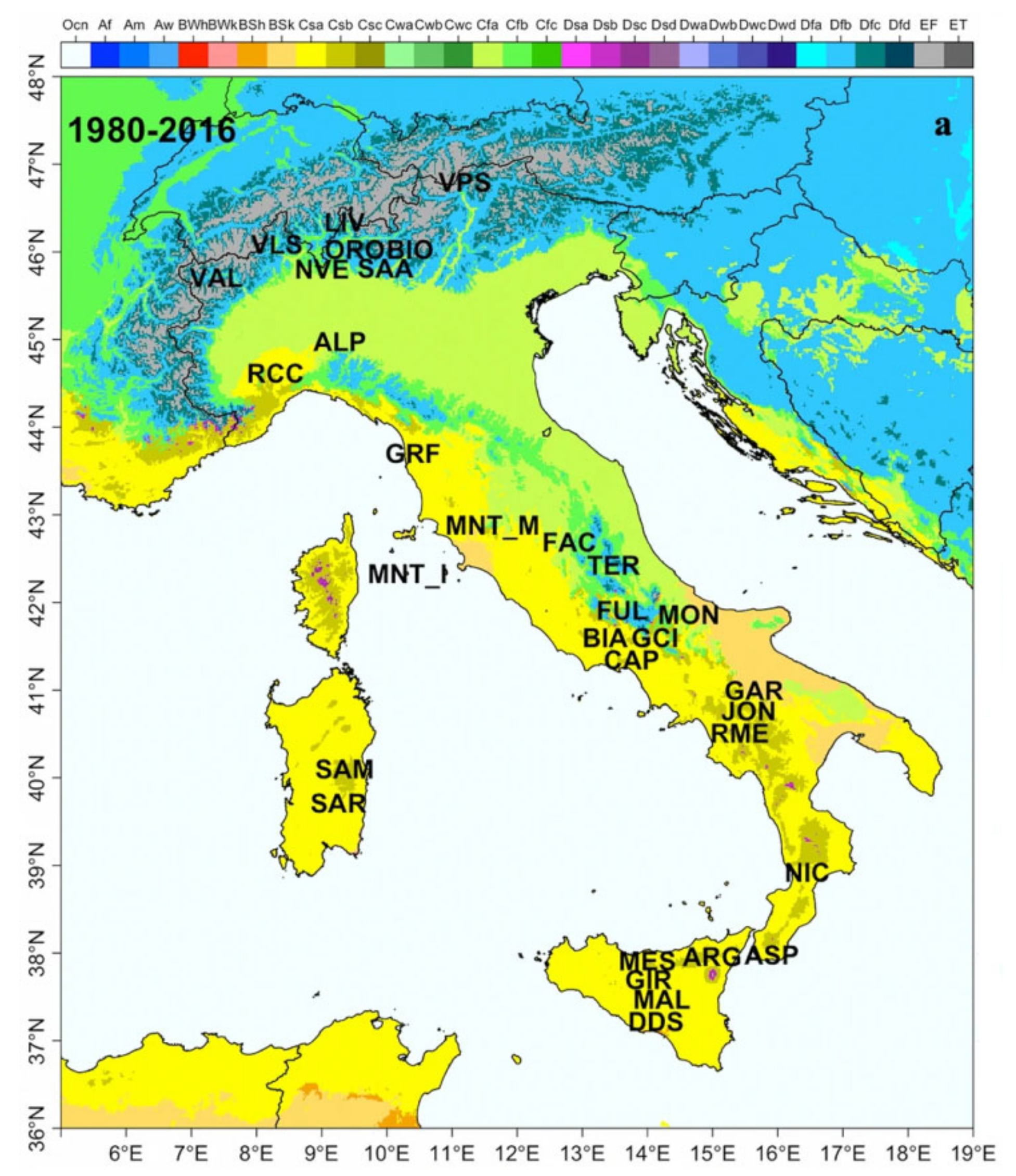
1.2. Study Area
2. Materials and Methods
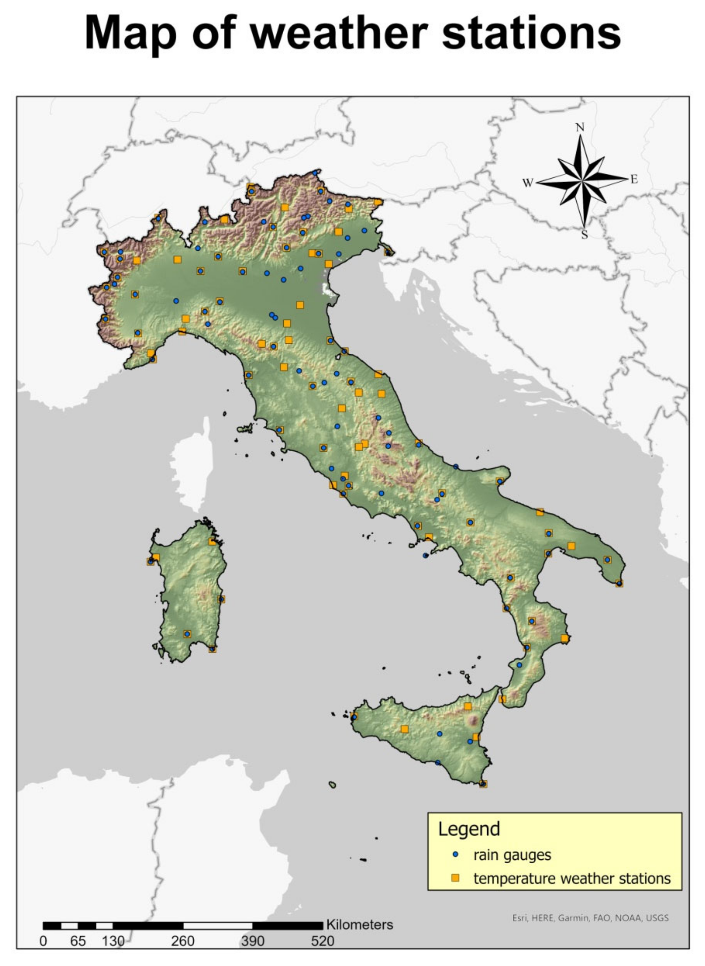
2.1. Weather Stations
2.2. NAO Index
2.3. Statistical Analysis
- = dependent variable;
- = independent variable;
- = intercept value;
- = slope value;
- = error term, consists of omitted factors, other than variable , that influence , the regression error (error term) also includes the error in the measurement of .
2.4. Clusters and Outliers Analysis
- = value of the variable z at location i;
- = average value of z;
- = value of variable z in all other locations other than i;
- = variance of z;
- = weight, inverse distance among locations i and j.
3. Results
3.1. Correlation Analysis between NAO Index and Climate Variables
3.2. Regression Analysis between NAO Index and Climate Variables
3.3. Analysis of Clusters and Outliers
4. Discussion
4.1. Interpretations and Implications
4.2. Research Limitations
5. Conclusions
- The correlation between the NAO index and temperature or precipitation anomalies was mapped for the entire Italian territory;
- A linear regression was obtained with the relevant coefficients of determination between the NAO index and temperature or precipitation anomalies;
- The presence of clusters and outliers in the study area was assessed.
Author Contributions
Funding
Data Availability Statement
Conflicts of Interest
References
- Wanner, H.; Brönnimann, S.; Casty, C.; Gyalistras, D.; Luterbacher, J.; Schmutz, C.; Stephenson, D.B.; Xoplaki, E. North Atlantic Oscillation–concepts and studies. Surv. Geophys. 2001, 22, 321–381. [Google Scholar] [CrossRef]
- Hurrell, J.W.; Kushnir, Y.; Ottersen, G.; Visbeck, M. An overview of the North Atlantic oscillation. Geophys. Monogr.-Am. Geophys. Union 2003, 134, 1–36. [Google Scholar]
- Wrzesiński, D.; Paluszkiewicz, R. Spatial differences in the impact of the North Atlantic Oscillation on the flow of rivers in Europe. Hydrol. Res. 2011, 42, 30–39. [Google Scholar] [CrossRef]
- Massei, N.; Laignel, B.; Deloffre, J.; Mesquita, J.; Motelay, A.; Lafite, R.; Durand, A. Long-term hydrological changes of the Seine River flow (France) and their relation to the North Atlantic Oscillation over the period 1950–2008. Int. J. Climatol. 2010, 30, 2146–2154. [Google Scholar] [CrossRef]
- Rîmbu, N.; Boroneanţ, C.; Buţă, C.; Dima, M. Decadal variability of the Danube river flow in the lower basin and its relation with the North Atlantic Oscillation. Int. J. Climatol. 2002, 22, 1169–1179. [Google Scholar] [CrossRef]
- Trigo, R.M. The impacts of the NAO on hydrological resources of the Western Mediterranean. In Hydrological, Socioeconomic and Ecological Impacts of the North Atlantic Oscillation in the Mediterranean Region; Springer: Dordrecht, The Netherlands, 2011; pp. 41–56. [Google Scholar] [CrossRef]
- Zanchettin, D.; Rubino, A.; Traverso, P.; Tomasino, M. Impact of variations in solar activity on hydrological decadal patterns in northern Italy. J. Geophys. Res. Atmos. 2008, 113, 1–12. [Google Scholar] [CrossRef]
- Zanchettin, D.; Toniazzo, T.; Taricco, C.; Rubinetti, S.; Rubino, A.; Tartaglione, N. Atlantic origin of asynchronous European interdecadal hydroclimate variability. Sci. Rep. 2019, 9, 10998. [Google Scholar] [CrossRef]
- Gordo, O.; Barriocanal, C.; Robson, D. Ecological impacts of the North Atlantic Oscillation (NAO) in Mediterranean ecosystems. In Hydrological, Socioeconomic and Ecological Impacts of the North Atlantic Oscillation in the Mediterranean Region; Springer: Berlin/Heidelberg, Germany, 2011; pp. 153–170. [Google Scholar] [CrossRef]
- Camarero, J.J. Direct and indirect effects of the North Atlantic Oscillation on tree growth and forest decline in northeastern Spain. In Hydrological, Socioeconomic and Ecological Impacts of the North Atlantic Oscillation in the Mediterranean Region; Springer: Dordrecht, The Netherlands, 2011; pp. 129–152. [Google Scholar] [CrossRef]
- Lindholm, M.; Eggertsson, Ó.; Lovelius, N.; Raspopov, O.; Shumilov, O.; Laanelaid, A. Growth indices of north European Scots pine record the seasonal North Atlantic Oscillation. Boreal Environ. Res. 2001, 6, 275–284. [Google Scholar]
- Haest, B.; Hüppop, O.; Bairlein, F. Challenging a 15-year-old claim: The North Atlantic Oscillation index as a predictor of spring migration phenology of birds. Glob. Change Biol. 2018, 24, 1523–1537. [Google Scholar] [CrossRef]
- Piontkovski, S.A.; O’brien, T.D.; Umani, S.F.; Krupa, E.G.; Stuge, T.S.; Balymbetov, K.S.; Grishaeva, O.V.; Kasymov, A.G. Zooplankton and the North Atlantic Oscillation: A basin-scale analysis. J. Plankton Res. 2006, 28, 1039–1046. [Google Scholar] [CrossRef]
- Lynam, C.P.; Hay, S.J.; Brierley, A.S. Interannual variability in abundance of North Sea jellyfish and links to the North Atlantic Oscillation. Limnol. Oceanogr. 2004, 49, 637–643. [Google Scholar] [CrossRef]
- Tsimplis, M.N.; Calafat, F.M.; Marcos, M.; Jordá, G.; Gomis, D.; Fenoglio-Marc, L.; Struglia, M.V.; Josey, S.A.; Chambers, D.P. The effect of the NAO on sea level and on mass changes in the Mediterranean Sea. J. Geophys. Res. Oceans 2013, 118, 944–952. [Google Scholar] [CrossRef]
- Qu, B.; Gabric, A.J.; Zhu, J.N.; Lin, D.R.; Qian, F.; Zhao, M. Correlation between sea surface temperature and wind speed in Greenland Sea and their relationships with NAO variability. Water Sci. Eng. 2012, 5, 304–315. [Google Scholar] [CrossRef]
- Seierstad, I.A.; Bader, J. Impact of a projected future Arctic sea ice reduction on extratropical storminess and the NAO. Clim. Dyn. 2009, 33, 937–943. [Google Scholar] [CrossRef]
- Wang, X.L.; Zwiers, F.W.; Swail, V.R.; Feng, Y. Trends and variability of storminess in the Northeast Atlantic region, 1874–2007. Clim. Dyn. 2009, 33, 1179–1195. [Google Scholar] [CrossRef]
- Choi, J.W.; Cha, Y. Possible relationship between NAO and tropical cyclone genesis frequency in the western North Pacific. Dyn. Atmos. 2017, 77, 64–73. [Google Scholar] [CrossRef]
- Krichak, S.O.; Breitgand, J.S.; Gualdi, S.; Feldstein, S.B. Teleconnection–extreme precipitation relationships over the Mediterranean region. Theor. Appl. Climatol. 2014, 117, 679–692. [Google Scholar] [CrossRef]
- Qian, B.; Corte-Real, J.; Xu, H. Is the North Atlantic Oscillation the most important atmospheric pattern for precipitation in Europe? J. Geophys. Res. Atmos. 2000, 105, 11901–11910. [Google Scholar] [CrossRef]
- Castro-Díez, Y.; Pozo-Vázquez, D.; Rodrigo, F.S.; Esteban-Parra, M.J. NAO and winter temperature variability in southern Europe. Geophys. Res. Lett. 2002, 29, 1-1–1-4. [Google Scholar] [CrossRef]
- Raible, C.C.; Lehner, F.; González-Rouco, J.F.; Fernández-Donado, L. Changing correlation structures of the Northern Hemisphere atmospheric circulation from 1000 to 2100 AD. Clim. Past 2014, 10, 537–550. [Google Scholar] [CrossRef]
- Vicente-Serrano, S.M.; López-Moreno, J.I. Nonstationary influence of the North Atlantic Oscillation on European precipitation. J. Geophys. Res. Atmos. 2008, 113, D20120. [Google Scholar] [CrossRef]
- Pozo-Vázquez, D.; Esteban-Parra, M.J.; Rodrigo, F.S.; Castro-Díez, Y. A study of NAO variability and its possible non-linear influences on European surface temperature. Clim. Dyn. 2001, 17, 701–715. [Google Scholar] [CrossRef]
- López-Moreno, J.I.; Vicente-Serrano, S.M.; Morán-Tejeda, E.; Lorenzo-Lacruz, J.; Kenawy, A.; Beniston, M. Effects of the North Atlantic Oscillation (NAO) on combined temperature and precipitation winter modes in the Mediterranean mountains: Observed relationships and projections for the 21st century. Glob. Planet. Change 2011, 77, 62–76. [Google Scholar] [CrossRef]
- Cortellari, M.; Barbato, M.; Talenti, A.; Bionda, A.; Carta, A.; Ciampolini, R.; Ciani, E.; Crisà, A.; Frattini, S.; Lasagna, E.; et al. The climatic and genetic heritage of Italian goat breeds with genomic SNP data. Sci. Rep. 2021, 11, 10986. [Google Scholar] [CrossRef] [PubMed]
- Antonetti, G.; Gentilucci, M.; Aringoli, D.; Pambianchi, G. Analysis of landslide Susceptibility and Tree Felling Due to an Extreme Event at Mid-Latitudes: Case Study of Storm Vaia, Italy. Land 2022, 11, 1808. [Google Scholar] [CrossRef]
- Estévez, J.; Gavilán, P.; Giráldez, J.V. Guidelines on validation procedures for meteorological data from automatic weather stations. J. Hydrol. 2011, 402, 144–154. [Google Scholar] [CrossRef]
- Gentilucci, M.; Barbieri, M.; Burt, P.; D’Aprile, F. Preliminary data validation and reconstruction of temperature and precipitation in Central Italy. Geosciences 2018, 8, 202. [Google Scholar] [CrossRef]
- Wijngaard, J.B.; Klein Tank, A.M.G.; Können, G.P. Homogeneity of 20th century European daily temperature and precipitation series. Int. J. Climatol. J. R. Meteorol. Soc. 2003, 23, 679–692. [Google Scholar] [CrossRef]
- Peifer, H. About the EEA Reference Grid; European Environment Agency: Copenhagen, Denmark, 2011. [Google Scholar]
- Stenseth, N.C.; Ottersen, G.; Hurrell, J.W.; Mysterud, A.; Lima, M.; Chan, K.S.; Yoccoz, N.G.; Ådlandsvik, B. Studying climate effects on ecology through the use of climate indices: The North Atlantic Oscillation, El Nino Southern Oscillation and beyond. Proceedings of the Royal Society of London. Ser. B Biol. Sci. 2003, 270, 2087–2096. [Google Scholar] [CrossRef] [PubMed]
- Hannachi, A.; Woollings, T.; Turner, A. Atmospheric Low Frequency Variability: The Examples of the North Atlantic and the Indian Monsoon. In Climate Variability-Some Aspects, Challenges and Prospects; IntechOpen: London, UK, 2012. [Google Scholar]
- Osborn, T.J. Winter 2009/2010 temperatures and a record-breaking North Atlantic Oscillation index. Weather 2011, 66, 19–21. [Google Scholar] [CrossRef]
- Barnston, A.G.; Livezey, R.E. Classification, seasonality and persistence of low-frequency atmospheric circulation patterns. Mon. Weather. Rev. 1987, 115, 1083–1126. [Google Scholar] [CrossRef]
- Kistler, R.; Kalnay, E.; Collins, W.; Saha, S.; White, G.; Woollen, J.; Chelliah, M.; Ebisuzaki, W.; Kanamitsu, M.; Kousky, V.; et al. The NCEP–NCAR 50-year reanalysis: Monthly means CD-ROM and documentation. Bull. Am. Meteorol. Soc. 2001, 82, 247–268. Available online: https://www.jstor.org/stable/26215517 (accessed on 16 January 2023). [CrossRef]
- Ning, L.; Bradley, R.S. NAO and PNA influences on winter temperature and precipitation over the eastern United States in CMIP5 GCMs. Clim. Dyn. 2016, 46, 1257–1276. [Google Scholar] [CrossRef]
- Bromwich, D.H.; Chen, Q.S.; Li, Y.; Cullather, R.I. Precipitation over Greenland and its relation to the North Atlantic Oscillation. J. Geophys. Res. Atmos. 1999, 104, 22103–22115. [Google Scholar] [CrossRef]
- Gentilucci, M.; Pambianchi, G. Prediction of Snowmelt Days Using Binary Logistic Regression in the Umbria-Marche Apennines (Central Italy). Water 2022, 14, 1495. [Google Scholar] [CrossRef]
- Tsanis, I.; Tapoglou, E. Winter North Atlantic Oscillation impact on European precipitation and drought under climate change. Theor. Appl. Climatol. 2019, 135, 323–330. [Google Scholar] [CrossRef]
- Anselin, L. Local indicators of spatial association—LISA. Geogr. Anal. 1995, 27, 93–115. [Google Scholar] [CrossRef]
- Getis, A.; Ord, J.K. Local spatial statistics: An overview. In Spatial Analysis: Modelling in a GIS Environment; Longley, P., Batty, M., Eds.; GeoInformation International: Cambridge, UK, 1996; pp. 261–277. [Google Scholar]
- Levine, N. Crimestat IV: A Spatial Statistics Program for the Analysis of Crime Incident Locations, Version 4.0; Ned Levine & Associates: Houston, TX, USA, 2013. [Google Scholar]
- Zhang, C.; Luo, L.; Xu, W.; Ledwith, V. Use of local Moran’s I and GIS to identify pollution hotspots of Pb in urban soils of Galway, Ireland. Sci. Total Environ. 2008, 398, 212–221. [Google Scholar] [CrossRef] [PubMed]
- Toreti, A.; Desiato, F.; Fioravanti, G.; Perconti, W. Seasonal temperatures over Italy and their relationship with low-frequency atmospheric circulation patterns. Clim. Change 2010, 99, 211–227. [Google Scholar] [CrossRef]
- Brandimarte, L.; Di Baldassarre, G.; Bruni, G.; D’Odorico, P.; Montanari, A. Relation between the North-Atlantic Oscillation and hydroclimatic conditions in Mediterranean areas. Water Resour. Manag. 2011, 25, 1269–1279. [Google Scholar] [CrossRef]
- Boccolari, M.; Malmusi, S. Changes in temperature and precipitation extremes observed in Modena, Italy. Atmos. Res. 2013, 122, 16–31. [Google Scholar] [CrossRef]
- Vergni, L.; Di Lena, B.; Chiaudani, A. Statistical characterisation of winter precipitation in the Abruzzo region (Italy) in relation to the North Atlantic Oscillation (NAO). Atmos. Res. 2016, 178, 279–290. [Google Scholar] [CrossRef]
- Scorzini, A.R.; Leopardi, M. Precipitation and temperature trends over central Italy (Abruzzo Region): 1951–2012. Theor. Appl. Clim. 2019, 135, 959–977. [Google Scholar] [CrossRef]
- Delitala, A.M.; Cesari, D.; Chessa, P.A.; Ward, M.N. Precipitation over Sardinia (Italy) during the 1946–1993 rainy seasons and associated large-scale climate variations. Int. J. Climatol. J. R. Meteorol. Soc. 2000, 20, 519–541. [Google Scholar] [CrossRef]
- Bocchiola, D. Long term (1921–2011) hydrological regime of Alpine catchments in Northern Italy. Adv. Water Resour. 2014, 70, 51–64. [Google Scholar] [CrossRef]
- Bladé, I.; Liebmann, B.; Fortuny, D.; van Oldenborgh, G.J. Observed and simulated impacts of the summer NAO in Europe: Implications for projected drying in the Mediterranean region. Clim. Dyn. 2012, 39, 709–727. [Google Scholar] [CrossRef]
- Uvo, C.B. Analysis and regionalization of northern European winter precipitation based on its relationship with the North Atlantic Oscillation. Int. J. Climatol. J. R. Meteorol. Soc. 2003, 23, 1185–1194. [Google Scholar] [CrossRef]
- Gentilucci, M.; Catorci, A.; Panichella, T.; Moscatelli, S.; Hamed, Y.; Missaoui, R.; Pambianchi, G. Analysis of snow cover in the Sibillini Mountains in Central Italy. Climate 2023, 11, 72. [Google Scholar] [CrossRef]
- Gentilucci, M.; Barbieri, M.; Pambianchi, G. Reliability of the IMERG product through reference rain gauges in Central Italy. Atmos. Res. 2022, 278, 106340. [Google Scholar] [CrossRef]


| NORTH-WEST | WIN | SPR | SUM | AUT | JAN | FEB | MAR | APR | MAY | JUN | JUL | AUG | SEP | OCT | NOV | DEC |
|---|---|---|---|---|---|---|---|---|---|---|---|---|---|---|---|---|
| ALA DI STURA | 0.30 | 0.29 | 0.01 | 0.21 | 0.22 | 0.20 | 0.41 | 0.21 | 0.29 | 0.01 | 0.09 | −0.08 | 0.41 | 0.03 | 0.21 | 0.36 |
| ALBENGA | 0.31 | 0.26 | 0.15 | 0.19 | 0.11 | 0.27 | 0.44 | 0.18 | 0.20 | 0.07 | 0.11 | 0.27 | 0.29 | 0.01 | 0.24 | 0.45 |
| ALPE DEVERO | 0.31 | 0.22 | −0.02 | 0.23 | 0.26 | 0.15 | 0.32 | 0.14 | 0.16 | −0.09 | 0.04 | −0.03 | 0.35 | 0.02 | 0.30 | 0.50 |
| BERGAMO | 0.18 | 0.23 | 0.04 | 0.13 | 0.07 | 0.21 | 0.30 | 0.06 | 0.28 | 0.02 | −0.01 | 0.09 | 0.48 | −0.04 | 0.01 | 0.26 |
| BRESCIA/GHE | 0.14 | 0.23 | −0.11 | 0.11 | 0.03 | 0.21 | 0.34 | 0.12 | 0.29 | −0.04 | −0.15 | −0.11 | 0.33 | −0.03 | −0.03 | 0.16 |
| COGNE | 0.28 | 0.27 | 0.04 | 0.25 | 0.26 | 0.16 | 0.30 | 0.22 | 0.30 | 0.08 | 0.04 | 0.02 | 0.35 | −0.02 | 0.46 | 0.43 |
| DONNAS | 0.23 | 0.27 | 0.01 | 0.16 | 0.14 | 0.16 | 0.29 | 0.20 | 0.42 | 0.08 | −0.03 | −0.07 | 0.40 | −0.05 | 0.10 | 0.43 |
| FUNIVIA BERNINA-CHIESA VALMA | 0.25 | 0.23 | 0.07 | 0.22 | 0.15 | 0.12 | 0.34 | 0.18 | 0.28 | −0.01 | 0.09 | 0.12 | 0.30 | 0.01 | 0.42 | 0.43 |
| GENOVA/SESTRI | 0.37 | 0.23 | 0.09 | 0.15 | 0.31 | 0.27 | 0.34 | 0.02 | 0.27 | 0.01 | 0.12 | 0.11 | 0.39 | −0.12 | 0.14 | 0.55 |
| LA THUILE | 0.31 | 0.26 | 0.05 | 0.23 | 0.34 | 0.17 | 0.35 | 0.17 | 0.25 | 0.11 | 0.05 | 0.06 | 0.35 | −0.04 | 0.38 | 0.46 |
| MILANO/LINATE | 0.15 | 0.22 | 0.05 | 0.09 | 0.07 | 0.18 | 0.25 | 0.09 | 0.34 | 0.01 | 0.09 | 0.03 | 0.33 | −0.03 | −0.07 | 0.18 |
| MILANO/MALPENSA | 0.19 | 0.21 | −0.04 | 0.18 | 0.11 | 0.26 | 0.27 | 0.13 | 0.23 | −0.26 | 0.07 | 0.07 | 0.36 | 0.06 | 0.09 | 0.24 |
| MONDOVI | 0.31 | 0.19 | 0.05 | 0.18 | 0.32 | 0.14 | 0.37 | 0.01 | 0.13 | 0.08 | 0.11 | −0.03 | 0.36 | −0.05 | 0.20 | 0.52 |
| PASSO DEI GIOVI | 0.37 | 0.26 | 0.00 | 0.14 | 0.41 | 0.23 | 0.34 | 0.21 | 0.28 | −0.12 | 0.07 | 0.07 | 0.35 | −0.05 | 0.15 | 0.51 |
| PIETRASTRETTA | 0.33 | 0.24 | 0.03 | 0.21 | 0.39 | 0.17 | 0.40 | 0.06 | 0.30 | 0.03 | 0.09 | 0.00 | 0.31 | −0.01 | 0.29 | 0.47 |
| PONTECHIANALE | 0.35 | 0.27 | −0.02 | 0.17 | 0.43 | 0.23 | 0.36 | 0.13 | 0.36 | −0.07 | 0.03 | −0.03 | 0.30 | −0.09 | 0.28 | 0.52 |
| TORINO/BRIC | 0.31 | 0.17 | 0.05 | 0.25 | 0.35 | 0.20 | 0.38 | 0.06 | 0.13 | 0.06 | 0.05 | 0.12 | 0.46 | 0.00 | 0.29 | 0.46 |
| NORTH-EAST | WIN | SPR | SUM | AUT | JAN | FEB | MAR | APR | MAY | JUN | JUL | AUG | SEP | OCT | NOV | DEC |
| AVIANO | 0.18 | 0.25 | 0.07 | 0.12 | 0.06 | 0.26 | 0.36 | 0.16 | 0.28 | −0.05 | 0.08 | 0.16 | 0.35 | −0.01 | −0.05 | 0.24 |
| BOBBIO | 0.30 | 0.20 | −0.03 | 0.13 | 0.20 | 0.24 | 0.21 | 0.11 | 0.27 | −0.06 | −0.01 | −0.05 | 0.34 | −0.05 | 0.10 | 0.46 |
| BOLOGNA/BORGO | 0.22 | 0.27 | 0.00 | 0.04 | 0.11 | 0.27 | 0.31 | 0.06 | 0.44 | −0.02 | −0.03 | 0.02 | 0.22 | 0.00 | −0.14 | 0.27 |
| BOLZANO | 0.12 | 0.22 | −0.04 | 0.08 | −0.01 | 0.20 | 0.37 | 0.17 | 0.19 | −0.04 | −0.01 | −0.06 | 0.41 | −0.13 | −0.05 | 0.17 |
| BRUSTOLE’ VELO D’ASTICO | 0.19 | 0.26 | 0.01 | 0.16 | 0.05 | 0.25 | 0.35 | 0.14 | 0.36 | −0.10 | 0.08 | 0.00 | 0.34 | 0.08 | 0.04 | 0.25 |
| CASTELFRANCO VENETO | 0.11 | 0.26 | −0.03 | 0.11 | −0.02 | 0.20 | 0.30 | 0.15 | 0.35 | −0.13 | 0.00 | −0.03 | 0.27 | 0.04 | −0.02 | 0.17 |
| CERVIA | 0.18 | 0.21 | −0.08 | 0.00 | 0.11 | 0.20 | 0.19 | 0.21 | 0.33 | −0.26 | −0.08 | 0.00 | 0.22 | −0.21 | −0.12 | 0.24 |
| DOBBIACO | 0.23 | 0.17 | −0.03 | 0.16 | 0.08 | 0.30 | 0.23 | 0.11 | 0.24 | −0.12 | 0.02 | 0.01 | 0.35 | 0.10 | 0.09 | 0.31 |
| ENEMONZO | 0.19 | 0.26 | 0.01 | 0.12 | −0.01 | 0.13 | 0.33 | 0.18 | 0.30 | −0.01 | 0.03 | 0.02 | 0.32 | −0.04 | 0.08 | 0.32 |
| FERRARA | 0.17 | 0.19 | 0.01 | 0.02 | 0.15 | 0.18 | 0.28 | 0.15 | 0.21 | −0.02 | 0.08 | −0.02 | 0.26 | −0.17 | −0.12 | 0.17 |
| LAMON | 0.25 | 0.24 | 0.04 | 0.18 | 0.08 | 0.25 | 0.36 | 0.12 | 0.32 | 0.03 | 0.01 | 0.09 | 0.33 | 0.01 | 0.20 | 0.34 |
| LOIANO | 0.35 | 0.26 | 0.01 | 0.09 | 0.21 | 0.32 | 0.29 | 0.17 | 0.35 | 0.01 | 0.04 | −0.01 | 0.24 | −0.11 | 0.07 | 0.48 |
| MONTE CIMONE | 0.21 | 0.17 | −0.09 | 0.15 | 0.03 | 0.19 | 0.14 | 0.19 | 0.25 | −0.13 | −0.14 | −0.09 | 0.28 | −0.07 | 0.24 | 0.42 |
| PAGANELLA | 0.24 | 0.19 | 0.05 | 0.20 | 0.05 | 0.19 | 0.27 | 0.08 | 0.35 | −0.02 | 0.07 | 0.10 | 0.32 | −0.01 | 0.32 | 0.44 |
| PIACENZA | 0.21 | 0.21 | 0.06 | 0.13 | 0.19 | 0.18 | 0.24 | 0.03 | 0.35 | −0.09 | 0.13 | 0.10 | 0.42 | −0.03 | −0.01 | 0.27 |
| PORRETTA TERME | 0.25 | 0.29 | 0.05 | 0.00 | 0.11 | 0.28 | 0.29 | 0.33 | 0.37 | −0.13 | 0.10 | 0.14 | 0.10 | −0.10 | −0.04 | 0.40 |
| RESIA | 0.24 | 0.22 | 0.07 | 0.20 | 0.12 | 0.12 | 0.38 | 0.10 | 0.18 | −0.03 | 0.09 | 0.13 | 0.37 | −0.01 | 0.22 | 0.39 |
| RIMINI | 0.18 | 0.24 | −0.03 | 0.01 | 0.08 | 0.20 | 0.22 | 0.29 | 0.30 | −0.09 | 0.05 | −0.07 | 0.20 | −0.16 | −0.09 | 0.28 |
| S. VALENTINO | 0.28 | 0.20 | 0.04 | 0.25 | 0.12 | 0.14 | 0.36 | 0.07 | 0.15 | −0.02 | 0.06 | 0.10 | 0.47 | 0.03 | 0.26 | 0.45 |
| TARVISIO | 0.29 | 0.24 | 0.08 | 0.05 | 0.15 | 0.28 | 0.40 | 0.10 | 0.27 | −0.02 | 0.05 | 0.18 | 0.21 | −0.11 | −0.03 | 0.47 |
| TREVISO/ISTRANA | 0.12 | 0.22 | −0.03 | 0.09 | −0.02 | 0.12 | 0.29 | 0.08 | 0.31 | −0.12 | 0.01 | 0.01 | 0.35 | −0.04 | −0.06 | 0.26 |
| VENEZIA/TESSERA | 0.12 | 0.32 | 0.02 | 0.04 | −0.02 | 0.21 | 0.38 | 0.21 | 0.40 | −0.08 | 0.04 | 0.03 | 0.24 | −0.03 | −0.12 | 0.17 |
| CENTRO | WIN | SPR | SUM | AUT | JAN | FEB | MAR | APR | MAY | JUN | JUL | AUG | SEP | OCT | NOV | DEC |
| AREZZO | 0.13 | 0.23 | −0.07 | 0.07 | −0.05 | 0.29 | 0.24 | 0.18 | 0.36 | −0.22 | −0.05 | −0.01 | 0.23 | −0.02 | 0.04 | 0.15 |
| FABRIANO | 0.12 | 0.21 | −0.12 | −0.07 | −0.03 | 0.39 | 0.18 | 0.27 | 0.33 | −0.25 | −0.17 | 0.04 | 0.08 | −0.27 | −0.07 | 0.13 |
| FALCONARA | 0.11 | 0.25 | −0.08 | −0.06 | 0.00 | 0.15 | 0.20 | 0.18 | 0.43 | −0.19 | −0.09 | 0.00 | 0.10 | −0.23 | −0.13 | 0.18 |
| FIRENZE | 0.13 | 0.22 | −0.05 | 0.10 | 0.02 | 0.23 | 0.23 | 0.15 | 0.33 | −0.09 | −0.07 | −0.03 | 0.33 | 0.03 | 0.00 | 0.17 |
| FRONTONE | 0.21 | 0.18 | −0.06 | 0.01 | 0.09 | 0.23 | 0.21 | 0.20 | 0.24 | −0.14 | −0.04 | −0.04 | 0.24 | −0.18 | −0.11 | 0.36 |
| GROSSETO | 0.09 | 0.17 | 0.01 | 0.13 | −0.07 | 0.19 | 0.20 | 0.15 | 0.29 | −0.04 | 0.09 | 0.00 | 0.26 | 0.03 | 0.06 | 0.20 |
| MACERATA/ MONTALBANO | 0.34 | 0.19 | −0.06 | 0.08 | 0.35 | 0.26 | 0.24 | 0.10 | 0.23 | −0.03 | −0.17 | −0.02 | 0.15 | −0.11 | 0.11 | 0.43 |
| MONTE TERMINILLO | 0.21 | 0.13 | 0.03 | 0.07 | −0.04 | 0.36 | 0.19 | 0.01 | 0.29 | 0.03 | −0.01 | 0.09 | 0.15 | −0.13 | 0.17 | 0.27 |
| PERUGIA | 0.04 | 0.21 | −0.02 | 0.07 | −0.13 | 0.18 | 0.11 | 0.19 | 0.38 | −0.05 | −0.04 | −0.04 | 0.34 | −0.03 | −0.09 | 0.04 |
| PISA SAN GIUSTO | 0.18 | 0.23 | 0.05 | 0.10 | −0.08 | 0.26 | 0.25 | 0.22 | 0.32 | −0.13 | 0.09 | 0.17 | 0.30 | −0.05 | 0.08 | 0.32 |
| PRATICA DI MARE | 0.12 | 0.15 | −0.02 | 0.07 | −0.15 | 0.25 | 0.04 | 0.22 | 0.28 | −0.11 | 0.07 | −0.02 | 0.26 | 0.01 | −0.06 | 0.23 |
| RIETI | 0.08 | 0.12 | −0.20 | 0.03 | −0.08 | 0.25 | 0.13 | 0.23 | 0.06 | −0.16 | −0.12 | −0.29 | 0.23 | −0.11 | −0.08 | 0.05 |
| ROMA CIAMPINO | 0.11 | 0.16 | −0.08 | 0.06 | −0.10 | 0.24 | 0.13 | 0.19 | 0.24 | −0.17 | −0.03 | −0.09 | 0.25 | −0.10 | −0.02 | 0.20 |
| ROMA FIUMICINO | 0.14 | 0.22 | 0.02 | 0.06 | −0.06 | 0.31 | 0.16 | 0.21 | 0.37 | −0.07 | 0.06 | 0.07 | 0.25 | −0.03 | −0.01 | 0.16 |
| ROMA/URBE | 0.12 | 0.20 | 0.02 | 0.06 | −0.11 | 0.32 | 0.15 | 0.20 | 0.25 | −0.02 | 0.01 | 0.08 | 0.28 | −0.13 | 0.03 | 0.13 |
| VITERBO | 0.20 | 0.23 | −0.06 | 0.08 | 0.01 | 0.29 | 0.28 | 0.18 | 0.26 | −0.18 | 0.02 | −0.04 | 0.18 | −0.14 | 0.14 | 0.36 |
| SUD | WIN | SPR | SUM | AUT | JAN | FEB | MAR | APR | MAY | JUN | JUL | AUG | SEP | OCT | NOV | DEC |
| ALGHERO | 0.05 | 0.05 | 0.07 | 0.07 | −0.10 | 0.18 | −0.10 | 0.10 | 0.16 | −0.04 | 0.14 | 0.11 | 0.35 | −0.21 | 0.01 | 0.01 |
| BARI/PALESE MACCHIE | 0.07 | 0.14 | −0.05 | −0.02 | −0.09 | 0.19 | 0.02 | 0.10 | 0.35 | −0.13 | −0.17 | 0.08 | 0.01 | −0.06 | −0.05 | 0.08 |
| BONIFATI | 0.08 | 0.09 | −0.06 | −0.05 | −0.19 | 0.21 | −0.01 | 0.20 | 0.10 | −0.14 | −0.08 | 0.03 | 0.02 | −0.22 | −0.02 | 0.16 |
| CAMPOBASSO | 0.16 | 0.15 | −0.17 | −0.01 | −0.02 | 0.20 | 0.13 | 0.17 | 0.28 | −0.29 | −0.16 | −0.13 | 0.06 | −0.16 | 0.00 | 0.31 |
| CAPO BELLAVISTA | 0.08 | 0.09 | −0.10 | 0.06 | −0.16 | 0.18 | −0.03 | 0.21 | 0.19 | −0.08 | −0.04 | −0.19 | 0.25 | −0.10 | 0.05 | 0.14 |
| CAPODOCHINO | 0.04 | 0.13 | 0.02 | 0.11 | −0.16 | 0.19 | 0.10 | 0.10 | 0.25 | −0.06 | 0.12 | 0.02 | 0.30 | 0.06 | −0.12 | 0.13 |
| CATANIA | −0.13 | −0.03 | 0.05 | −0.02 | −0.29 | 0.07 | −0.24 | 0.03 | 0.14 | −0.05 | 0.13 | 0.01 | 0.12 | −0.13 | −0.10 | −0.24 |
| COZZO SPADARO | 0.00 | 0.01 | −0.07 | 0.05 | −0.22 | 0.23 | −0.11 | 0.16 | 0.16 | −0.09 | −0.11 | −0.02 | 0.20 | −0.10 | 0.07 | −0.02 |
| CROTONE | 0.06 | 0.11 | −0.10 | 0.01 | −0.04 | 0.16 | −0.03 | 0.11 | 0.29 | −0.09 | −0.19 | −0.07 | 0.03 | 0.02 | −0.06 | 0.10 |
| DECIMOMANNU | 0.04 | 0.06 | −0.08 | 0.09 | −0.08 | 0.14 | −0.03 | 0.16 | 0.11 | −0.16 | −0.03 | −0.09 | 0.24 | −0.11 | 0.14 | 0.01 |
| DIGA PLATANI | 0.04 | −0.01 | −0.14 | −0.03 | −0.23 | 0.17 | −0.10 | 0.18 | −0.05 | −0.16 | −0.15 | −0.12 | 0.05 | −0.16 | 0.08 | 0.10 |
| FLORESTA | 0.07 | 0.06 | −0.17 | −0.02 | −0.10 | 0.16 | −0.14 | 0.39 | 0.01 | −0.20 | −0.22 | −0.15 | 0.10 | −0.15 | 0.15 | 0.07 |
| GIOIA DEL COLLE | −0.03 | 0.11 | −0.17 | 0.01 | −0.16 | 0.16 | −0.03 | 0.22 | 0.21 | −0.26 | −0.15 | −0.06 | 0.11 | 0.00 | −0.03 | −0.07 |
| GRAZZANISE | 0.08 | 0.17 | −0.01 | 0.10 | −0.15 | 0.28 | 0.12 | 0.22 | 0.31 | −0.10 | 0.07 | 0.01 | 0.33 | −0.07 | 0.06 | 0.11 |
| GROTTAGLIE | −0.01 | 0.18 | −0.14 | −0.07 | −0.19 | 0.14 | 0.09 | 0.25 | 0.30 | −0.17 | −0.06 | −0.21 | −0.01 | 0.02 | −0.22 | −0.01 |
| LAMEZIA TERME | −0.02 | 0.11 | −0.08 | 0.01 | −0.22 | 0.21 | 0.00 | 0.16 | 0.33 | −0.14 | −0.10 | 0.06 | 0.13 | −0.11 | 0.05 | −0.05 |
| LATRONICO | 0.11 | 0.06 | −0.13 | 0.02 | −0.03 | 0.25 | −0.07 | 0.17 | 0.12 | −0.25 | −0.09 | −0.15 | 0.16 | −0.08 | 0.04 | 0.14 |
| LECCE | −0.03 | 0.11 | −0.07 | 0.02 | −0.16 | 0.13 | −0.13 | 0.26 | 0.29 | −0.20 | −0.02 | 0.10 | 0.10 | 0.01 | −0.10 | −0.03 |
| MARINA DI GINOSA | 0.02 | 0.16 | −0.03 | 0.08 | −0.15 | 0.08 | 0.01 | 0.26 | 0.21 | 0.01 | −0.04 | −0.06 | 0.15 | −0.01 | 0.15 | 0.09 |
| MONTE S. ANGELO | 0.17 | 0.15 | −0.10 | 0.02 | −0.04 | 0.21 | 0.11 | 0.13 | 0.22 | −0.22 | −0.11 | 0.02 | 0.03 | −0.15 | 0.08 | 0.30 |
| MONTE SCURO | 0.15 | 0.08 | −0.18 | 0.05 | −0.04 | 0.28 | −0.08 | 0.22 | 0.12 | −0.22 | −0.22 | −0.11 | 0.10 | −0.09 | 0.10 | 0.16 |
| OLBIA/COSTA SMERALDA | 0.10 | 0.06 | −0.01 | 0.07 | −0.03 | 0.16 | 0.08 | 0.08 | 0.12 | −0.09 | 0.02 | 0.05 | 0.29 | −0.16 | 0.07 | 0.10 |
| PESCARA | 0.01 | 0.18 | −0.14 | −0.04 | −0.11 | 0.10 | 0.09 | 0.07 | 0.39 | −0.22 | −0.14 | −0.05 | 0.01 | −0.05 | −0.15 | 0.03 |
| REGGIO CALABRIA | 0.02 | 0.10 | −0.07 | 0.00 | −0.06 | 0.18 | −0.02 | 0.28 | 0.19 | −0.18 | 0.02 | 0.00 | 0.24 | −0.20 | 0.02 | −0.03 |
| S. MARIA DI LEUCA | 0.03 | 0.12 | −0.09 | −0.01 | −0.12 | 0.10 | 0.00 | 0.20 | 0.27 | −0.08 | −0.07 | −0.09 | 0.08 | −0.05 | −0.10 | 0.10 |
| TRAPANI | −0.06 | −0.03 | −0.06 | 0.05 | −0.25 | 0.13 | −0.11 | 0.08 | 0.04 | −0.19 | −0.05 | 0.09 | 0.33 | −0.19 | −0.04 | −0.18 |
| TREVICO | 0.11 | 0.16 | −0.11 | 0.02 | −0.11 | 0.24 | 0.00 | 0.26 | 0.24 | −0.24 | −0.04 | −0.10 | 0.04 | −0.05 | 0.02 | 0.20 |
| NORTH-WEST | WIN | SPR | SUM | AUT | JAN | FEB | MAR | APR | MAY | JUN | JUL | AUG | SEP | OCT | NOV | DEC |
|---|---|---|---|---|---|---|---|---|---|---|---|---|---|---|---|---|
| ALA DI STURA | −0.06 | 0.02 | 0.02 | −0.02 | −0.10 | 0.04 | −0.15 | −0.03 | 0.04 | −0.12 | 0.03 | 0.22 | −0.06 | 0.03 | −0.06 | −0.15 |
| ALESSADRIA | −0.16 | −0.16 | 0.04 | −0.17 | −0.16 | 0.03 | −0.22 | −0.04 | −0.27 | −0.14 | 0.02 | 0.16 | −0.27 | 0.03 | −0.23 | −0.28 |
| ALPE DEVERO | 0.01 | −0.06 | −0.06 | −0.15 | 0.05 | 0.00 | −0.12 | −0.06 | −0.10 | −0.10 | −0.08 | −0.01 | −0.25 | −0.03 | −0.17 | −0.07 |
| BERGAMO ORIO | −0.02 | −0.14 | −0.10 | −0.13 | −0.01 | 0.03 | −0.20 | −0.07 | −0.21 | −0.16 | −0.10 | −0.09 | −0.09 | 0.08 | −0.27 | −0.10 |
| BRESCIA GHEDI | −0.30 | −0.11 | 0.08 | −0.19 | −0.39 | −0.16 | −0.28 | 0.03 | −0.06 | −0.09 | 0.25 | 0.15 | −0.40 | −0.02 | −0.24 | −0.34 |
| COGNE | −0.02 | 0.09 | 0.01 | 0.01 | −0.17 | 0.07 | −0.14 | 0.16 | 0.12 | −0.09 | 0.05 | 0.18 | −0.10 | 0.14 | −0.12 | −0.07 |
| ERBA | −0.17 | −0.11 | −0.01 | −0.19 | −0.17 | −0.09 | −0.62 | 0.02 | 0.03 | −0.09 | 0.00 | 0.02 | −0.41 | 0.05 | −0.21 | −0.26 |
| ETROUBLES | −0.02 | −0.04 | 0.03 | −0.11 | −0.12 | 0.15 | −0.24 | −0.04 | 0.04 | −0.09 | 0.02 | 0.10 | −0.28 | 0.02 | −0.19 | −0.08 |
| LA THUILE | −0.09 | −0.12 | −0.15 | −0.08 | −0.22 | 0.12 | −0.29 | −0.12 | −0.04 | −0.34 | 0.01 | −0.20 | −0.21 | 0.01 | −0.20 | −0.18 |
| MILANO LINATE | −0.04 | −0.04 | 0.07 | −0.17 | 0.10 | 0.11 | −0.19 | 0.12 | −0.02 | −0.02 | 0.05 | 0.15 | −0.36 | 0.05 | −0.22 | −0.20 |
| MONDOVì | −0.09 | −0.08 | −0.01 | −0.09 | −0.07 | 0.04 | −0.26 | −0.18 | 0.09 | −0.11 | −0.11 | 0.18 | −0.33 | 0.17 | −0.11 | −0.19 |
| PIETRASTRETTA | −0.14 | −0.07 | 0.07 | −0.07 | −0.23 | −0.02 | −0.30 | 0.01 | −0.08 | −0.01 | 0.09 | 0.28 | −0.17 | 0.02 | −0.12 | −0.25 |
| PONTECHIANALE | −0.19 | −0.01 | 0.10 | −0.11 | −0.29 | −0.05 | −0.19 | −0.10 | 0.02 | −0.10 | 0.11 | 0.28 | −0.17 | 0.13 | −0.22 | −0.24 |
| SAINT CHRISTOPHE | −0.01 | 0.00 | −0.02 | 0.00 | −0.05 | 0.07 | −0.33 | 0.16 | 0.01 | −0.24 | 0.15 | 0.11 | −0.16 | 0.15 | −0.10 | −0.08 |
| SALOMACO | −0.11 | −0.07 | −0.19 | −0.19 | −0.30 | 0.03 | −0.31 | 0.00 | −0.01 | −0.43 | −0.06 | −0.10 | −0.21 | −0.09 | −0.26 | −0.15 |
| SANTO STEFANO D’AVETO | −0.23 | −0.19 | 0.06 | −0.18 | −0.25 | −0.14 | −0.29 | −0.09 | −0.17 | −0.12 | 0.18 | 0.12 | −0.38 | 0.07 | −0.30 | −0.27 |
| TORINO BRIC DELLA C | −0.09 | −0.08 | 0.04 | −0.10 | −0.05 | 0.00 | −0.33 | −0.12 | 0.06 | −0.22 | 0.13 | 0.23 | −0.21 | 0.03 | −0.07 | −0.21 |
| NORTH-EAST | WIN | SPR | SUM | AUT | JAN | FEB | MAR | APR | MAY | JUN | JUL | AUG | SEP | OCT | NOV | DEC |
| AURONZO | −0.11 | −0.04 | −0.23 | −0.16 | −0.07 | −0.08 | −0.19 | 0.24 | −0.12 | −0.35 | −0.17 | −0.15 | −0.30 | 0.10 | −0.30 | −0.21 |
| BOBBIO | −0.24 | −0.08 | −0.05 | −0.16 | −0.23 | −0.20 | −0.14 | −0.18 | 0.03 | −0.11 | −0.16 | 0.10 | −0.41 | 0.15 | −0.24 | −0.29 |
| BRUSTOLè | −0.18 | −0.09 | −0.05 | −0.14 | −0.20 | −0.08 | −0.22 | 0.07 | −0.14 | −0.21 | 0.02 | 0.04 | −0.24 | 0.11 | −0.27 | −0.29 |
| CASTELFRANCO EMILIA | −0.26 | −0.10 | 0.07 | −0.13 | −0.44 | −0.14 | −0.17 | 0.00 | −0.12 | 0.12 | 0.03 | 0.02 | −0.40 | 0.13 | −0.14 | −0.29 |
| CERVIA | −0.16 | −0.09 | 0.03 | −0.14 | −0.26 | 0.00 | −0.04 | −0.01 | −0.23 | −0.07 | 0.06 | 0.07 | −0.26 | 0.08 | −0.33 | −0.28 |
| DOBBIACO | −0.08 | 0.01 | −0.21 | −0.14 | 0.02 | −0.06 | −0.10 | 0.13 | 0.08 | −0.30 | −0.26 | −0.09 | −0.32 | 0.06 | −0.24 | −0.19 |
| ENEMONZO | −0.12 | −0.01 | −0.08 | −0.14 | −0.18 | −0.12 | −0.16 | 0.12 | 0.02 | −0.15 | −0.12 | 0.08 | −0.28 | 0.12 | −0.26 | −0.14 |
| GARES | −0.14 | −0.04 | −0.13 | −0.15 | −0.08 | −0.07 | −0.16 | 0.11 | −0.05 | −0.16 | −0.15 | −0.07 | −0.33 | 0.03 | −0.26 | −0.25 |
| LAMON | −0.15 | −0.11 | −0.01 | −0.15 | −0.15 | −0.11 | −0.22 | 0.03 | −0.19 | −0.13 | −0.02 | 0.07 | −0.28 | 0.13 | −0.26 | −0.22 |
| MONTE GALDA | −0.26 | −0.14 | 0.08 | −0.15 | −0.35 | −0.05 | −0.17 | −0.11 | −0.17 | 0.01 | 0.09 | 0.17 | −0.34 | 0.11 | −0.30 | −0.39 |
| NOVENTA DI PIAVE | −0.24 | −0.12 | 0.03 | −0.16 | −0.33 | −0.05 | −0.10 | −0.05 | −0.16 | −0.19 | 0.27 | 0.00 | −0.24 | 0.09 | −0.27 | −0.40 |
| PAGANELLA | 0.03 | −0.04 | −0.16 | −0.10 | 0.22 | −0.05 | −0.37 | 0.01 | −0.06 | −0.21 | −0.12 | −0.19 | −0.29 | 0.19 | −0.24 | −0.13 |
| PASSO ROLLE | −0.13 | −0.02 | −0.16 | −0.12 | −0.22 | −0.12 | −0.17 | 0.29 | −0.06 | −0.19 | −0.20 | −0.14 | −0.23 | 0.16 | −0.35 | −0.20 |
| PIACENZA | −0.29 | −0.09 | 0.02 | −0.23 | −0.40 | −0.11 | −0.10 | −0.13 | −0.01 | −0.13 | 0.05 | 0.18 | −0.50 | −0.04 | −0.25 | −0.34 |
| PORRETTA TERME | −0.19 | −0.11 | 0.16 | −0.23 | −0.35 | −0.04 | −0.21 | 0.04 | −0.13 | 0.04 | 0.24 | 0.17 | −0.38 | 0.05 | −0.38 | −0.21 |
| PRADALAGO | −0.18 | −0.07 | −0.09 | −0.17 | −0.27 | −0.10 | −0.11 | −0.04 | 0.04 | −0.05 | −0.14 | −0.02 | −0.37 | 0.12 | −0.33 | −0.20 |
| PREDOI | −0.04 | −0.07 | −0.26 | −0.13 | 0.06 | 0.04 | −0.08 | −0.09 | 0.00 | −0.25 | −0.41 | −0.16 | −0.23 | −0.01 | −0.26 | −0.21 |
| RIMINI | −0.14 | −0.08 | 0.12 | −0.06 | −0.27 | 0.03 | −0.11 | 0.03 | −0.15 | 0.14 | 0.06 | 0.21 | −0.21 | 0.08 | −0.16 | −0.16 |
| ROVERCHIARA | −0.28 | −0.19 | 0.04 | −0.17 | −0.46 | −0.06 | −0.19 | −0.18 | −0.25 | −0.08 | 0.16 | 0.09 | −0.25 | −0.02 | −0.21 | −0.31 |
| SAN VALENTINO | 0.11 | −0.09 | −0.01 | −0.11 | 0.25 | 0.19 | −0.08 | −0.02 | −0.08 | 0.09 | −0.06 | −0.02 | −0.09 | −0.07 | −0.29 | −0.06 |
| SAN VITO AL TAGLIAMENTO | −0.23 | −0.11 | −0.06 | −0.18 | −0.35 | −0.10 | −0.17 | −0.04 | −0.15 | −0.06 | −0.07 | 0.02 | −0.32 | 0.05 | −0.30 | −0.27 |
| TREVISO ISTRANA | −0.21 | −0.13 | 0.06 | −0.11 | −0.27 | −0.06 | −0.16 | −0.09 | −0.08 | 0.06 | 0.04 | 0.18 | −0.18 | 0.11 | −0.26 | −0.32 |
| UDINE | −0.22 | −0.11 | −0.03 | −0.13 | −0.37 | −0.13 | −0.22 | −0.01 | −0.08 | 0.05 | −0.08 | 0.06 | −0.17 | 0.14 | −0.37 | −0.25 |
| VERONA | −0.28 | −0.11 | −0.03 | −0.17 | −0.39 | −0.06 | −0.26 | 0.03 | −0.14 | −0.18 | 0.02 | 0.03 | −0.33 | 0.00 | −0.30 | −0.34 |
| CENTRO | WIN | SPR | SUM | AUT | JAN | FEB | MAR | APR | MAY | JUN | JUL | AUG | SEP | OCT | NOV | DEC |
| AREZZO | −0.18 | −0.09 | 0.04 | −0.23 | −0.26 | 0.05 | −0.17 | −0.03 | 0.02 | 0.08 | 0.11 | −0.05 | −0.20 | −0.20 | −0.36 | −0.28 |
| CASSIODORO | −0.22 | −0.22 | 0.27 | −0.04 | −0.29 | −0.16 | −0.25 | −0.26 | −0.25 | 0.12 | 0.19 | 0.47 | −0.13 | 0.23 | −0.21 | −0.16 |
| FRONTONE | −0.13 | −0.03 | 0.05 | −0.19 | −0.13 | 0.06 | −0.07 | −0.01 | 0.01 | −0.04 | 0.02 | 0.12 | −0.31 | −0.07 | −0.31 | −0.24 |
| FROSINONE | −0.19 | −0.12 | 0.19 | −0.16 | −0.16 | −0.17 | −0.17 | −0.18 | −0.07 | 0.01 | 0.19 | 0.37 | −0.38 | 0.05 | −0.23 | −0.25 |
| GROSSETO | −0.26 | −0.14 | 0.08 | −0.13 | −0.25 | −0.26 | −0.35 | −0.28 | 0.09 | 0.08 | 0.11 | 0.13 | −0.32 | −0.05 | −0.06 | −0.31 |
| MONTEMONACO | −0.03 | −0.03 | 0.16 | −0.07 | 0.11 | 0.03 | −0.15 | −0.13 | 0.06 | 0.21 | −0.04 | 0.32 | 0.00 | 0.10 | −0.18 | −0.13 |
| PISA | −0.16 | −0.12 | 0.06 | −0.19 | −0.21 | −0.04 | −0.26 | 0.01 | −0.09 | −0.05 | 0.18 | 0.09 | −0.27 | −0.08 | −0.28 | −0.25 |
| PRATICA DI MARE | −0.22 | −0.07 | 0.08 | −0.10 | −0.24 | −0.20 | −0.13 | −0.01 | −0.15 | 0.10 | 0.09 | 0.11 | −0.15 | −0.01 | −0.13 | −0.18 |
| ROMA CIAMPINO | −0.24 | −0.03 | 0.25 | −0.11 | −0.20 | −0.27 | −0.04 | 0.00 | −0.05 | 0.14 | 0.26 | 0.40 | −0.23 | 0.00 | −0.18 | −0.25 |
| S. ANGELO IN VADO | −0.17 | −0.10 | 0.05 | −0.18 | −0.20 | 0.09 | −0.12 | −0.05 | −0.10 | 0.12 | 0.09 | 0.02 | −0.48 | 0.00 | −0.21 | −0.33 |
| SANTA FISTA | −0.26 | −0.05 | 0.08 | −0.21 | −0.38 | −0.07 | −0.13 | 0.08 | 0.00 | 0.05 | 0.18 | 0.00 | −0.17 | −0.26 | −0.29 | −0.30 |
| TODI | −0.21 | −0.15 | −0.01 | −0.21 | −0.29 | −0.41 | −0.28 | −0.02 | −0.11 | −0.17 | 0.02 | 0.09 | −0.36 | 0.04 | −0.35 | −0.05 |
| VALLOMBROSA | −0.20 | −0.12 | 0.08 | −0.15 | −0.28 | 0.05 | −0.06 | −0.10 | −0.18 | 0.04 | 0.16 | 0.12 | −0.24 | −0.11 | −0.25 | −0.32 |
| VIGNA DI VALLE | −0.28 | −0.23 | 0.09 | −0.08 | −0.33 | −0.20 | −0.32 | −0.23 | −0.10 | −0.03 | 0.17 | 0.18 | −0.20 | 0.10 | −0.18 | −0.31 |
| VITERBO | −0.26 | −0.10 | 0.03 | −0.09 | −0.27 | −0.23 | −0.17 | −0.18 | 0.03 | −0.07 | −0.02 | 0.18 | −0.03 | 0.14 | −0.26 | −0.23 |
| SUD | WIN | SPR | SUM | AUT | JAN | FEB | MAR | APR | MAY | JUN | JUL | AUG | SEP | OCT | NOV | DEC |
| ASSERGI | −0.19 | −0.16 | 0.10 | −0.13 | −0.25 | −0.31 | −0.32 | −0.26 | 0.03 | 0.20 | −0.07 | 0.26 | −0.18 | 0.02 | −0.14 | −0.08 |
| BONIFATI | −0.15 | −0.06 | 0.09 | −0.12 | 0.01 | −0.32 | −0.10 | −0.02 | 0.05 | 0.01 | 0.14 | 0.07 | −0.17 | −0.03 | −0.23 | −0.04 |
| CAMPOBASSO | −0.21 | −0.03 | 0.12 | −0.03 | −0.17 | −0.41 | −0.22 | 0.01 | −0.01 | 0.14 | 0.16 | 0.11 | −0.05 | 0.06 | −0.10 | −0.22 |
| CAMPOCHIARO | −0.19 | −0.16 | 0.26 | −0.20 | −0.19 | −0.32 | −0.21 | −0.33 | 0.02 | 0.15 | 0.36 | 0.28 | −0.19 | −0.06 | −0.30 | −0.16 |
| CAPO BELLAVISTA | −0.19 | −0.09 | 0.14 | 0.10 | −0.25 | −0.10 | −0.15 | −0.05 | 0.03 | 0.14 | 0.11 | 0.32 | 0.00 | 0.03 | 0.23 | −0.19 |
| CAPRI | −0.14 | −0.15 | 0.16 | −0.01 | −0.19 | −0.16 | −0.23 | −0.19 | 0.10 | 0.05 | 0.18 | 0.33 | −0.16 | 0.14 | −0.07 | −0.07 |
| CATANIA SIGONELLA | −0.11 | 0.00 | 0.28 | 0.09 | −0.11 | −0.12 | 0.06 | −0.05 | 0.08 | 0.35 | 0.17 | 0.39 | 0.09 | 0.00 | 0.17 | −0.12 |
| COZZO SPADARO | −0.03 | 0.03 | 0.08 | 0.15 | 0.00 | −0.18 | 0.27 | −0.19 | 0.03 | 0.02 | 0.29 | 0.28 | 0.06 | 0.07 | 0.33 | −0.04 |
| DECIMOMANNU | −0.18 | −0.04 | 0.15 | −0.03 | −0.29 | −0.24 | −0.04 | −0.06 | 0.01 | 0.21 | 0.04 | 0.20 | 0.03 | 0.08 | −0.20 | −0.09 |
| ENNA | −0.14 | 0.07 | 0.27 | −0.01 | −0.30 | −0.04 | 0.10 | −0.04 | 0.21 | 0.22 | 0.31 | 0.37 | −0.13 | 0.02 | 0.04 | −0.09 |
| GELA | −0.21 | 0.02 | 0.16 | −0.01 | −0.30 | −0.23 | 0.07 | 0.00 | 0.07 | 0.18 | 0.17 | 0.29 | −0.03 | −0.14 | 0.11 | −0.14 |
| GIOIA DEL COLLE | −0.15 | −0.02 | 0.07 | 0.04 | −0.11 | −0.14 | −0.02 | −0.03 | 0.02 | 0.08 | 0.02 | 0.10 | 0.05 | 0.05 | 0.05 | −0.23 |
| GRAZZANISE | −0.23 | −0.14 | 0.21 | −0.16 | −0.30 | −0.27 | −0.27 | −0.22 | 0.08 | 0.27 | 0.00 | 0.38 | −0.28 | 0.06 | −0.24 | −0.20 |
| LAMEZIA TERME | −0.26 | −0.09 | 0.14 | −0.09 | −0.14 | −0.26 | −0.05 | 0.02 | −0.18 | 0.07 | 0.22 | 0.19 | −0.27 | −0.02 | −0.13 | −0.23 |
| LATRONICO | −0.10 | −0.16 | 0.15 | −0.08 | 0.11 | −0.07 | −0.18 | −0.34 | 0.08 | −0.01 | 0.27 | 0.11 | −0.03 | −0.10 | −0.14 | −0.25 |
| LECCE | −0.11 | −0.14 | 0.13 | 0.02 | 0.02 | −0.13 | −0.19 | −0.03 | −0.22 | 0.03 | 0.12 | 0.19 | 0.03 | 0.06 | −0.01 | −0.16 |
| MARINA DI GINOSA | −0.10 | −0.06 | 0.11 | −0.02 | −0.09 | −0.21 | −0.07 | −0.01 | −0.09 | 0.02 | 0.09 | 0.15 | 0.18 | −0.01 | −0.01 | −0.04 |
| MILETO | −0.16 | −0.03 | 0.13 | −0.02 | −0.08 | −0.28 | −0.03 | 0.09 | −0.09 | −0.01 | 0.15 | 0.20 | 0.30 | −0.14 | −0.08 | −0.16 |
| MONTE SANT ANGELO | −0.17 | 0.01 | 0.14 | 0.00 | −0.08 | −0.09 | −0.03 | 0.08 | 0.07 | 0.13 | 0.08 | 0.26 | −0.04 | 0.12 | 0.00 | −0.34 |
| MONTE SCURO | −0.07 | −0.01 | 0.07 | −0.04 | −0.03 | −0.13 | −0.21 | 0.25 | −0.04 | −0.09 | 0.10 | 0.27 | −0.08 | −0.02 | 0.02 | −0.03 |
| PAGLIAROLI | −0.04 | −0.06 | 0.24 | −0.08 | 0.16 | −0.21 | −0.22 | 0.01 | −0.08 | 0.20 | 0.28 | 0.22 | −0.08 | 0.11 | −0.26 | −0.13 |
| PESCARA | −0.16 | −0.05 | 0.08 | 0.04 | −0.10 | −0.11 | −0.06 | −0.34 | 0.18 | 0.01 | −0.12 | 0.34 | 0.06 | 0.26 | −0.13 | −0.24 |
| SANTA MARIA DI LEUCA | −0.19 | 0.05 | 0.11 | −0.03 | −0.18 | −0.17 | 0.10 | 0.14 | −0.02 | 0.07 | 0.23 | 0.01 | −0.03 | −0.01 | 0.02 | −0.23 |
| TRAPANI | −0.19 | −0.02 | 0.19 | −0.06 | −0.11 | −0.24 | −0.09 | −0.04 | 0.09 | 0.15 | 0.19 | 0.29 | −0.16 | −0.01 | 0.00 | −0.22 |
| TREVICO | 0.04 | 0.00 | 0.18 | −0.09 | 0.05 | −0.10 | −0.24 | 0.04 | 0.11 | 0.25 | 0.13 | 0.16 | −0.25 | −0.03 | 0.09 | 0.09 |
| GEO. ZONE | WIN | SPR | SUM | AUT | JAN | FEB | MAR | APR | MAY | JUN | JUL | AUG | SEP | OCT | NOV | DEC |
|---|---|---|---|---|---|---|---|---|---|---|---|---|---|---|---|---|
| NW | 0.28 | 0.24 | 0.03 | 0.18 | 0.23 | 0.20 | 0.34 | 0.13 | 0.27 | 0.00 | 0.05 | 0.04 | 0.36 | −0.02 | 0.20 | 0.41 |
| NW > ±0.8 | 0.35 | 0.31 | 0.12 | 0.11 | 0.41 | 0.40 | 0.40 | 0.28 | 0.40 | −0.02 | 0.07 | 0.31 | 0.33 | −0.13 | 0.35 | 0.48 |
| NE | 0.21 | 0.23 | 0.01 | 0.11 | 0.09 | 0.21 | 0.29 | 0.14 | 0.29 | −0.07 | 0.03 | 0.04 | 0.30 | −0.05 | 0.04 | 0.32 |
| NE > ±0.8 | 0.27 | 0.30 | 0.07 | 0.03 | 0.23 | 0.28 | 0.36 | 0.28 | 0.43 | −0.19 | 0.07 | 0.31 | 0.23 | −0.11 | 0.02 | 0.37 |
| C | 0.15 | 0.19 | −0.04 | 0.05 | −0.03 | 0.26 | 0.18 | 0.18 | 0.29 | −0.11 | −0.03 | −0.01 | 0.23 | −0.09 | 0.01 | 0.21 |
| C > ±0.8 | 0.20 | 0.26 | −0.01 | −0.01 | 0.09 | 0.23 | 0.21 | 0.34 | 0.34 | −0.30 | 0.04 | 0.19 | 0.19 | −0.15 | −0.02 | 0.26 |
| S | 0.04 | 0.09 | −0.08 | 0.02 | −0.13 | 0.18 | −0.02 | 0.18 | 0.20 | −0.15 | −0.06 | −0.04 | 0.14 | −0.09 | 0.00 | 0.06 |
| S > ±0.8 | 0.08 | 0.13 | −0.10 | 0.01 | −0.03 | 0.13 | −0.01 | 0.30 | 0.20 | −0.35 | −0.03 | 0.07 | 0.16 | −0.09 | −0.04 | 0.09 |
| GEO. ZONE | WIN | SPR | SUM | AUT | JAN | FEB | MAR | APR | MAY | JUN | JUL | AUG | SEP | OCT | NOV | DEC |
|---|---|---|---|---|---|---|---|---|---|---|---|---|---|---|---|---|
| NW | −0.11 | −0.07 | 0.00 | −0.11 | −0.16 | 0.01 | −0.27 | −0.03 | −0.03 | −0.15 | 0.04 | 0.10 | −0.23 | 0.05 | −0.18 | −0.18 |
| NW > ±0.8 | −0.20 | −0.13 | −0.05 | −0.16 | −0.12 | −0.22 | −0.32 | −0.02 | −0.11 | −0.19 | 0.00 | 0.06 | −0.47 | 0.27 | −0.37 | −0.29 |
| NE | −0.17 | −0.08 | −0.04 | −0.15 | −0.21 | −0.06 | −0.16 | 0.01 | −0.09 | −0.10 | −0.04 | 0.03 | −0.29 | 0.08 | −0.27 | −0.25 |
| NE > ±0.8 | −0.24 | −0.16 | −0.08 | −0.15 | −0.30 | −0.16 | −0.23 | 0.00 | −0.27 | −0.15 | −0.02 | −0.08 | −0.35 | 0.22 | −0.47 | −0.36 |
| C | −0.20 | −0.11 | 0.10 | −0.14 | −0.23 | −0.12 | −0.18 | −0.09 | −0.06 | 0.04 | 0.11 | 0.17 | −0.23 | −0.01 | −0.23 | −0.24 |
| C > ±0.8 | −0.20 | −0.18 | 0.08 | −0.13 | −0.19 | 0.02 | −0.24 | −0.16 | −0.21 | 0.06 | 0.06 | 0.12 | −0.32 | 0.06 | −0.35 | −0.32 |
| S | −0.15 | −0.05 | 0.15 | −0.03 | −0.12 | −0.19 | −0.09 | −0.06 | 0.02 | 0.11 | 0.14 | 0.23 | −0.05 | 0.02 | −0.04 | −0.14 |
| S > ±0.8 | −0.11 | −0.02 | 0.17 | 0.02 | −0.04 | −0.03 | −0.09 | −0.03 | 0.04 | 0.28 | 0.18 | 0.13 | −0.13 | 0.23 | −0.05 | −0.16 |
| NORTH-WEST | WIN | SPR | SUM | AUT | JAN | FEB | MAR | APR | MAY | JUN | JUL | AUG | SEP | OCT | NOV | DEC |
|---|---|---|---|---|---|---|---|---|---|---|---|---|---|---|---|---|
| ALA DI STURA | 0.18 | 0.20 | 0.01 | 0.07 | 0.12 | 0.17 | 0.24 | 0.10 | 0.09 | 0.00 | 0.03 | 0.05 | 0.25 | 0.00 | 0.07 | 0.49 |
| ALBENGA | 0.22 | 0.18 | 0.05 | 0.11 | 0.01 | 0.22 | 0.36 | 0.07 | 0.12 | 0.05 | 0.00 | 0.10 | 0.08 | 0.00 | 0.09 | 0.56 |
| ALPE DEVERO | 0.17 | 0.12 | 0.00 | 0.10 | 0.12 | 0.12 | 0.14 | 0.04 | 0.00 | 0.00 | 0.00 | 0.04 | 0.20 | 0.01 | 0.13 | 0.62 |
| BERGAMO | 0.09 | 0.15 | 0.00 | 0.05 | 0.03 | 0.05 | 0.13 | 0.00 | 0.08 | 0.00 | 0.00 | 0.00 | 0.21 | 0.01 | 0.00 | 0.30 |
| BRESCIA/GHEDI | 0.04 | 0.16 | 0.03 | 0.03 | 0.00 | 0.04 | 0.15 | 0.02 | 0.08 | 0.02 | 0.01 | 0.03 | 0.11 | 0.01 | 0.00 | 0.16 |
| COGNE | 0.17 | 0.17 | 0.00 | 0.20 | 0.16 | 0.08 | 0.11 | 0.13 | 0.20 | 0.05 | 0.03 | 0.05 | 0.21 | 0.00 | 0.30 | 0.52 |
| DONNAS | 0.09 | 0.23 | 0.00 | 0.07 | 0.06 | 0.06 | 0.11 | 0.13 | 0.26 | 0.03 | 0.06 | 0.03 | 0.40 | 0.00 | 0.00 | 0.45 |
| FUNIVIA BERNINA-CHIESA VALMA | 0.34 | 0.19 | 0.01 | 0.09 | 0.11 | 0.05 | 0.12 | 0.03 | 0.16 | 0.00 | 0.00 | 0.08 | 0.25 | 0.01 | 0.25 | 0.55 |
| GENOVA/SESTRI | 0.60 | 0.17 | 0.02 | 0.01 | 0.24 | 0.19 | 0.29 | 0.00 | 0.23 | 0.00 | 0.01 | 0.11 | 0.30 | 0.01 | 0.02 | 0.62 |
| LA THUILE | 0.52 | 0.23 | 0.00 | 0.11 | 0.05 | 0.06 | 0.17 | 0.10 | 0.18 | 0.00 | 0.04 | 0.02 | 0.41 | 0.01 | 0.55 | 0.56 |
| MILANO/LINATE | 0.05 | 0.18 | 0.00 | 0.01 | 0.01 | 0.06 | 0.07 | 0.02 | 0.35 | 0.00 | 0.00 | 0.01 | 0.25 | 0.01 | 0.00 | 0.15 |
| MILANO/MALPENSA | 0.05 | 0.16 | 0.01 | 0.05 | 0.01 | 0.09 | 0.10 | 0.04 | 0.12 | 0.09 | 0.00 | 0.01 | 0.27 | 0.03 | 0.03 | 0.17 |
| MONDOVI | 0.17 | 0.13 | 0.00 | 0.03 | 0.18 | 0.02 | 0.24 | 0.04 | 0.09 | 0.01 | 0.01 | 0.00 | 0.24 | 0.02 | 0.05 | 0.63 |
| PASSO DEI GIOVI | 0.21 | 0.12 | 0.00 | 0.02 | 0.34 | 0.14 | 0.29 | 0.13 | 0.06 | 0.00 | 0.01 | 0.01 | 0.20 | 0.00 | 0.00 | 0.52 |
| PIETRASTRETTA | 0.19 | 0.14 | 0.00 | 0.04 | 0.22 | 0.08 | 0.30 | 0.03 | 0.13 | 0.00 | 0.00 | 0.00 | 0.31 | 0.01 | 0.03 | 0.55 |
| PONTECHIANALE | 0.19 | 0.13 | 0.00 | 0.05 | 0.12 | 0.11 | 0.22 | 0.07 | 0.18 | 0.00 | 0.05 | 0.00 | 0.28 | 0.00 | 0.09 | 0.56 |
| TORINO/BRIC | 0.19 | 0.10 | 0.02 | 0.08 | 0.27 | 0.09 | 0.21 | 0.06 | 0.05 | 0.01 | 0.00 | 0.03 | 0.41 | 0.04 | 0.04 | 0.45 |
| NORTH-EAST | WIN | SPR | SUM | AUT | JAN | FEB | MAR | APR | MAY | JUN | JUL | AUG | SEP | OCT | NOV | DEC |
| AVIANO | 0.07 | 0.19 | 0.00 | 0.03 | 0.00 | 0.08 | 0.12 | 0.01 | 0.09 | 0.01 | 0.00 | 0.01 | 0.08 | 0.00 | 0.00 | 0.22 |
| BOBBIO | 0.16 | 0.10 | 0.02 | 0.02 | 0.08 | 0.06 | 0.14 | 0.07 | 0.01 | 0.02 | 0.01 | 0.11 | 0.10 | 0.01 | 0.00 | 0.65 |
| BOLOGNA/BORGO | 0.11 | 0.19 | 0.01 | 0.00 | 0.01 | 0.10 | 0.13 | 0.02 | 0.36 | 0.02 | 0.01 | 0.02 | 0.00 | 0.00 | 0.05 | 0.32 |
| BOLZANO | 0.03 | 0.13 | 0.01 | 0.01 | 0.02 | 0.08 | 0.25 | 0.01 | 0.04 | 0.01 | 0.06 | 0.04 | 0.16 | 0.09 | 0.01 | 0.15 |
| BRUSTOLE’ VELO D’ASTICO | 0.08 | 0.18 | 0.00 | 0.04 | 0.00 | 0.09 | 0.14 | 0.00 | 0.16 | 0.01 | 0.00 | 0.03 | 0.13 | 0.02 | 0.00 | 0.24 |
| CASTELFRANCO VENETO | 0.03 | 0.13 | 0.00 | 0.03 | 0.01 | 0.05 | 0.07 | 0.00 | 0.17 | 0.02 | 0.00 | 0.02 | 0.08 | 0.00 | 0.00 | 0.15 |
| CERVIA | 0.06 | 0.13 | 0.00 | 0.00 | 0.01 | 0.04 | 0.01 | 0.06 | 0.26 | 0.08 | 0.03 | 0.01 | 0.02 | 0.11 | 0.02 | 0.16 |
| DOBBIACO | 0.08 | 0.07 | 0.00 | 0.07 | 0.00 | 0.17 | 0.01 | 0.00 | 0.26 | 0.10 | 0.00 | 0.03 | 0.20 | 0.01 | 0.00 | 0.40 |
| ENEMONZO | 0.08 | 0.16 | 0.01 | 0.07 | 0.00 | 0.06 | 0.09 | 0.02 | 0.22 | 0.00 | 0.00 | 0.01 | 0.31 | 0.02 | 0.01 | 0.36 |
| FERRARA | 0.04 | 0.10 | 0.00 | 0.00 | 0.02 | 0.06 | 0.12 | 0.03 | 0.18 | 0.03 | 0.01 | 0.02 | 0.31 | 0.07 | 0.06 | 0.16 |
| LAMON | 0.25 | 0.19 | 0.01 | 0.05 | 0.01 | 0.06 | 0.18 | 0.04 | 0.24 | 0.03 | 0.01 | 0.02 | 0.25 | 0.01 | 0.25 | 0.45 |
| LOIANO | 0.51 | 0.21 | 0.01 | 0.01 | 0.08 | 0.24 | 0.13 | 0.08 | 0.35 | 0.00 | 0.01 | 0.00 | 0.16 | 0.00 | 0.11 | 0.64 |
| MONTE CIMONE | 0.08 | 0.08 | 0.03 | 0.03 | 0.00 | 0.08 | 0.02 | 0.03 | 0.14 | 0.01 | 0.12 | 0.01 | 0.24 | 0.00 | 0.02 | 0.30 |
| PAGANELLA | 0.12 | 0.07 | 0.00 | 0.06 | 0.01 | 0.06 | 0.07 | 0.00 | 0.13 | 0.00 | 0.00 | 0.05 | 0.25 | 0.02 | 0.04 | 0.47 |
| PIACENZA | 0.05 | 0.10 | 0.00 | 0.01 | 0.02 | 0.07 | 0.07 | 0.01 | 0.18 | 0.01 | 0.00 | 0.04 | 0.31 | 0.00 | 0.02 | 0.24 |
| PORRETTA TERME | 0.10 | 0.14 | 0.00 | 0.00 | 0.07 | 0.11 | 0.06 | 0.16 | 0.24 | 0.00 | 0.00 | 0.12 | 0.11 | 0.01 | 0.03 | 0.39 |
| RESIA | 0.09 | 0.09 | 0.01 | 0.06 | 0.12 | 0.04 | 0.20 | 0.05 | 0.08 | 0.01 | 0.01 | 0.07 | 0.36 | 0.03 | 0.05 | 0.31 |
| RIMINI | 0.04 | 0.08 | 0.02 | 0.00 | 0.00 | 0.05 | 0.00 | 0.15 | 0.03 | 0.00 | 0.05 | 0.00 | 0.09 | 0.00 | 0.01 | 0.20 |
| S. VALENTINO | 0.15 | 0.08 | 0.00 | 0.13 | 0.19 | 0.07 | 0.13 | 0.03 | 0.10 | 0.00 | 0.00 | 0.01 | 0.36 | 0.04 | 0.07 | 0.37 |
| TARVISIO | 0.13 | 0.12 | 0.02 | 0.00 | 0.02 | 0.10 | 0.25 | 0.02 | 0.11 | 0.02 | 0.00 | 0.13 | 0.19 | 0.01 | 0.02 | 0.28 |
| TREVISO/ISTRANA | 0.03 | 0.13 | 0.00 | 0.01 | 0.00 | 0.00 | 0.07 | 0.03 | 0.12 | 0.03 | 0.00 | 0.03 | 0.27 | 0.00 | 0.04 | 0.17 |
| VENEZIA/TESSERA | 0.04 | 0.27 | 0.00 | 0.00 | 0.01 | 0.07 | 0.18 | 0.05 | 0.20 | 0.03 | 0.00 | 0.01 | 0.06 | 0.01 | 0.02 | 0.14 |
| CENTRO | WIN | SPR | SUM | AUT | JAN | FEB | MAR | APR | MAY | JUN | JUL | AUG | SEP | OCT | NOV | DEC |
| AREZZO | 0.04 | 0.11 | 0.03 | 0.01 | 0.01 | 0.11 | 0.00 | 0.01 | 0.08 | 0.05 | 0.03 | 0.02 | 0.02 | 0.06 | 0.01 | 0.19 |
| FABRIANO | 0.00 | 0.09 | 0.02 | 0.02 | 0.04 | 0.01 | 0.15 | 0.11 | 0.26 | 0.08 | 0.26 | 0.05 | 0.02 | 0.19 | 0.00 | 0.04 |
| FALCONARA | 0.02 | 0.13 | 0.01 | 0.01 | 0.00 | 0.02 | 0.00 | 0.01 | 0.38 | 0.12 | 0.05 | 0.02 | 0.08 | 0.08 | 0.03 | 0.18 |
| FIRENZE | 0.02 | 0.08 | 0.01 | 0.02 | 0.00 | 0.08 | 0.00 | 0.00 | 0.29 | 0.02 | 0.00 | 0.03 | 0.21 | 0.01 | 0.00 | 0.18 |
| FRONTONE | 0.25 | 0.08 | 0.02 | 0.00 | 0.01 | 0.05 | 0.00 | 0.00 | 0.12 | 0.07 | 0.07 | 0.00 | 0.17 | 0.05 | 0.01 | 0.41 |
| GROSSETO | 0.00 | 0.07 | 0.00 | 0.01 | 0.04 | 0.05 | 0.00 | 0.01 | 0.11 | 0.02 | 0.01 | 0.00 | 0.22 | 0.00 | 0.00 | 0.19 |
| MACERATA/ MONTALBANO | 0.48 | 0.13 | 0.01 | 0.01 | 0.18 | 0.12 | 0.14 | 0.00 | 0.19 | 0.00 | 0.04 | 0.00 | 0.09 | 0.01 | 0.05 | 0.50 |
| MONTE TERMINILLO | 0.08 | 0.03 | 0.00 | 0.01 | 0.00 | 0.14 | 0.01 | 0.00 | 0.08 | 0.00 | 0.00 | 0.03 | 0.20 | 0.01 | 0.00 | 0.20 |
| PERUGIA | 0.00 | 0.09 | 0.02 | 0.01 | 0.05 | 0.04 | 0.01 | 0.00 | 0.08 | 0.01 | 0.05 | 0.04 | 0.08 | 0.06 | 0.02 | 0.03 |
| PISA SAN GIUSTO | 0.05 | 0.10 | 0.01 | 0.01 | 0.00 | 0.08 | 0.02 | 0.09 | 0.21 | 0.02 | 0.00 | 0.05 | 0.19 | 0.05 | 0.01 | 0.20 |
| PRATICA DI MARE | 0.02 | 0.06 | 0.00 | 0.00 | 0.03 | 0.09 | 0.02 | 0.07 | 0.13 | 0.00 | 0.02 | 0.00 | 0.11 | 0.01 | 0.03 | 0.08 |
| RIETI | 0.00 | 0.04 | 0.10 | 0.00 | 0.09 | 0.04 | 0.02 | 0.10 | 0.00 | 0.03 | 0.03 | 0.24 | 0.19 | 0.00 | 0.03 | 0.01 |
| ROMA CIAMPINO | 0.01 | 0.06 | 0.02 | 0.00 | 0.00 | 0.12 | 0.01 | 0.04 | 0.08 | 0.03 | 0.03 | 0.04 | 0.15 | 0.00 | 0.03 | 0.02 |
| ROMA FIUMICINO | 0.02 | 0.09 | 0.00 | 0.01 | 0.00 | 0.14 | 0.00 | 0.10 | 0.27 | 0.00 | 0.04 | 0.00 | 0.10 | 0.00 | 0.00 | 0.06 |
| ROMA/URBE | 0.01 | 0.08 | 0.00 | 0.02 | 0.02 | 0.11 | 0.03 | 0.03 | 0.16 | 0.01 | 0.07 | 0.01 | 0.11 | 0.01 | 0.00 | 0.01 |
| VITERBO | 0.08 | 0.12 | 0.03 | 0.00 | 0.00 | 0.10 | 0.08 | 0.06 | 0.13 | 0.00 | 0.04 | 0.03 | 0.15 | 0.01 | 0.00 | 0.14 |
| SUD | WIN | SPR | SUM | AUT | JAN | FEB | MAR | APR | MAY | JUN | JUL | AUG | SEP | OCT | NOV | DEC |
| ALGHERO | 0.01 | 0.00 | 0.00 | 0.00 | 0.06 | 0.04 | 0.05 | 0.03 | 0.00 | 0.00 | 0.01 | 0.00 | 0.09 | 0.16 | 0.02 | 0.05 |
| BARI/PALESE MACCHIE | 0.02 | 0.05 | 0.01 | 0.00 | 0.03 | 0.07 | 0.03 | 0.04 | 0.11 | 0.10 | 0.10 | 0.00 | 0.02 | 0.08 | 0.03 | 0.06 |
| BONIFATI | 0.02 | 0.01 | 0.02 | 0.01 | 0.15 | 0.09 | 0.07 | 0.00 | 0.01 | 0.11 | 0.04 | 0.00 | 0.02 | 0.23 | 0.01 | 0.13 |
| CAMPOBASSO | 0.04 | 0.08 | 0.12 | 0.00 | 0.01 | 0.06 | 0.02 | 0.00 | 0.06 | 0.23 | 0.15 | 0.10 | 0.00 | 0.07 | 0.00 | 0.24 |
| CAPO BELLAVISTA | 0.00 | 0.00 | 0.04 | 0.01 | 0.09 | 0.06 | 0.17 | 0.04 | 0.00 | 0.04 | 0.01 | 0.12 | 0.13 | 0.03 | 0.03 | 0.10 |
| CAPODOCHINO | 0.00 | 0.04 | 0.00 | 0.03 | 0.12 | 0.05 | 0.00 | 0.01 | 0.12 | 0.12 | 0.10 | 0.00 | 0.08 | 0.03 | 0.02 | 0.06 |
| CATANIA | 0.04 | 0.01 | 0.00 | 0.00 | 0.29 | 0.00 | 0.17 | 0.00 | 0.01 | 0.02 | 0.00 | 0.00 | 0.00 | 0.08 | 0.05 | 0.16 |
| COZZO SPADARO | 0.00 | 0.00 | 0.00 | 0.01 | 0.21 | 0.05 | 0.09 | 0.00 | 0.01 | 0.10 | 0.00 | 0.00 | 0.04 | 0.07 | 0.01 | 0.00 |
| CROTONE | 0.01 | 0.02 | 0.05 | 0.00 | 0.03 | 0.03 | 0.07 | 0.02 | 0.14 | 0.17 | 0.15 | 0.02 | 0.00 | 0.01 | 0.10 | 0.00 |
| DECIMOMANNU | 0.00 | 0.00 | 0.01 | 0.01 | 0.05 | 0.03 | 0.02 | 0.00 | 0.05 | 0.09 | 0.01 | 0.04 | 0.17 | 0.13 | 0.05 | 0.02 |
| DIGA PLATANI | 0.00 | 0.00 | 0.05 | 0.00 | 0.20 | 0.03 | 0.09 | 0.00 | 0.01 | 0.11 | 0.03 | 0.07 | 0.00 | 0.14 | 0.00 | 0.19 |
| FLORESTA | 0.03 | 0.00 | 0.06 | 0.00 | 0.02 | 0.01 | 0.15 | 0.08 | 0.01 | 0.11 | 0.16 | 0.11 | 0.03 | 0.15 | 0.00 | 0.09 |
| GIOIA DEL COLLE | 0.02 | 0.03 | 0.04 | 0.00 | 0.07 | 0.01 | 0.11 | 0.00 | 0.11 | 0.20 | 0.11 | 0.10 | 0.06 | 0.04 | 0.02 | 0.00 |
| GRAZZANISE | 0.00 | 0.06 | 0.00 | 0.01 | 0.08 | 0.05 | 0.00 | 0.00 | 0.12 | 0.04 | 0.01 | 0.00 | 0.18 | 0.17 | 0.00 | 0.09 |
| GROTTAGLIE | 0.03 | 0.06 | 0.01 | 0.01 | 0.07 | 0.03 | 0.08 | 0.05 | 0.24 | 0.00 | 0.06 | 0.17 | 0.00 | 0.01 | 0.08 | 0.06 |
| LAMEZIA TERME | 0.01 | 0.02 | 0.01 | 0.00 | 0.07 | 0.02 | 0.02 | 0.02 | 0.08 | 0.00 | 0.02 | 0.00 | 0.01 | 0.09 | 0.02 | 0.04 |
| LATRONICO | 0.07 | 0.01 | 0.02 | 0.00 | 0.04 | 0.06 | 0.06 | 0.03 | 0.03 | 0.04 | 0.09 | 0.12 | 0.07 | 0.08 | 0.00 | 0.02 |
| LECCE | 0.06 | 0.01 | 0.02 | 0.00 | 0.09 | 0.00 | 0.11 | 0.13 | 0.10 | 0.00 | 0.10 | 0.01 | 0.03 | 0.07 | 0.13 | 0.01 |
| MARINA DI GINOSA | 0.00 | 0.05 | 0.00 | 0.02 | 0.04 | 0.00 | 0.03 | 0.11 | 0.12 | 0.01 | 0.04 | 0.02 | 0.04 | 0.03 | 0.01 | 0.00 |
| MONTE S. ANGELO | 0.03 | 0.07 | 0.04 | 0.00 | 0.00 | 0.11 | 0.02 | 0.02 | 0.27 | 0.03 | 0.04 | 0.01 | 0.04 | 0.03 | 0.00 | 0.14 |
| MONTE SCURO | 0.03 | 0.01 | 0.08 | 0.01 | 0.01 | 0.12 | 0.08 | 0.06 | 0.07 | 0.01 | 0.14 | 0.02 | 0.05 | 0.01 | 0.00 | 0.07 |
| OLBIA/COSTA SMERALDA | 0.03 | 0.00 | 0.00 | 0.00 | 0.01 | 0.06 | 0.01 | 0.08 | 0.00 | 0.10 | 0.00 | 0.00 | 0.07 | 0.20 | 0.00 | 0.17 |
| PESCARA | 0.00 | 0.05 | 0.04 | 0.02 | 0.07 | 0.00 | 0.01 | 0.01 | 0.32 | 0.01 | 0.02 | 0.02 | 0.00 | 0.06 | 0.10 | 0.00 |
| REGGIO CALABRIA | 0.00 | 0.00 | 0.01 | 0.00 | 0.04 | 0.04 | 0.08 | 0.16 | 0.06 | 0.00 | 0.02 | 0.02 | 0.04 | 0.05 | 0.03 | 0.00 |
| S. MARIA DI LEUCA | 0.00 | 0.02 | 0.03 | 0.00 | 0.02 | 0.00 | 0.11 | 0.08 | 0.10 | 0.00 | 0.01 | 0.05 | 0.05 | 0.02 | 0.03 | 0.03 |
| TRAPANI | 0.02 | 0.00 | 0.02 | 0.00 | 0.11 | 0.00 | 0.05 | 0.00 | 0.01 | 0.11 | 0.07 | 0.02 | 0.15 | 0.07 | 0.00 | 0.06 |
| TREVICO | 0.02 | 0.07 | 0.02 | 0.00 | 0.01 | 0.08 | 0.06 | 0.09 | 0.14 | 0.05 | 0.02 | 0.03 | 0.01 | 0.01 | 0.01 | 0.10 |
| NORTH-WEST | WIN | SPR | SUM | AUT | JAN | FEB | MAR | APR | MAY | JUN | JUL | AUG | SEP | OCT | NOV | DEC |
|---|---|---|---|---|---|---|---|---|---|---|---|---|---|---|---|---|
| ALA DI STURA | 0.00 | 0.00 | 0.00 | 0.01 | 0.04 | 0.01 | 0.06 | 0.00 | 0.05 | 0.02 | 0.02 | 0.03 | 0.18 | 0.12 | 0.00 | 0.04 |
| ALESSADRIA | 0.06 | 0.05 | 0.00 | 0.02 | 0.01 | 0.02 | 0.23 | 0.02 | 0.09 | 0.00 | 0.05 | 0.07 | 0.21 | 0.00 | 0.06 | 0.23 |
| ALPE DEVERO | 0.01 | 0.01 | 0.01 | 0.02 | 0.09 | 0.01 | 0.13 | 0.01 | 0.00 | 0.01 | 0.01 | 0.02 | 0.15 | 0.01 | 0.05 | 0.01 |
| BERGAMO ORIO | 0.01 | 0.06 | 0.05 | 0.01 | 0.03 | 0.01 | 0.29 | 0.02 | 0.06 | 0.04 | 0.01 | 0.06 | 0.08 | 0.04 | 0.14 | 0.27 |
| BRESCIA GHEDI | 0.17 | 0.02 | 0.00 | 0.07 | 0.21 | 0.11 | 0.37 | 0.01 | 0.00 | 0.00 | 0.22 | 0.01 | 0.28 | 0.03 | 0.19 | 0.49 |
| COGNE | 0.00 | 0.01 | 0.00 | 0.01 | 0.00 | 0.03 | 0.00 | 0.03 | 0.04 | 0.02 | 0.01 | 0.01 | 0.09 | 0.16 | 0.00 | 0.02 |
| ERBA | 0.08 | 0.05 | 0.00 | 0.04 | 0.08 | 0.02 | 0.52 | 0.00 | 0.00 | 0.01 | 0.00 | 0.00 | 0.24 | 0.05 | 0.01 | 0.21 |
| ETROUBLES | 0.00 | 0.04 | 0.00 | 0.01 | 0.00 | 0.14 | 0.16 | 0.00 | 0.00 | 0.01 | 0.02 | 0.00 | 0.13 | 0.10 | 0.11 | 0.04 |
| LA THUILE | 0.00 | 0.05 | 0.05 | 0.00 | 0.00 | 0.01 | 0.49 | 0.06 | 0.00 | 0.10 | 0.00 | 0.18 | 0.09 | 0.06 | 0.06 | 0.09 |
| MILANO LINATE | 0.01 | 0.01 | 0.02 | 0.05 | 0.00 | 0.11 | 0.17 | 0.01 | 0.00 | 0.01 | 0.00 | 0.03 | 0.39 | 0.02 | 0.23 | 0.17 |
| MONDOVì | 0.00 | 0.00 | 0.00 | 0.01 | 0.02 | 0.12 | 0.00 | 0.17 | 0.07 | 0.01 | 0.02 | 0.06 | 0.32 | 0.08 | 0.06 | 0.03 |
| PIETRASTRETTA | 0.01 | 0.02 | 0.01 | 0.02 | 0.01 | 0.09 | 0.19 | 0.03 | 0.02 | 0.02 | 0.05 | 0.36 | 0.16 | 0.01 | 0.03 | 0.04 |
| PONTECHIANALE | 0.08 | 0.00 | 0.01 | 0.03 | 0.08 | 0.02 | 0.16 | 0.07 | 0.06 | 0.02 | 0.11 | 0.28 | 0.15 | 0.04 | 0.07 | 0.11 |
| SAINT CHRISTOPHE | 0.00 | 0.00 | 0.01 | 0.00 | 0.00 | 0.09 | 0.29 | 0.01 | 0.02 | 0.09 | 0.01 | 0.02 | 0.11 | 0.15 | 0.04 | 0.03 |
| SALOMACO | 0.06 | 0.03 | 0.04 | 0.07 | 0.13 | 0.00 | 0.23 | 0.02 | 0.00 | 0.30 | 0.06 | 0.01 | 0.18 | 0.00 | 0.14 | 0.05 |
| SANTO STEFANO D’AVETO | 0.09 | 0.07 | 0.01 | 0.08 | 0.17 | 0.00 | 0.34 | 0.01 | 0.08 | 0.00 | 0.05 | 0.01 | 0.36 | 0.05 | 0.16 | 0.26 |
| TORINO BRIC DELLA C | 0.02 | 0.00 | 0.00 | 0.02 | 0.00 | 0.07 | 0.07 | 0.00 | 0.05 | 0.05 | 0.04 | 0.08 | 0.13 | 0.00 | 0.00 | 0.11 |
| NORTH-EAST | WIN | SPR | SUM | AUT | JAN | FEB | MAR | APR | MAY | JUN | JUL | AUG | SEP | OCT | NOV | DEC |
| AURONZO | 0.01 | 0.00 | 0.12 | 0.01 | 0.00 | 0.00 | 0.15 | 0.04 | 0.03 | 0.19 | 0.02 | 0.03 | 0.09 | 0.00 | 0.08 | 0.18 |
| BOBBIO | 0.11 | 0.01 | 0.01 | 0.02 | 0.13 | 0.02 | 0.22 | 0.02 | 0.00 | 0.02 | 0.02 | 0.02 | 0.25 | 0.00 | 0.09 | 0.28 |
| BRUSTOLè | 0.04 | 0.02 | 0.00 | 0.02 | 0.03 | 0.00 | 0.22 | 0.00 | 0.01 | 0.05 | 0.04 | 0.00 | 0.12 | 0.01 | 0.14 | 0.25 |
| CASTELFRANCO EMILIA | 0.09 | 0.04 | 0.01 | 0.01 | 0.38 | 0.09 | 0.10 | 0.00 | 0.14 | 0.04 | 0.02 | 0.00 | 0.26 | 0.00 | 0.03 | 0.26 |
| CERVIA | 0.05 | 0.02 | 0.02 | 0.05 | 0.04 | 0.00 | 0.01 | 0.00 | 0.09 | 0.00 | 0.02 | 0.02 | 0.35 | 0.00 | 0.11 | 0.17 |
| DOBBIACO | 0.03 | 0.00 | 0.08 | 0.03 | 0.02 | 0.02 | 0.01 | 0.04 | 0.01 | 0.09 | 0.09 | 0.00 | 0.18 | 0.03 | 0.08 | 0.12 |
| ENEMONZO | 0.01 | 0.00 | 0.02 | 0.04 | 0.01 | 0.00 | 0.00 | 0.00 | 0.01 | 0.02 | 0.09 | 0.00 | 0.19 | 0.07 | 0.07 | 0.06 |
| GARES | 0.03 | 0.01 | 0.04 | 0.05 | 0.00 | 0.02 | 0.07 | 0.00 | 0.08 | 0.04 | 0.03 | 0.04 | 0.42 | 0.01 | 0.11 | 0.15 |
| LAMON | 0.04 | 0.04 | 0.00 | 0.03 | 0.01 | 0.02 | 0.17 | 0.00 | 0.10 | 0.07 | 0.03 | 0.03 | 0.43 | 0.00 | 0.10 | 0.15 |
| MONTE GALDA | 0.12 | 0.08 | 0.02 | 0.06 | 0.13 | 0.01 | 0.19 | 0.17 | 0.06 | 0.01 | 0.02 | 0.01 | 0.34 | 0.03 | 0.24 | 0.43 |
| NOVENTA DI PIAVE | 0.09 | 0.07 | 0.00 | 0.07 | 0.11 | 0.01 | 0.08 | 0.09 | 0.10 | 0.01 | 0.15 | 0.02 | 0.26 | 0.00 | 0.23 | 0.49 |
| PAGANELLA | 0.00 | 0.00 | 0.06 | 0.03 | 0.09 | 0.02 | 0.09 | 0.01 | 0.00 | 0.11 | 0.01 | 0.09 | 0.16 | 0.06 | 0.17 | 0.02 |
| PASSO ROLLE | 0.04 | 0.01 | 0.06 | 0.03 | 0.04 | 0.01 | 0.36 | 0.03 | 0.02 | 0.02 | 0.03 | 0.01 | 0.09 | 0.02 | 0.25 | 0.11 |
| PIACENZA | 0.12 | 0.03 | 0.00 | 0.13 | 0.33 | 0.05 | 0.23 | 0.09 | 0.00 | 0.01 | 0.05 | 0.03 | 0.46 | 0.00 | 0.25 | 0.26 |
| PORRETTA TERME | 0.07 | 0.08 | 0.08 | 0.14 | 0.13 | 0.01 | 0.37 | 0.01 | 0.13 | 0.17 | 0.05 | 0.04 | 0.18 | 0.00 | 0.25 | 0.22 |
| PRADALAGO | 0.06 | 0.01 | 0.04 | 0.06 | 0.07 | 0.12 | 0.02 | 0.02 | 0.03 | 0.01 | 0.17 | 0.00 | 0.23 | 0.00 | 0.29 | 0.09 |
| PREDOI | 0.00 | 0.02 | 0.16 | 0.04 | 0.03 | 0.00 | 0.02 | 0.04 | 0.01 | 0.18 | 0.41 | 0.14 | 0.06 | 0.00 | 0.17 | 0.11 |
| RIMINI | 0.02 | 0.01 | 0.02 | 0.02 | 0.13 | 0.07 | 0.06 | 0.00 | 0.02 | 0.13 | 0.02 | 0.06 | 0.15 | 0.00 | 0.12 | 0.07 |
| ROVERCHIARA | 0.17 | 0.11 | 0.00 | 0.06 | 0.31 | 0.01 | 0.21 | 0.03 | 0.15 | 0.00 | 0.01 | 0.00 | 0.06 | 0.00 | 0.15 | 0.31 |
| SAN VALENTINO | 0.02 | 0.01 | 0.00 | 0.02 | 0.13 | 0.11 | 0.07 | 0.01 | 0.01 | 0.03 | 0.05 | 0.01 | 0.01 | 0.00 | 0.11 | 0.00 |
| SAN VITO AL TAGLIAMENTO | 0.05 | 0.08 | 0.01 | 0.09 | 0.15 | 0.02 | 0.21 | 0.08 | 0.05 | 0.00 | 0.03 | 0.02 | 0.24 | 0.00 | 0.19 | 0.38 |
| TREVISO ISTRANA | 0.07 | 0.03 | 0.00 | 0.02 | 0.05 | 0.04 | 0.17 | 0.01 | 0.00 | 0.01 | 0.01 | 0.01 | 0.01 | 0.00 | 0.12 | 0.40 |
| UDINE | 0.05 | 0.04 | 0.00 | 0.03 | 0.06 | 0.08 | 0.18 | 0.00 | 0.00 | 0.00 | 0.02 | 0.00 | 0.10 | 0.00 | 0.21 | 0.35 |
| VERONA | 0.16 | 0.02 | 0.01 | 0.06 | 0.36 | 0.10 | 0.17 | 0.00 | 0.00 | 0.01 | 0.02 | 0.00 | 0.21 | 0.00 | 0.16 | 0.46 |
| CENTRO | WIN | SPR | SUM | AUT | JAN | FEB | MAR | APR | MAY | JUN | JUL | AUG | SEP | OCT | NOV | DEC |
| AREZZO | 0.09 | 0.02 | 0.01 | 0.08 | 0.05 | 0.00 | 0.31 | 0.00 | 0.00 | 0.06 | 0.00 | 0.01 | 0.17 | 0.20 | 0.16 | 0.28 |
| CASSIODORO | 0.14 | 0.11 | 0.13 | 0.00 | 0.06 | 0.20 | 0.16 | 0.20 | 0.12 | 0.00 | 0.09 | 0.31 | 0.11 | 0.01 | 0.11 | 0.25 |
| FRONTONE | 0.08 | 0.00 | 0.00 | 0.06 | 0.00 | 0.07 | 0.03 | 0.02 | 0.01 | 0.00 | 0.00 | 0.02 | 0.05 | 0.00 | 0.09 | 0.14 |
| FROSINONE | 0.07 | 0.03 | 0.03 | 0.06 | 0.02 | 0.03 | 0.13 | 0.05 | 0.02 | 0.00 | 0.00 | 0.19 | 0.19 | 0.01 | 0.03 | 0.07 |
| GROSSETO | 0.10 | 0.06 | 0.00 | 0.04 | 0.17 | 0.06 | 0.24 | 0.12 | 0.02 | 0.01 | 0.00 | 0.00 | 0.04 | 0.00 | 0.05 | 0.06 |
| MONTEMONACO | 0.01 | 0.00 | 0.06 | 0.01 | 0.06 | 0.01 | 0.00 | 0.10 | 0.01 | 0.23 | 0.00 | 0.22 | 0.00 | 0.00 | 0.00 | 0.04 |
| PISA | 0.04 | 0.05 | 0.00 | 0.07 | 0.09 | 0.01 | 0.40 | 0.01 | 0.00 | 0.00 | 0.01 | 0.01 | 0.03 | 0.01 | 0.18 | 0.19 |
| PRATICA DI MARE | 0.08 | 0.02 | 0.00 | 0.01 | 0.13 | 0.00 | 0.11 | 0.00 | 0.03 | 0.12 | 0.00 | 0.03 | 0.09 | 0.00 | 0.07 | 0.14 |
| ROMA CIAMPINO | 0.07 | 0.02 | 0.05 | 0.05 | 0.15 | 0.09 | 0.04 | 0.04 | 0.00 | 0.11 | 0.10 | 0.27 | 0.12 | 0.00 | 0.15 | 0.19 |
| S. ANGELO IN VADO | 0.07 | 0.06 | 0.01 | 0.06 | 0.01 | 0.02 | 0.15 | 0.01 | 0.06 | 0.00 | 0.02 | 0.00 | 0.32 | 0.00 | 0.12 | 0.35 |
| SANTA FISTA | 0.13 | 0.04 | 0.04 | 0.13 | 0.38 | 0.02 | 0.12 | 0.06 | 0.01 | 0.01 | 0.01 | 0.01 | 0.01 | 0.17 | 0.21 | 0.37 |
| TODI | 0.04 | 0.04 | 0.00 | 0.09 | 0.25 | 0.06 | 0.21 | 0.00 | 0.02 | 0.02 | 0.00 | 0.04 | 0.30 | 0.00 | 0.33 | 0.06 |
| VALLOMBROSA | 0.11 | 0.02 | 0.01 | 0.07 | 0.38 | 0.08 | 0.11 | 0.04 | 0.01 | 0.01 | 0.04 | 0.04 | 0.10 | 0.09 | 0.08 | 0.25 |
| VIGNA DI VALLE | 0.11 | 0.07 | 0.02 | 0.02 | 0.27 | 0.00 | 0.29 | 0.06 | 0.02 | 0.01 | 0.00 | 0.03 | 0.12 | 0.01 | 0.12 | 0.29 |
| VITERBO | 0.06 | 0.01 | 0.01 | 0.02 | 0.24 | 0.01 | 0.17 | 0.05 | 0.07 | 0.00 | 0.01 | 0.08 | 0.02 | 0.00 | 0.14 | 0.20 |
| SUD | WIN | SPR | SUM | AUT | JAN | FEB | MAR | APR | MAY | JUN | JUL | AUG | SEP | OCT | NOV | DEC |
| ASSERGI | 0.04 | 0.05 | 0.00 | 0.03 | 0.02 | 0.22 | 0.08 | 0.24 | 0.00 | 0.05 | 0.07 | 0.13 | 0.02 | 0.05 | 0.01 | 0.00 |
| BONIFATI | 0.04 | 0.00 | 0.03 | 0.02 | 0.00 | 0.46 | 0.03 | 0.04 | 0.01 | 0.00 | 0.06 | 0.01 | 0.02 | 0.05 | 0.01 | 0.01 |
| CAMPOBASSO | 0.08 | 0.01 | 0.03 | 0.01 | 0.00 | 0.33 | 0.07 | 0.01 | 0.06 | 0.05 | 0.04 | 0.00 | 0.02 | 0.00 | 0.00 | 0.08 |
| CAMPOCHIARO | 0.07 | 0.03 | 0.14 | 0.09 | 0.01 | 0.18 | 0.07 | 0.01 | 0.01 | 0.02 | 0.17 | 0.06 | 0.00 | 0.07 | 0.44 | 0.12 |
| CAPO BELLAVISTA | 0.07 | 0.02 | 0.06 | 0.05 | 0.16 | 0.04 | 0.04 | 0.03 | 0.00 | 0.05 | 0.06 | 0.31 | 0.04 | 0.01 | 0.36 | 0.13 |
| CAPRI | 0.08 | 0.02 | 0.08 | 0.00 | 0.03 | 0.27 | 0.06 | 0.10 | 0.06 | 0.01 | 0.04 | 0.12 | 0.07 | 0.00 | 0.00 | 0.04 |
| CATANIA SIGONELLA | 0.04 | 0.02 | 0.17 | 0.04 | 0.03 | 0.04 | 0.00 | 0.01 | 0.18 | 0.38 | 0.00 | 0.40 | 0.05 | 0.00 | 0.30 | 0.06 |
| COZZO SPADARO | 0.01 | 0.03 | 0.10 | 0.05 | 0.00 | 0.04 | 0.03 | 0.02 | 0.09 | 0.17 | 0.15 | 0.04 | 0.00 | 0.01 | 0.38 | 0.00 |
| DECIMOMANNU | 0.07 | 0.00 | 0.07 | 0.00 | 0.07 | 0.00 | 0.01 | 0.02 | 0.02 | 0.07 | 0.01 | 0.26 | 0.03 | 0.04 | 0.00 | 0.14 |
| ENNA | 0.03 | 0.02 | 0.15 | 0.00 | 0.07 | 0.02 | 0.02 | 0.00 | 0.14 | 0.16 | 0.13 | 0.28 | 0.02 | 0.02 | 0.04 | 0.01 |
| GELA | 0.05 | 0.02 | 0.04 | 0.00 | 0.07 | 0.00 | 0.02 | 0.00 | 0.01 | 0.17 | 0.01 | 0.06 | 0.05 | 0.02 | 0.01 | 0.04 |
| GIOIA DEL COLLE | 0.05 | 0.00 | 0.02 | 0.00 | 0.03 | 0.00 | 0.00 | 0.00 | 0.06 | 0.06 | 0.00 | 0.02 | 0.16 | 0.01 | 0.01 | 0.04 |
| GRAZZANISE | 0.14 | 0.06 | 0.07 | 0.02 | 0.11 | 0.08 | 0.23 | 0.11 | 0.03 | 0.04 | 0.00 | 0.35 | 0.05 | 0.02 | 0.01 | 0.09 |
| LAMEZIA TERME | 0.14 | 0.00 | 0.04 | 0.00 | 0.07 | 0.13 | 0.00 | 0.02 | 0.08 | 0.04 | 0.16 | 0.00 | 0.12 | 0.01 | 0.01 | 0.18 |
| LATRONICO | 0.03 | 0.05 | 0.05 | 0.03 | 0.02 | 0.01 | 0.15 | 0.16 | 0.03 | 0.02 | 0.09 | 0.13 | 0.01 | 0.00 | 0.00 | 0.17 |
| LECCE | 0.01 | 0.02 | 0.05 | 0.01 | 0.01 | 0.04 | 0.14 | 0.03 | 0.20 | 0.01 | 0.08 | 0.15 | 0.02 | 0.14 | 0.03 | 0.03 |
| MARINA DI GINOSA | 0.03 | 0.00 | 0.03 | 0.00 | 0.01 | 0.04 | 0.01 | 0.02 | 0.05 | 0.01 | 0.00 | 0.08 | 0.13 | 0.00 | 0.00 | 0.00 |
| MILETO | 0.07 | 0.00 | 0.04 | 0.01 | 0.05 | 0.17 | 0.00 | 0.09 | 0.06 | 0.00 | 0.06 | 0.03 | 0.21 | 0.10 | 0.10 | 0.08 |
| MONTE SANT ANGELO | 0.05 | 0.00 | 0.01 | 0.02 | 0.00 | 0.01 | 0.01 | 0.00 | 0.00 | 0.12 | 0.06 | 0.12 | 0.02 | 0.00 | 0.02 | 0.11 |
| MONTE SCURO | 0.01 | 0.00 | 0.00 | 0.00 | 0.00 | 0.00 | 0.04 | 0.09 | 0.04 | 0.00 | 0.04 | 0.09 | 0.02 | 0.01 | 0.00 | 0.00 |
| PAGLIAROLI | 0.00 | 0.00 | 0.10 | 0.00 | 0.08 | 0.13 | 0.00 | 0.01 | 0.03 | 0.13 | 0.09 | 0.13 | 0.02 | 0.03 | 0.00 | 0.00 |
| PESCARA | 0.04 | 0.02 | 0.01 | 0.02 | 0.00 | 0.01 | 0.01 | 0.23 | 0.10 | 0.06 | 0.01 | 0.05 | 0.03 | 0.14 | 0.00 | 0.01 |
| SANTA MARIA DI LEUCA | 0.05 | 0.00 | 0.04 | 0.00 | 0.04 | 0.00 | 0.00 | 0.07 | 0.00 | 0.11 | 0.12 | 0.01 | 0.01 | 0.00 | 0.00 | 0.09 |
| TRAPANI | 0.04 | 0.00 | 0.10 | 0.00 | 0.03 | 0.03 | 0.00 | 0.01 | 0.13 | 0.08 | 0.00 | 0.13 | 0.02 | 0.01 | 0.00 | 0.16 |
| TREVICO | 0.01 | 0.01 | 0.10 | 0.05 | 0.01 | 0.01 | 0.10 | 0.00 | 0.10 | 0.14 | 0.02 | 0.10 | 0.19 | 0.00 | 0.00 | 0.01 |
Disclaimer/Publisher’s Note: The statements, opinions and data contained in all publications are solely those of the individual author(s) and contributor(s) and not of MDPI and/or the editor(s). MDPI and/or the editor(s) disclaim responsibility for any injury to people or property resulting from any ideas, methods, instructions or products referred to in the content. |
© 2023 by the authors. Licensee MDPI, Basel, Switzerland. This article is an open access article distributed under the terms and conditions of the Creative Commons Attribution (CC BY) license (https://creativecommons.org/licenses/by/4.0/).
Share and Cite
Gentilucci, M.; Domenicucci, S.; Barbieri, M.; Hamed, Y.; Hadji, R.; Missaoui, R.; Pambianchi, G. Spatial Effects of NAO on Temperature and Precipitation Anomalies in Italy. Water 2023, 15, 3727. https://doi.org/10.3390/w15213727
Gentilucci M, Domenicucci S, Barbieri M, Hamed Y, Hadji R, Missaoui R, Pambianchi G. Spatial Effects of NAO on Temperature and Precipitation Anomalies in Italy. Water. 2023; 15(21):3727. https://doi.org/10.3390/w15213727
Chicago/Turabian StyleGentilucci, Matteo, Sofia Domenicucci, Maurizio Barbieri, Younes Hamed, Riheb Hadji, Rim Missaoui, and Gilberto Pambianchi. 2023. "Spatial Effects of NAO on Temperature and Precipitation Anomalies in Italy" Water 15, no. 21: 3727. https://doi.org/10.3390/w15213727