Article

Efficient and Low-Cost Water Remediation for Chitosan Derived from Shrimp Waste, an Ecofriendly Material: Kinetics Modeling, Response Surface Methodology Optimization, and Mechanism

1
Département de Génie des Procédés, Faculté de Technologie, Université de Bejaia, Bejaia 06000, Algeria
2
Laboratoire de Gestion et Valorisation des Ressources Naturelles et Assurance Qualité, Faculté SNVST, Université de Bouira, Bouira 10000, Algeria
3
Laboratoire E2Lim, Université de Limoges, 123 Avenue Albert Thomas, 87060 Limoges, France
4
Ecole Nationale Supérieure de Chimie de Rennes, Université Rennes, CNRS, ISCR-UMR 6226, 35000 Rennes, France
5
College of Engineering, Imam Mohammad Ibn Saud Islamic University (IMSIU), Riyadh 11432, Saudi Arabia
6
UniLaSalle-Ecole des Métiers de l’Environnement, Cyclann, Campus de Ker Lann, 35170 Bruz, France
*
Author to whom correspondence should be addressed.
Water 2023, 15(21), 3728; https://doi.org/10.3390/w15213728
Submission received: 15 September 2023 / Revised: 14 October 2023 / Accepted: 23 October 2023 / Published: 25 October 2023

Abstract

:
The hydrothermal production of chitosan from the carapaces of gray shrimp was carried out, and the obtained material was characterized via X-ray diffraction analysis, infrared spectroscopy, and pH zero-charge point, giving the expected results. Orange G dye adsorption onto synthetized chitosan was investigated in a batch system, the kinetic study was well-described by a nonlinearized pseudo-second-order model, and the equilibrium data indicated that the nonlinear Langmuir form was appropriate to describe the adsorption system with a maximum adsorption capacity of 34.63 mg/g compared with that found experimentally of 31.9 mg/g. The influences of most of the operating parameters, such as pH, adsorbent concentration, temperature, initial dye concentration, and contact time, were studied. These five independent variables acting on the adsorption performance of Orange G were selected for optimization and modeling processes through a central rotating composite design using response surface methodology (RSM). The percentage of removal of Orange G by chitosan prepared from shrimp shells was predicted with a second-degree polynomial equation, and the postulated model was valid and represented well the phenomenon studied in the experimental domain, with an R2 = 0.98 and an RAdj = 0.95. An initial Orange G concentration of 10 mg/L, a pH of 6.5, a chitosan amount of 0.3 g/L, a temperature of 25 °C, and an adsorption time of 450 min were found to be the optimum conditions in batch mode for the maximum uptake of Orange G (removal of 97.43%).

1. Introduction

Many sectors, including those of textiles, pulp and paper, dyestuffs, and plastics, employ dyes to tint their products and then discharge a significant volume of colored effluent into the environment [1]. Properly treated wastewater is required for water reuse and to prevent unnecessary environmental damage [2]. Wastewater containing azo dyes, such as Orange G (OG), causes massive environmental pollution. Thus, it is critical to develop highly effective, environmentally friendly methods to remove dyes and other colored contaminants from wastewater [3]. Physical, chemical, and biological processes have been used for the removal of dyes from aquatic environments. These techniques include photocatalytic degradation [4], biodegradation [5], flocculation [6,7], oxidative destruction via UV/ozone, membrane separation, anaerobic biological treatment, and sonolysis. However, these methods have significant downfalls, including the production of hazardous waste, high flow rates, ozone, and free radicals [8].
Among the existing procedures for removing dyes, adsorption has been recognized as one of the most often used physicochemical treatments with potential applications [9]. Several studies on different types of adsorbents have been undertaken and have yielded excellent results for the removal of dyes from wastewater [10,11,12,13]. This technique is considered the most popular owing to its simplicity, low cost, and excellent efficiency. A variety of factors influence the adsorption process, with optimal conditions serving as the foundation for all laboratory investigations [14]. Natural polymeric materials are gaining interest for application as adsorbents in wastewater treatment due to their biodegradability and nontoxic nature [15,16].
Chitosan as a biomass that, with its high biodegradability, high chemical stability, nontoxicity, and environmental friendliness, has been used as a promising material in a variety of sectors for a number of years [17,18,19]. Chitin is the most abundant natural amino polysaccharide on the globe after cellulose. Chitin is deacetylated to produce chitosan. Both academic and industrial researchers are investigating chitosan as an underutilized resource and as a promising new functional material in a wide range of sectors [20]. The physical and chemical structure of chitosan has also been described: it is a linear polysaccharide composed of deacetylated and acetylated d-glucosamine units linked by (1, 4) glycosidic bonds [21]. According to Hahn et al. [22] and Spranghers et al. [23], the principal source of chitin and chitosan on a large scale is the exoskeleton of crustaceans, which is a byproduct of the marine food industry. Chitosan is produced from the raw material of shrimp shells [24]. Generally, the preparation of chitin and chitosan involves four fundamental processes: deproteinization, demineralization, decolorization, and deacetylation [25].
Experimental designs provide the optimal structuring for the tests that accompany scientific or industrial research. The design of experiments is a tool in a global strategy; it is a mathematical approach used for planning and performing experiments, as well as for evaluating and interpreting data acquired from the experiments. It is a branch of applied statistics that is used for performing scientific investigations of a system, process, or product in which input variables (X) are manipulated to study their response on a measured variable (Y) [26]. The design of experiments (DOE) may be quickly developed and assessed with the use of relevant statistical tools. The central composite design (CCD) model is an integral part of response surface methodology. The biggest advantage of this type of optimization model is its better accuracy, and it does not need a three-level factorial experiment for building a second-order quadratic model [27].
This research examines the hydrothermal preparation of chitosan from the carapaces of gray shrimp (Palaemon serratus) from the coast of Bab El Oued (Algeria) to be used as an adsorbent in the removal of OG dye present in an aqueous solution. Chitosan was produced in our laboratory using a hydrothermochemical method [28], in which the collection of our material was carried out in two consecutive phases. The first one was the demineralization of the shrimp exoskeletons in an acid medium, followed by simultaneous deproteination and deacetylation as a second step [29]. To evaluate the adsorption of Orange G dye by the synthesized chitosan and to determine the ideal parameters for maximizing the percentage of removal, a series of manipulations were designed. A central composite rotary design (CCRD) was used to plan the experiments in order to examine the influence of all the parameters affecting adsorption and their interactions, including pH, temperature, amount of chitosan, contact time, and dye concentration. This investigation was explored using a response surface methodology (RSM) approach, and the response was linked by these factors using a second-degree polynomial equation. The application of the design of experiment (DOE) to optimize the adsorption process of Orange G onto low-cost adsorbents is a promising approach for the development of more cost-effective and environmentally sustainable adsorption processes. The application of DOE is believed to represent a significant contribution to the field, as this methodology is not frequently used in studies on low-cost adsorbents for dye removal from water. Furthermore, we prepared the chitosan adsorbent from shrimp waste, which is a renewable and abundant source of chitin, and demonstrated its potential as a low-cost adsorbent for the removal of Orange G from water.
Wastewater remediation using biopolymers and biopolymer composites is one of the most interesting research areas. Chitosan is a biocompatible and biodegradable polymer of natural origin produced from the exoskeletons of crustaceans. This polysaccharide is a good adsorbent for dyes and metals in an aqueous environment. The presence of toxic dyes, such as Orange G, in waterways is a major environmental problem threatening fauna and flora. To this end, our work is a contribution in the field of the treatment of water polluted with Orange G dye, which is a carcinogenic dye that causes many diseases. In aqueous solutions, the dissolved Orange G dye and its sulfonate groups (-SO3Na) convert into anionic dye ions and, as chitosan is positively charged in real conditions, the electrostatic attraction between the two is feasible.
The novelty of our work is to provide researchers with a second-degree mathematical equation relating the rate of elimination of Orange G dye for chitosan prepared from shrimp shells to experimental conditions (five factors: pH, temperature, chitosan mass, dye concentration, and contact time). This equation is valid for a very wide experimental range and can enable researchers to calculate the rate of Orange G dye elimination without having to perform an experiment.

2. Materials and Methods

2.1. Reagent (Adsorbate)

Orange G was chosen as the model substance in this study. It is also known as orange 10, acid fast Orange, or the disodium salt of acid 1.3 naphthalene disulfonic 7-hydroxy 8-phenylazo. Appearing as a dark orange powder, it belongs to the azo family. Stable under normal usage and storage conditions [30], its combustion produces carbon monoxide, carbon dioxide, sulfur oxides, and nitrogen oxides. It is a very poisonous, mutagenic, and carcinogenic substance that causes several disorders [31]. Orange G was obtained from Merck (Merck India Ltd., Mumbai, India). Table 1 displays the physicochemical parameters and chemical structure of OG dye.

2.2. Preparation of Adsorbent (Chitosan)

The biological material used in this study was shrimp shells (gray shrimp) (Palaemon serratus) from the coast of Bab El Oued (Algiers). The chitosan was obtained from the exoskeletons of gray shrimp according to the optimal conditions for preparing chitosan via the hydrothermochemical method [28], where the chitosan is produced after two successive stages (Figure S1).

2.2.1. Demineralization

The carapaces of shrimps, once pretreated (washing, drying, and grinding), were thoroughly mixed in a hydrochloric acid (HCl) solution in ratio of 1/10 m/v. This step of the experiment was carried out with a concentration of HCl of 2 M at a temperature of 50 °C for 2 h and 30 min with continuous stirring. After that, the mixture was filtered, and the filtrate obtained underwent a series of washings with distilled water until obtaining a neutral pH. At the end, the sample was filtered and then dried in an oven at a temperature of 60 °C until reaching a constant weight; after drying, the demineralized shells were sieved with a 200 µm sieve to recover a homogenous product.

2.2.2. Deproteination and Deacetylation

These two stages were carried out simultaneously in an alkaline medium. The demineralized shells were mixed in a solution of sodium hydroxide (NaOH) in a ratio of 1/10 m/v. This step of the experiment was carried out with a NaOH concentration of 12.5 M at a temperature of 110 °C for 2 h with continuous stirring. After filtration and neutralization, the chitosan obtained was dried in an oven at a temperature of 60 °C to a constant weight.

2.3. Characterization of Prepared Chitosan

2.3.1. X-ray Diffraction Analysis (XRD)

Wide-angle X-ray diffraction (XRD) patterns of the samples (demineralized shells and prepared chitosan) were recorded using a XPERT PRO diffractometer, Malvern Panalytical, London, UK) operated at a generator voltage and an emission current of 45 KV and 40 mA, respectively, using Cu Kα radiation (λ = 0.15418 nm). Diffraction patterns were recorded over a 2θ range of 5.00836–118.92902° in continuous mode. The step size was 0.02°.

2.3.2. ATR Spectroscopy Analysis

Spectroscopy (IR) has been proposed as the fastest and most efficient method for characterization. The high crystallization of the samples led to the appearance of a series of absorption peaks [33]. The IR analysis spectra of samples (prepared chitosan) were recorded using an ATR IR spectrophotometer (Nicolet Is5, Thermo Fisher Scientific, Waltham, WA, USA), in the range of 4000–400 cm−1 at a resolution of 4 cm−1.

2.3.3. pH Zero-Charge Point (pHpzc)

The point of zero charge (pzc) is generally described as the pH at which the net charge of the total particle surface (i.e., absorbent’s surface) is equal to zero. The zero-charge point pH (pHpzc) is defined as the pH of an aqueous solution in which a solid exists under neutral electrical potential [34]. If both the material and the molecule are charged, interactions, e.g., electrostatic interactions, can exist and explain a preferential adsorption or, on the contrary, unfavorable adsorption [35]. NaCl solutions (0.01 M) with a pH between 0 and 14 (adjusted by adding an aqueous solution of NaOH or HCl) were first prepared; an amount of 0.15 g of the prepared chitosan was brought into contact with 50 mL of each of the solutions contained in stoppered flasks. The suspensions were stirred for 48 h at room temperature. Each solution was then filtered using filter paper and a new pH measurement was taken. The curve representing final pH = f(initial pH) was plotted. The pHpzc then corresponded to the pH of the solution for which the curve crossed the first bisector (final pH = initial pH) [34]. If the pH of the solution was lower than pHpzc, the surface functional groups of the adsorbents were protonated by an excess of H+ protons from the solution, and the net charge of the adsorbent was positive. Therefore, it was a negatively charged adsorbate attractor. If the pH of the solution was higher than (pHpzc), the surface functional groups of the adsorbent were negative, so it was an adsorbent attractor of an adsorbate charged positively [36].

2.4. Adsorption Experiments

2.4.1. Preparation of Dye Solution and Quantification

A stock solution (1000 mg/L) of OG dye was prepared with deionized water; different dilutions of the stock solution were prepared according to the requirement of the experiment. The pH of the solutions was adjusted by adding NaOH (0.1 M) or HCl (0.1 M). The dye concentration was quantified before and after adsorption using a UV/VIS Spectrophotometer ( OPTIMA SP-nano3000, Tokyo, Japan), with a maximum absorbance of λmax = 476 nm. The dye concentration in the experimental samples was estimated from the calibration curve.

2.4.2. Batch Kinetics and Equilibrium Studies

To determine the time necessary to reach the equilibrium of OG adsorption, experiments were carried out in batches, with a volume of 100 mL of OG solution at concentrations of 10, 30, 50, 70, and 90 mg/L at an initial pH = 6.0 ± 0.5 and a fixed amount of chitosan (0.9 g of chitosan/L of OG) at an ambient temperature of 25 ± 5 °C. Samples are taken at regular intervals of time. After separation via centrifugation, they were analyzed through UV-VIS spectroscopy. The adsorption capacity at the equilibrium time t (min) was calculated with the following equation:
q t = C 0 C t V W
where
qt (mg/g) is the adsorption capacity at time t;
C0 (mg/L) is the initial dye concentration;
Ct (mg/L) is the dye concentration at time t;
W (g) is the mass of chitosan, and V (L) is the volume of the dye solution.

2.4.3. Adsorption Tests for Optimization and Modeling

Adsorption experiments were carried out by agitating the chitosan in 100 mL of OG dye solution in a rotary shaker at 200 rpm according to the retention time, temperature, amount of chitosan, concentration of OG, and pH considered.
The percentage of removal of Orange G was calculated using Equation (2).
R e m o v a l   % = C 0 C t C 0 × 100

2.5. Response Surface Methodology

Only the realization of experiments can apprehend and model such complex phenomena; another view of the problem is to look for simultaneous variations in all the controlled variables in order to extract the maximum information in a minimum number of trials [37].
Response surface methodology (RSM) consists of designing experiments to provide adequate and reliable measurement of responses, developing a mathematical model having the best fit to the data obtained from the experimental design and determining the optimal values of the independent variables that produce a maximum or minimum response. RSM is a powerful tool for statistical modeling and the optimization of separation processes using the minimum number of experimental runs planned according to the experimental design [38].

2.5.1. Design of Experiment Using Central Composite Design (CCD)

Experimental designs enable the best possible organization of the tests that accompany scientific research or industrial studies [39]. The design of experiments is a tool in a global strategy; it is a mathematical methodology used for planning and conducting experiments, as well as analyzing and interpreting data obtained from the experiments. It is a branch of applied statistics that is used for conducting scientific studies of a system, process, or product in which input variables (X) are manipulated to investigate their effects on a measured response variable (Y) [26]. The design of experiments (DOE) can be quickly designed and analyzed with the help of suitable statistical software. For this purpose, our study was carried out by planning the experiment using a centered composite plan, followed by a statistical analysis of the response surface proposed by JMP software [40].
A central composite design (CCD) model is an integral part of response surface methodology. The biggest advantage of this type of optimization model is its accuracy, and there is no need for a three-level factorial experiment for building a second-order quadratic model. After excising the CCD model within the experiment, a linear regression model was used to construct the model, and coded values were used [27]. In this work, we became interested in the CCD model when, in this type of design, each factor takes 5 levels, and the experimental domain is a spherical domain. This design is composed of three families o0f combinations between the levels of the factors:
The vertices of the domain are defined from the combinations of the −1 and +1 levels of the factors. These points represent the experimental treatments of a complete factorial design. When the number of factors becomes important (k > 4), it is possible to perform only a regular or irregular fraction of this set of vertices so that the number of experiments does not increase rapidly. For k = 5 to 7 factors, we realize 2k−1 vertices; for k = 8 and 9 factors, 2k−2 vertices are realized [41].
The star points are located on each of the axes (two points per axis). The objective here is to estimate the curvatures of the response surface. They are located at a distance α to be determined:
= ( 2 k 1 ) 1 4  
  • − The center of the domain (0,0) is subject to repetitions, the number of which is noted n0. In this case, the following relation gives the number of experiments in a centered composite design:
N = 2 K 1 + 2 K + n 0  
where
N is the number of experiments;
K is the number of factors;
n0 is the number of repetitions in the center domain.

2.5.2. Statistical Background

A computer tool is necessary for the rapid and precise realization of a study conducted with the help of design of experiment. This can be useful, first of all, to benefit from assistance in the creation of the experimental design, then to carry out all the tedious calculations (search for estimators, tests of hypotheses, etc.), and finally to obtain all the types of user-friendly outputs existing (graphical representations of the response surfaces, etc.) [37]. Our research was carried out using logical JMP® Pro statistical software version 13.2, SAS Institute, Cary, NC, USA.

2.5.3. Analysis of Variance (ANOVA)

For statistical testing, ANOVA was used to test the significance of main effects and interactions. If there were more than two test samples, ANOVA was used to determine whether there were statistically significant differences between the means of the samples. Any optimization process was achieved via going through certain phases, i.e., screening, where the identification of significant and important factors was important.
The procedure of testing involved analysis of variance (ANOVA) and performing the F-test. Observed value was calculated as the ratio between mean square treatment (MSTr) and mean square error (MSE, error variance) [26,38,42].

2.5.4. Mathematical Modeling

The model underlying the construction of any design for the study of response surfaces is a polynomial model (continuous model with continuous derivatives). The higher the degree of this polynomial, the more finely we approach the observed phenomenon, but the number of experiments becomes more important. This led us to adopt a compromise in the framework of the experimental research. We used a polynomial of the second degree, which is written in the following form [39]:
y = a 0 + i = 1 n a i x i + i = 1 n a i i x i 2 + i = 1 n 1 j = i + 1 n a i j x i x j + ε
In this expression, y represents the response to be modeled; a0 represents the constant of the model, which is used to estimate the response y when the values of all the factors are fixed at zero in the coded variable (center of the domain). Similarly, ai and aij are the coefficients of the polynomial to be estimated. The sign and the amplitude of the aij coefficients reflect the orientation of the principal axes of the response surface with respect to the axes of the initial frame [43].

2.5.5. RSM Evolution

The levels xi represent the coordinates of an experimental point, and y is the value of the response at this point. We defined an axis orthogonal to space experimental and attributed to the response. The geometric representation of the plane experiences and response required a space with one dimension more than the experimental space. A two-factor plan used the three-space dimension to be represented: one dimension for the response and two dimensions for factors. Each point in the field of study corresponded to a set of responses, which were localized on a surface called the response surface. The number and location of the experience points are the fundamental problems in the design of experiments. We tried to obtain the best precision possible on the response surface while limiting the number of experiments.

2.5.6. Optimization by Desirability of a Response to Be Maximized

A desirability function in the case of a response to be maximized is an individual desirability taking the null value of 0 when the factors lead to an unacceptable (undesired) response and the value of 1 when the response represents the maximum desired performance for the factors considered [43]. The aim of our study was to maximize the desirability function, i.e., to search for the optimum, which consisted of determining the values leading to maximum responses (adsorption capacity and removal) in the studied experimental domain.

3. Results and Discussion

3.1. Characterization of Prepared Chitosan

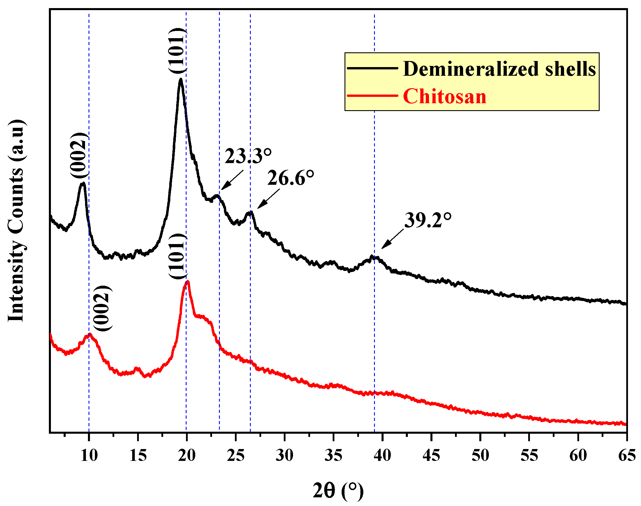
3.1.1. Characterization of Prepared Chitosan via XRD

The XRD patterns of the chitosan showed strong reflections at 2θ of around 9° and 10° and at 2θ of 20° and 21°. The distinct crystalline reflections can be attributed to the presence of plenty of hydroxyl and amino groups existing in the chitosan structure.
The characteristic peaks of chitosan centered at 10° and 20° in 2θ, which are presented in Figure 1, corresponded to the crystallographic planes of (002) and (101), respectively. Similar results have been reported by Molatlhegi et al. [44] and Antonino [33].

3.1.2. Characterization of Prepared Chitosan via IR

The ATR spectra of prepared chitosan are illustrated in Figure 2. The characteristic absorption broad band at 3291.42 cm−1 could be assigned to the stretching of the O–H bond in polymers, and the N–H elongation in primary amides (free N–H) could also be due to the intermolecular H-bonds. The same results have been reported in previous works [33,44].
An adsorption band at 2873.62 cm−1 could be associated with O–H elongation in the unsaturated and aryl carboxylic acids of α and β. C–H stretching in the 2800–3000 cm−1 range demonstrated the existence of the methyl group in NHCOCH3, the methylene group in CH2OH, and the methine group in pyranose. Similar results were observed by prior studies [45]. A characteristic band of C=O integration was observed at around 1650.89 cm−1 due to partial deacetylation [44]. When the same spectrum was observed, the band from 1500–1700 was stressed, indicating that there was an intensification of the peak at 1597 cm−1 and a decrease at 1656 cm−1, which suggests the occurrence of deacetylation [45]. Also, this band is characteristic of C=C elongation and indicated the prevalence of NH2 groups (Amide I) [33]. A band recorded at 1373.53 cm−1 was attributable to C–N stretching and CH3 deformation in the symmetrical plane, which is characteristic of polysaccharides. Molatlhegi and Alagha [44] reported similar results. The IR spectra of the prepared chitosan showed several characteristic bands. At 1148.80 cm−1, there was a band due to the C–O stretching of a secondary alcohol, as well as strong elongation of the C–O in C–O–C and antisymmetric stretching of the C–O–C bridge, which are all characteristics of the saccharide structure. The last two bands indicated the presence of polysaccharides. Another band was observed at 1025.12 cm−1, which was related to the elongation of C–N in primary, secondary, and tertiary aliphatic amines. This band could also be assigned to the C–O stretching of a primary alcohol and to O–H bending [45]. Two additional bands at 892.95 cm−1 and 593.39 cm−1 were attributed to the trisubstituted meta or disubstituted meta aromatic C–H bond and the strong elongation of C–Cl, respectively [33,44,46]

3.1.3. Point of Zero Charge (pHpzc)

The pH of the zero-charge point of chitosan was equal to 8.0 (Figure S2). Beyond this value, the chitosan was negatively charged, and below this value, the chitosan had a positive charge. The same results were found by Boudouaia et al. [29].

3.2. Adsorption Studies

3.2.1. Equilibrium Studies

The curves presented in Figure 3 show that the kinetics of OG fixation for the different concentrations of OG were fast at the beginning of the contact between the adsorbate and the adsorbent (in the first five minutes). After this time and until 420 min, the maximum capacities obtained at initial concentrations of OG of 10, 30, 50, 70, and 90 mg/L were 8.74 mg/g at 90 min, 18.20 mg/g at 210 min, 30.62 mg/g at 270 min, 31.75 mg/g, and 31.9 at 420 min, respectively. These curves can be divided into two parts: the first one from t = 0 min to t = 420 min corresponding to a fast increase in the adsorbed quantity with the increase in the OG concentration. Beyond 420 min, the adsorption reached equilibrium, and the adsorbed quantity remained constant for the different concentrations.

3.2.2. Effect of Key Parameters on the OG Adsorption

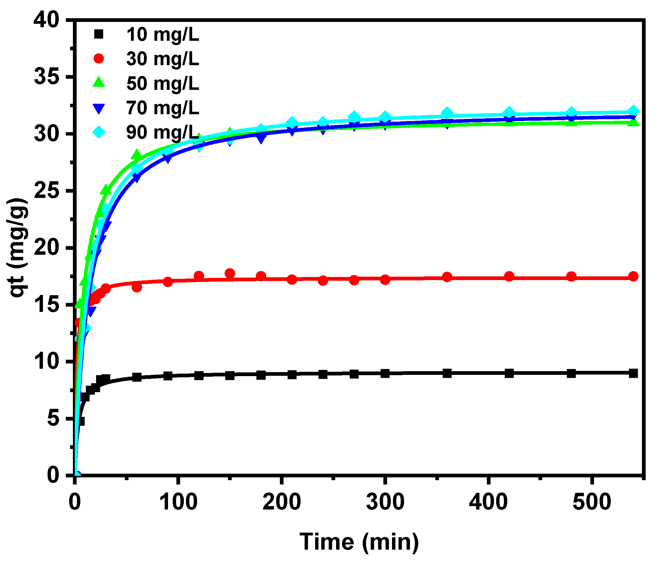
Effect of OG Concentration and Contact Time

The adsorption capacity increased with the increase in the initial concentration of the dye (Figure 3). This value passed from 8.74 mg/g for the concentration of 10 mg/L to the value of 30.62 mg/g for the concentration of 50 mg/g and reached 31.9 mg/g at 90 mg/L. The initial concentration of solute acts as a driving force for the adsorption process, favoring diffusion and mass transfer processes from the solution (with a higher amount of dye) to the free surface of the adsorbent [47,48]. The adsorption capacity of OG dye onto prepared chitosan increased with increasing contact time and reached a plateau at 420 min for high concentrations (Figure 3). This is very important to know for the stirring time for adsorption tests.

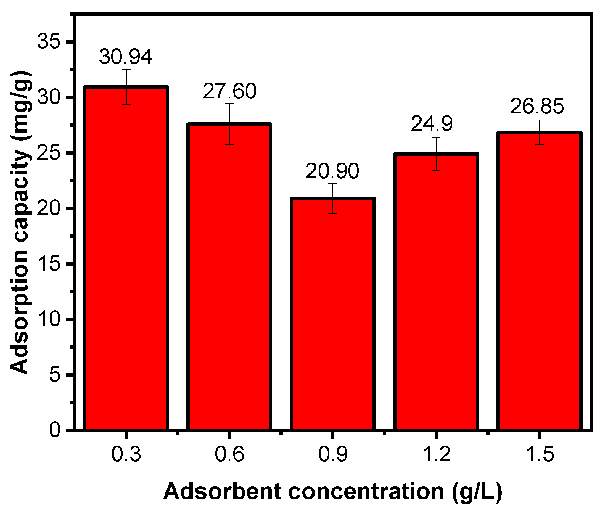
Effect of Chitosan Concentration

It is clearly represented in Figure 4 that the adsorption capacity of Orange G dye slowly decreased with the mass of the adsorbent in the mass range between 0.3 and 0.9 g/L, (from 31 mg/g to 21 mg/g). After that, it increased proportionally with this dose up to 27 mg/g at 1.5 g/L. As the concentration of adsorbent increased, the adsorption capacity efficiency of the pollutants increased, but there was no direct proportionality between the amount of adsorbent and the amount of pollutant removed. This can be attributed to the fact that the shape of the sorption isotherm changed with increasing biosorbent concentration [49].

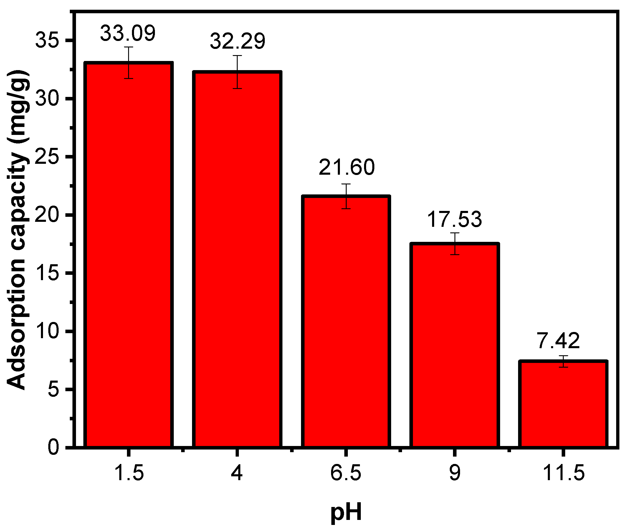
Effect of Solution pH

Figure 5 and Figure 6 illustrate the effect of solution pH on the OG adsorption and the various interactions between the chitosan and Orange G surfaces, including electrostatic attraction and hydrogen bonding, at a solution pH ˂ 8, respectively.
Figure 6 shows a rapid drop in the adsorption capacity with increasing pH, from 33 mg/g at an acid pH to 21.6 mg/g at a neutral pH, and this decrease continued until an alkaline pH. Since the pHpzc value of chitosan was 8, (Figure S2), at pH < pHpzc, the surface of the adsorbent was predominantly positive, and since OG is an anionic dye, the maximum adsorbed amount was noted at a very acidic pH. Similar results have been reported in several studies [50,51]. Under acidic conditions, the amine groups (–NH2) of chitosan could be protonated by H+ in the solution; in addition, Orange G was dissolved in the aqueous solution, and its sulfonate groups were dissociated, as illustrated in Figure 5.
The adsorption process could then proceed due to electrostatic interactions between the protonated amino groups of chitosan and the anionic sulfonic groups of dye. Additionally, the adsorption mechanism for chitosan involved n–π interactions between the orbitals of the aromatic group in the OG dye and the electrons of oxygen atoms of chitosan. The adsorption sites increased with decreasing solution pH due to the protonation of more amino groups of chitosan, which suggests that the adsorption capacity of Orange G by chitosan increased [52]. However, at higher pH, the dye removal efficiency decreased, which can be attributed to the reduction in dye dissociation resulting in a lower concentration of anionic dye available to interact with chitosan. At high pH, the amount of protonated amino groups decreased, and more OH ions were available to compete with the anionic sulfonic groups, so dye removal decreased at high pH [53].

Effect of Temperature on Adsorption Capacity

The decrease in adsorption capacity with increasing temperature obtained was due to the degradation of the structure of the biosorbent. In this study, physical adsorption occurred, owing to the negative impact when temperature was increased (Figure 7). Temperature can chemically alter an adsorbent, its adsorption sites, and its activity [14]. With increasing temperature, the adsorption process (efficiency) decreased. This can be explained by the fact that the adsorption powers between the adsorbate and the active sites of the adsorbent weakened with increasing temperature, and the efficiency of the adsorption capacity decreased [54] in accordance with exothermic adsorption. Due to the interactive natures of multiple experimental conditions on the specific dye and adsorbent being investigated, it was not feasible to establish a definitive and universally applicable effect for each parameter. For this purpose, a design of experiment method was necessary to study the effect of each factor and the interactions between them.

3.2.3. Adsorption Kinetics Modeling

In this study, two kinetics models were applied to investigate the kinetic data of the Orange G adsorption onto the prepared chitosan, including the Lagergren’s pseudo-first-order and the pseudo-second-order models, which are commonly used to describe adsorption data. The experimental data were well-adapted with the pseudo-second-order model [55]:
d q t d t = k 2 q e q t 2
The integration of this equation for the boundary conditions of (t = 0, qt = 0) with the amount of dye adsorbed being qt for any time t after rearranging the corresponding rate law, can obtain the following:
q t = q e 2   k 2   t q e k 2   t + 1
where k2 (g/mg·min) is the pseudo-second-order rate constant.
The pseudo-second-order treatment using the nonlinear model was applied, and the error distribution in the prediction of the model parameters was evaluated using the Chi-squared function ( χ 2). The fitness of the model to the experimental data was assessed using the coefficient of determination (R2).
The following mathematical equations were used for evaluating the error functions [56]:
χ 2 = ( q e , e x p q c a l c ) 2 q e , c a l c
R 2 = 1 q e , e x p q e , c a l c 2 q e , e x p q m e a n 2
where qe,exp is the experimental value of q measured at equilibrium, qe,calc is the fitted value of q, and qe,mean is the mean value of the experimental q. The closer R2 is to unity, the better the fitting quality. In Equations (8) and (9), if the qe,calc using a model is similar to the qe,exp, then χ 2 is close to zero. High χ 2 values indicate a high bias between the experimental data and the tested model [57].
The parameters obtained for the pseudo-second-order model are given in Table 2 for different dye concentrations.

3.2.4. Adsorption Isotherms

Adsorption isotherms describe how adsorbates interact with adsorbents and are essential for optimizing adsorbent use. Two isotherms, the Langmuir isotherm and the Freundlich isotherm, were evaluated for their capacity to characterize the experimental data.

Langmuir Isotherm

The Langmuir adsorption model is based on the assumption that maximum adsorption corresponds to a saturated monolayer of solute molecules on the adsorbent surface. The Langmuir isotherm model equation is presented as follows [58]:
q e = q m K L C e 1 + K L C e
where qe (mg/g) and Ce (mg/L) are the amount of adsorbed Orange G per unit mass of adsorbent and the OG concentration at equilibrium, respectively. qm is the maximum amount of OG per unit mass of adsorbent needed to form a complete monolayer on the surface bound at high Ce, and KL is a constant related to the affinity of the binding sites. The main properties of the Langmuir isotherm may be described in terms of a dimensionless constant separation factor RL, which is provided with the following equation:
R L = 1 1 + K L . C 0
where C0 is the highest initial concentration of the adsorbate (mg/L) and KL (L/mg) is the Langmuir constant. The value of RL indicates the shape of the isotherm to be either unfavorable (RL > 1), linear (RL = 1), favorable (0 < RL < 1), or irreversible (RL = 0).

Freundlich Isotherm

The Freundlich isotherm demonstrates the relationship between an equilibrium liquid and solid phase capacity based on multilayer adsorption, and it is an empirical equation used to represent heterogeneous systems (heterogeneous surface). The Freundlich isotherm is provided by the following:
q e = K f ( C e ) 1 n
where Kf and n are Freundlich constants, Kf (mg/g (L/mg)1/n) is the adsorption capacity of the sorbent, and n is a constant indicating the favorability of the adsorption process. Values of n > 1 represent favorable adsorption conditions [59].
The values of the Langmuir and Freundlich constants were calculated using the nonlinearized model (Figure 8) and are listed in Table 3.
Table 3 shows the isotherms constants and regression coefficients. The values of R2 and χ 2 were greater for the Langmuir isotherm than for the Freundlich isotherm, indicating that the Langmuir equation accurately represented the adsorption process. This might be owing to the uniform distribution of active sites on the chitosan surface. The RL = 0.044 value was between 0 and 1, showing that OG adsorption by chitosan was favorable. Table 3 shows that the Langmuir isotherm fitted the experimental data quite well (R2 = 0.998), and the monolayer adsorption capacity according to this model was 34.63 mg/g for the Langmuir isotherm, which could be compared to the experimental qmax (31.9 mg/g). The maximum adsorption capacity of the generated adsorbent was comparable to those of other low-cost adsorbents studied in the literature for the removal of anionic dyes (Table 4). The results suggest that shrimp carapace-derived chitosan is a convenient adsorbent, competitive with several other reported materials.

3.3. Data Analysis via Response Surface Methodology

In our study, the design of experiments method for the optimization and modeling of the adsorption processes of Orange G dye onto chitosan prepared from shrimp shells was applied. Five input variables (factors), with each factor taking five levels, were considered. The output variable (response) was the percentage of removal. Table 5 gathers the studied factors with their real and coded levels.
The distance of α = (2K−1)1/4 = (24)1/4 = 2 and the combination of these factors following JMP software gave N = 2K−1 +2K + n0 = 24 + 2.5 + 3 = 29 manipulations, which are presented in Table 6.
Regarding the experimental model, three complements must be considered. The first complement is the significant index (the probability p). According to Goupy and Creighton [39], if p is less than 0.05, the factor is significant. If p is less than 0.01, the factor is very significant. If p is less than 0.001, the factor is very highly significant. The second complement is the “lack of fit”. This expression expresses the fact that an a priori model is most probably different from the real model, which governs the studied phenomenon. There is a gap between these two models. This gap is the lack of fit, or RADj. The third complement is the random nature of the response. Indeed, if a response is measured several times at the same experimental point, the same result is not exactly obtained. The results are dispersed. The dispersions thus observed are called experimental errors and are noted as e (e < 5: insignificant error) [39]. Table 7 and Figure S3 show that the model obtained was very highly significant (p < 0.0001), and the agreement between the percentage of removal (yield %) predicted and the corresponding experimental data was very strong. The clouds of experimental points were very close to the line (the model), which confirmed the robustness of the model with an R2 = 0.98. The RADj of the model was 0.95, which means that the postulated model was well-fitted to the real model, and the root mean square error (RMSE) was equal to 2.5759, which was below 5%, indicating the validity of the model.

3.3.1. Analysis of Variance

The study of the significance of the factors, as well as of the interactions, was established by the ANOVA option proposed by the JMP software. The results presented in Table 7 show that the pH (X3) had a very highly significant effect (p ˂ 0.0001) with F = 82.56, followed by temperature (with p = 0.0005 and F = 31.01), while the other three factors did not have a significant effect on the percentage of OG dye removal by the prepared chitosan. Table 7 illustrates the significant interactive terms of (X1X2), (X2X3), (X3X5), (X1X4), and (X4X5). Regression analysis data indicated that the quadratic terms of X22, X32, and X55 were also significant.

3.3.2. Mathematical Modeling

The relationships between the experimental response for removal (yield %) and the five variables could be determined using the parameter estimates. The obtained results showed a positive effect for the initial concentration of OG; on the other hand, the four other variables negatively influenced the adsorption. A direct and significant interaction between pH (X3) and time (X4) could be noticed, but the other significant interactive terms were negative and had an inverse effect (initial concentration of OG and pH (X1X3), initial concentration of OG and time (X1X4), time and temperature (X4X5)). The significant coefficients of quadratic terms of X22, X32, and X52 had a positive effect on the adsorbed quantity of OG, while the other interactions had no significant effect.
Finally, the OG removal yield by the chitosan prepared from shrimp shells could be predicted with the following equation:
R e m o v a l   % = 7.053 7.241 X 3 4.438 X 5 + 2.88 X 1 X 2 4.098 X 1 X 4 2.581 X 2 X 3 + 2.342 X 3 X 5 4.648 X 4 X 5 + 2.34 X 2 2 + 3.342   X 3 2 + 2.979   X 5 2 + 3.904

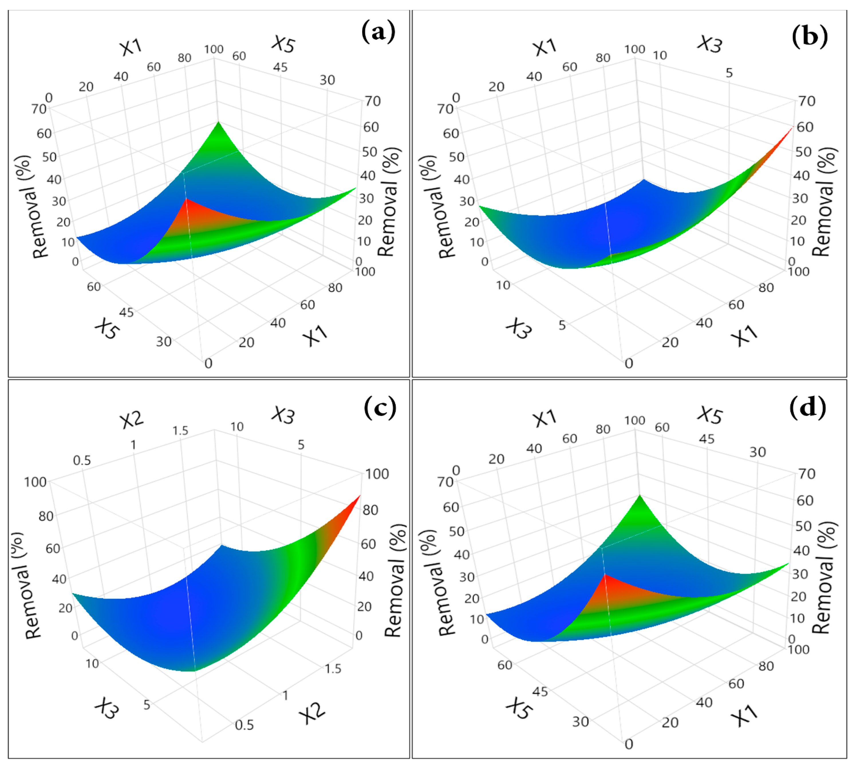
3.3.3. RSM Evolution

Response surfaces can show the variations in responses as a function of only two factors at a time. Figure 9a shows the response surface of the percentage of removal as a function of initial OG dye concentration and adsorbent concentration. This graph shows a positive interaction between these two factors with removal = 50% at maximum values of OG and adsorbent concentration. Figure 9b represents the response surface of the percentage of removal as a function of dye concentration and pH. A maximum removal rate equal to 60% was observed at the maximum upper bound of the concentration corresponding to the minimum pH value. From Figure 9c, it can be deduced that a removal of 70% for the minimum pH value and the maximum concentration value of the adsorbent was achieved. A removal value of 60% could be noticed for the two minimal values of temperature and concentration of the adsorbent (Figure 9d).

3.3.4. Optimization of the Values of the Variables

To establish the values of the variables maximizing the percentage of removal of OG dye by chitosan prepared from shrimp shells, the optimization diagram obtained using the maximum desirability function (D = 1) proposed by JMP® Pro statistical software version 13.2.1 was used. In separate columns, the response is related to each of the five factors: the vertical red dashed lines show the values of the factors, while the horizontal ones show the response for the selected factor levels. In Figure S4, the simulation was adjusted to maximize the removal (%), and the statistical sweet spot was determined for a maximum removal of 97.43% and a desirability of d = 1.0, leading to C0 = 10 mg/L, S/L = 0.3 g/L, pH = 6.5, temperature = 25 °C, and contact time = 450 min.

3.4. Thermodynamic Studies

The thermodynamic study of any adsorption process provides information on the energy changes and shows whether the process is spontaneous or not [67]. It is essential for predicting the adsorption mechanisms. In our study, the thermodynamics of the adsorption process were examined at five different temperatures from 298.18 K to 338.15 K. Thermodynamic factors, such as Gibbs free energy change (∆G0), the change in enthalpy (ΔH0), and the change in entropy (ΔS0), were evaluated using the Van’t Hoff equation [68]:
G 0 = RT ln ( K L 0 )  
where R = 8.314 J/mol·K is the universal gas constant, T is the absolute temperature (K), and KL0 is the (dimensionless) ‘thermodynamic’ Langmuir constant for the adsorption process calculated from KL (L/mg) in the Langmuir model after changing all concentrations to molar form and considering the standard state of C0 = 1 mol/L [68]:
K L 0 = K L L m g · 1000 m g g · M O G g m o l · C 0 m o l L
where M = 452.386 g/mol, or the molar mass of Orange G; and the factor 1000 converts g to mg. The enthalpy (ΔH0) and entropy (ΔS0) parameters were estimated from the classical relationships:
ln K L 0 = ( S 0 / R ) ( H 0 / RT )  
G 0 = H 0 T S 0
The plot of lnKL0 versus 1/T yielded a straight line, and the values of ∆H0 (kJ/mol) and ∆S0 (J/mol K) can be calculated from the intercept and slope of these Van’t Hoff plots, respectively. The values of ∆G0 (kJ/mol) were recalculated from ∆H° and ∆S0 (Table 8). The negative values of ∆H0 were indicative of an exothermic adsorption. The negative values of ∆G0 demonstrated that the present chitosan adsorbent was effective in the removal of Orange G dye from the aqueous phase.

4. Conclusions

In the present study, Chitosan was synthesized from shrimp shells using a hydrothermochemical process. The results obtained via the FTIR spectra showed that the adsorbent’s functional groups, especially the O-H, C-C, and C-H stretch bands, were involved with dye adsorption. The highest adsorbed amount was 31.9 mg/g (removal = 45%) for an initial adsorbate concentration of C0 = 90 mg/L, a pH = 6.5, a T = 25 °C, an adsorbent concentration of S/L = 0.9 g/L, and 420 min of contact time.
The adsorption kinetic data were evaluated and the pseudo-second order model was most representative. The adsorption equilibrium was studied using two nonlinear forms of adsorption isotherms: Langmuir and Freundlich. The Langmuir model showed good adsorption, with a maximum adsorption capacity of 34.63 mg/g.
Response surface methodology and a central composite rotatable design were utilized to assess the influence of initial OG concentration, pH, chitosan amount, temperature, and contact time on the percentage of removal of OG by synthesized chitosan. This response was modeled with a second-degree polynomial equation. The optimal percentage of removal was 97.43% for an initial concentration of OG of 10 mg/L, a pH of 6.5, an S/L = 0.3 g/L, a temperature of 25 °C, and 450 min of adsorption time.
The thermodynamics studies showed that the adsorption system was spontaneous with an exothermic character. The chitosan produced from shrimp carapaces may be environmentally friendly and efficiently used to treat wastewater. The three potential processes that could control the adsorption of OG by chitosan were electrostatic forces, n–π interaction, and H bonding. I have chicked
The study of the elimination of Orange G dye, which is a very toxic product dissolved in water, using ecofriendly chitosan showed us that chitosan is a good biosorbent of this anionic dye. For this purpose, we are very interested in exploiting this investigation for the elimination of real industrial effluents and targeting the chitosan regeneration mechanism.

Supplementary Materials

The following supporting information can be downloaded at: https://www.mdpi.com/article/10.3390/w15213728/s1. Figure S1. Preparation steps of chitosan. Figure S2. pHpzc of the prepared chitosan. Figure S3. Graphs of observed values of adsorption capacity versus predicted values. Figure S4. Diagrammatic optimization of Orange G removal parameters.

Author Contributions

Conceptualization, K.B., N.B., A.I. and L.M.; software, A.I.; methodology, K.B., L.M., H.Z. and N.B. validation, A.I., L.M. and A.A.; formal analysis, K.B. and A.I.; investigation, K.B.; resources, A.I., N.B., H.Z., L.M. and A.A.; data curation, K.B. and L.M.; writing—original draft preparation, J.-C.B., A.A.A. and K.B.; writing—review and editing, K.B., L.M., H.Z., J.-C.B. and A.A.; visualization, L.M., A.A.A., J.-C.B. and A.A.; supervision, L.M. and A.A.; project administration, L.M., A.A.A. and A.A. All authors have read and agreed to the published version of the manuscript.

Funding

This work was funded by the Directorate-General for Scientific Research and Technological Development (DGRSDT).

Data Availability Statement

Not applicable.

Acknowledgments

The authors would like to thank the Directorate-General for Scientific Research and Technological Development (DGRSDT) for supporting this work.

Conflicts of Interest

The authors declare no conflict of interest.

References

  1. Pokhrel, D.; Viraraghavan, T. Treatment of Pulp and Paper Mill Wastewater—A Review. Sci. Total Environ. 2004, 333, 37–58. [Google Scholar] [CrossRef] [PubMed]
  2. Javadinejad, S.; Dara, R.; Hamed, M.; Akram, M.; Saeed, H.; Jafary, F. Analysis of Gray Water Recycling by Reuse of Industrial Waste Water for Agricultural and Irrigation Purposes. J. Geogr. Res. 2020, 3, 20–24. [Google Scholar] [CrossRef]
  3. Le, T.T.; Nguyen, T.; Nguyen, Q.; Man, P.; Kim, K.; Nguyen, N.H. Orange G Degradation by Heterogeneous Peroxymonosulfate Activation Based on Magnetic MnFe2O4/α-MnO2 Hybrid. J. Environ. Sci. 2023, 124, 379–396. [Google Scholar] [CrossRef]
  4. Boudraa, R.; Talantikite-Touati, D.; Souici, A.; Djermoune, A.; Saidani, A.; Fendi, K.; Amrane, A.; Bollinger, J.-C.; Tran, H.N.; Hadadi, A. Optical and Photocatalytic Properties of TiO2–Bi2O3–CuO Supported on Natural Zeolite for Removing Safranin-O Dye from Water and Wastewater. J. Photochem. Photobiol. A Chem. 2023, 443, 114845. [Google Scholar] [CrossRef]
  5. Patel, H.; Yadav, V.K.; Yadav, K.K.; Choudhary, N.; Kalasariya, H.; Alam, M.M.; Gacem, A.; Amanullah, M.; Ibrahium, H.A.; Park, J.-W. A Recent and Systemic Approach Towards Microbial Biodegradation of Dyes from Textile Industries. Water 2022, 14, 3163. [Google Scholar] [CrossRef]
  6. Hadadi, A.; Imessaoudene, A.; Bollinger, J.-C.; Assadi, A.A.; Amrane, A.; Mouni, L. Comparison of Four Plant-Based Bio-Coagulants Performances against Alum and Ferric Chloride in the Turbidity Improvement of Bentonite Synthetic Water. Water 2022, 14, 3324. [Google Scholar] [CrossRef]
  7. Hadadi, A.; Imessaoudene, A.; Bollinger, J.-C.; Cheikh, S.; Assadi, A.A.; Amrane, A.; Kebir, M.; Mouni, L. Parametrical Study for the Effective Removal of Mordant Black 11 from Synthetic Solutions: Moringa Oleifera Seeds’ Extracts Versus Alum. Water 2022, 14, 4109. [Google Scholar] [CrossRef]
  8. Gupta, V.; Kumar, R.; Nayak, A.; Saleh, T.; Barakat, M. Adsorptive Removal of Dyes from Aqueous Solution onto Carbon Nanotubes: A Review. Adv. Colloid. Interface Sci. 2013, 193, 24–34. [Google Scholar] [CrossRef]
  9. Lan, D.; Zhu, H.; Zhang, J.; Li, S.; Chen, Q.; Wang, C.; Wu, T.; Xu, M. Adsorptive Removal of Organic Dyes via Porous Materials for Wastewater Treatment in Recent Decades: A Review on Species, Mechanisms and Perspectives. Chemosphere 2022, 293, 133464. [Google Scholar] [CrossRef]
  10. Imessaoudene, A.; Cheikh, S.; Bollinger, J.-C.; Belkhiri, L.; Tiri, A.; Bouzaza, A.; El Jery, A.; Assadi, A.; Amrane, A.; Mouni, L. Zeolite Waste Characterization and Use as Low-Cost, Ecofriendly, and Sustainable Material for Malachite Green and Methylene Blue Dyes Removal: Box–Behnken Design, Kinetics, and Thermodynamics. Appl. Sci. 2022, 12, 7587. [Google Scholar] [CrossRef]
  11. Mouni, L.; Belkhiri, L.; Bollinger, J.-C.; Bouzaza, A.; Assadi, A.; Tirri, A.; Dahmoune, F.; Madani, K.; Remini, H. Removal of Methylene Blue from Aqueous Solutions by Adsorption on Kaolin: Kinetic and Equilibrium Studies. Appl. Clay Sci. 2018, 153, 38–45. [Google Scholar] [CrossRef]
  12. Bouchelkia, N.; Tahraoui, H.; Amrane, A.; Belkacemi, H.; Bollinger, J.-C.; Bouzaza, A.; Zoukel, A.; Zhang, J.; Mouni, L. Jujube Stones Based Highly Efficient Activated Carbon for Methylene Blue Adsorption: Kinetics and Isotherms Modeling, Thermodynamics and Mechanism Study, Optimization via Response Surface Methodology and Machine Learning Approaches. Process Saf. Environ. Prot. 2023, 170, 513–535. [Google Scholar] [CrossRef]
  13. Chedri Mammar, A.; Mouni, L.; Bollinger, J.-C.; Belkhiri, L.; Bouzaza, A.; Assadi, A.A.; Belkacemi, H. Modeling and Optimization of Process Parameters in Elucidating the Adsorption Mechanism of Gallic Acid on Activated Carbon Prepared from Date Stones. Sep. Sci. Technol. 2020, 55, 3113–3125. [Google Scholar] [CrossRef]
  14. Rápó, E.; Tonk, S. Factors Affecting Synthetic Dye Adsorption; Desorption Studies: A Review of Results from the Last Five Years (2017–2021). Molecules 2021, 26, 5419. [Google Scholar] [CrossRef] [PubMed]
  15. Chang, M.-Y.; Juang, R.-S. Adsorption of Tannic Acid, Humic Acid, and Dyes from Water Using the Composite of Chitosan and Activated Clay. J. Colloid. Interface Sci. 2004, 278, 18–25. [Google Scholar] [CrossRef] [PubMed]
  16. Miretzky, P.; Cirelli, A. Fluoride Removal from Water by Chitosan Derivatives and Composites. J. Fluor. Chem. 2011, 132, 231–240. [Google Scholar] [CrossRef]
  17. Gul, K.; Sohni, S.; Waqar, M.; Ahmad, F.; Norulaini, N.; Kadir, M. Functionalization of Magnetic Chitosan with Graphene Oxide for Removal of Cationic and Anionic Dyes from Aqueous Solution. Carbohydr. Polym. 2016, 152, 520–531. [Google Scholar] [CrossRef] [PubMed]
  18. Guo, P.; Anderson, J.; Bozell, J.; Zivanovic, S. The Effect of Solvent Composition on Grafting Gallic Acid onto Chitosan via Carbodiimide. Carbohydr. Polym. 2016, 140, 171–180. [Google Scholar] [CrossRef] [PubMed]
  19. Zhai, L.; Bai, Z.; Zhu, Y.; Wang, B.; Luo, W. Fabrication of Chitosan Microspheres for Efficient Adsorption of Methyl Orange. Chin. J. Chem. Eng. 2018, 26, 657–666. [Google Scholar] [CrossRef]
  20. Kumar, M. A Review of Chitin and Chitosan Applications. React. Funct. Polym. 2000, 46, 1–27. [Google Scholar] [CrossRef]
  21. Xu, Y.; Li, L.; Cao, S.; Zhu, B.; Yao, Z. An Updated Comprehensive Review of Advances on Structural Features, Catalytic Mechanisms, Modification Methods and Applications of Chitosanases. Process Biochem. 2022, 118, 263–273. [Google Scholar] [CrossRef]
  22. Hahn, T.; Roth, A.; Ji, R.; Schmitt, E.; Zibek, S. Chitosan Production with Larval Exoskeletons Derived from the Insect Protein Production. J. Biotechnol. 2020, 310, 62–67. [Google Scholar] [CrossRef] [PubMed]
  23. Spranghers, T.; Ottoboni, M.; Klootwijk, C.; Ovyn, A.; Deboosere, S.; Meulenaer, B.; Michiels, J.; Eeckhout, M.; De Clercq, P.; De Smet, S. Nutritional Composition of Black Soldier Fly (Hermetia Illucens) Prepupae Reared on Different Organic Waste Substrates. J. Sci. Food Agric. 2017, 97, 2594–2600. [Google Scholar] [CrossRef] [PubMed]
  24. Loc, N.; Tuyen, P.; Mai, L.; Phuong, D. Chitosan-Modified Biochar and Unmodified Biochar for Methyl Orange: Adsorption Characteristics and Mechanism Exploration. Toxics 2022, 10, 500. [Google Scholar] [CrossRef]
  25. Iber, B.; Kasan, N.; Torsabo, D.; Omuwa, J. A Review of Various Sources of Chitin and Chitosan in Nature. J. Renew. Mater. 2021, 10, 42–49. [Google Scholar] [CrossRef]
  26. Durakovic, B. Design of Experiments Application, Concepts, Examples: State of the Art. Period. Eng. Nat. Sci. 2017, 5, 421–439. [Google Scholar] [CrossRef]
  27. Osborne, D.M.; Armacost, R.L.; Pet-Edwards, J. State of the Art in Multiple Response Surface Methodology. In Proceedings of the 1997 IEEE International Conference on Systems, Man, and Cybernetics. Computational Cybernetics and Simulation, Orlando, FL, USA, 12–15 October 1997; Volume 4, p. 3838, ISBN 0-7803-4053-1. [Google Scholar]
  28. Truong, T.; Hausler, R.; Monette, F.; Niquette, P. The Valorization of Industrial Fishery Waste through the Hydrothermal-Chemical Transformation of Chitosan. Rev. Sci. L’Eau 2007, 20, 253–262. [Google Scholar] [CrossRef]
  29. Boudouaia, N.; Bengharez, Z.; Jellali, S. Preparation and Characterization of Chitosan Extracted from Shrimp Shells Waste and Chitosan Film: Application for Eriochrome Black T Removal from Aqueous Solutions. Appl. Water Sci. 2019, 9, 91. [Google Scholar] [CrossRef]
  30. Meetani, M.; Rauf, M.; Hisaindee, S.; Khaleel, A.; Alzamly, A.; Ahmad, A. Mechanistic Studies of Photoinduced Degradation of Orange G Using LC/MS. RSC Adv. 2011, 1, 490–497. [Google Scholar] [CrossRef]
  31. Li, Y.; Yang, Z.; Zhang, H.; Tong, X.; Feng, J. Fabrication of Sewage Sludge-Derived Magnetic Nanocomposites as Heterogeneous Catalyst for Persulfate Activation of Orange G Degradation. Colloids Surf. Physicochem. Eng. Asp. 2017, 529. [Google Scholar] [CrossRef]
  32. Mondal, M.; Singh, S.; Umareddy, M.; Dasgupta, B. Removal of Orange G from Aqueous Solution by Hematite: Isotherm and Mass Transfer Studies. Korean J. Chem. Eng. 2010, 27, 1811–1815. [Google Scholar] [CrossRef]
  33. Antonino, R.; Fook, B.; Lima, V.; Farias, R.; Lima, E.; Lima, R.; Covas, C.; Lia Fook, M. Preparation and Characterization of Chitosan Obtained from Shells of Shrimp (Litopenaeus Vannamei Boone). Mar. Drugs 2017, 15, 141. [Google Scholar] [CrossRef]
  34. Fiol, N.; Villaescusa, I. Determination of sorbent point zero charge: Usefulnessin sorption studies. Environ. Chem. Lett. 2009, 7, 79–84. [Google Scholar] [CrossRef]
  35. Imessaoudene, A.; Cheikh, S.; Hadadi, A.; Hamri, N.; Bollinger, J.-C.; Amrane, A.; Tahraoui, H.; Manseri, A.; Mouni, L. Adsorption Performance of Zeolite for the Removal of Congo Red Dye: Factorial Design Experiments, Kinetic, and Equilibrium Studies. Separations 2023, 10, 57. [Google Scholar] [CrossRef]
  36. Hadadi, A.; Imessaoudene, A.; Bollinger, J.-C.; Cheikh, S.; Manseri, A.; Mouni, L. Dual Valorization of Potato Peel (Solanum tuberosum) as a Versatile and Sustainable Agricultural Waste in Both Bioflocculation of Eriochrome Black T and Biosorption of Methylene Blue. J. Polym. Environ. 2023, 1–16. [Google Scholar] [CrossRef]
  37. Tinsson, W. Plans d’expérience: Constructions et Analyses Statistiques; Springer Science & Business Media: Berlin/Heidelberg, Germany, 2010; Volume 67, ISBN 3-642-11472-5. [Google Scholar]
  38. Montgomery, D.C. Desing and Analysis of Experiments; Jonh Wiley Sons Quinta: Hoboken, NJ, USA, 2001. [Google Scholar]
  39. Goupy, J.; Creighton, L. Introduction Aux Plans d’expériences: Avec Applications; Dunod: Paris, France, 2013; ISBN 2-10-059296-3. [Google Scholar]
  40. Granato, D.; de Araújo Calado, V.M.; Jarvis, B. Observations on the Use of Statistical Methods in Food Science and Technology. Food Res. Int. 2014, 55, 137–149. [Google Scholar] [CrossRef]
  41. Pillet, M. Les Plans d’expériences Par La Méthode Taguchi; Editions d’Organisation: New York, NY, USA, 2001. [Google Scholar]
  42. Bhattacharya, S. Central Composite Design for Response Surface Methodology and Its Application in Pharmacy. In Response Surface Methodology in Engineering Science; IntechOpen: London, UK, 2021; pp. 1–19. ISBN 978-1-83968-917-8. [Google Scholar]
  43. Khoder, K. Optimisation de Composants Hyperfréquences Par La Technique Des Plans à Surfaces de Réponses. Limoges University. 2011. Available online: https://aurore.unilim.fr/ori-oai-search/notice/view/unilim-ori-28713 (accessed on 14 September 2023).
  44. Molatlhegi, O.; Alagha, L. Adsorption Characteristics of Chitosan Grafted Copolymer on Kaolin. Appl. Clay Sci. 2017, 150, 342–353. [Google Scholar] [CrossRef]
  45. Kumari, S.; Rath, P. Extraction and Characterization of Chitin and Chitosan from (Labeo Rohit) Fish Scales. Procedia Mater. Sci. 2014, 6, 482–489. [Google Scholar] [CrossRef]
  46. Povea, M.; Argüelles-Monal, W.; Valerio, J.; Rodríguez, C.; May Pat, A.; Rivero, N.; Peniche, C. Interpenetrated Chitosan-Poly(acrylic acid-co-acrylamide) Hydrogels. Synthesis, Characterization and Sustained Protein Release Studies. Mater. Sci. Appl. 2011, 2, 509–520. [Google Scholar] [CrossRef]
  47. Al-Ghouti, M.A.; Da’ana, D.A. Guidelines for the Use and Interpretation of Adsorption Isotherm Models: A Review. J. Hazard. Mater. 2020, 393, 122383. [Google Scholar] [CrossRef]
  48. Lee, B.H.; Lum, N.; Seow, L.; Lim, P.; Tan, L.P. Synthesis and Characterization of Types A and B Gelatin Methacryloyl for Bioink Applications. Materials 2016, 9, 797. [Google Scholar] [CrossRef] [PubMed]
  49. Dehghani, M.H.; Hassani, A.; Karri, R.; Younesi, B.; Shayeghi, M.; Salari, M.; Zarei, A.; Yousefi, M.; Heidarinejad, Z. Process Optimization and Enhancement of Pesticide Adsorption by Porous Adsorbents by Regression Analysis and Parametric Modelling. Sci. Rep. 2021, 11, 11719. [Google Scholar] [CrossRef]
  50. Venugopal, V. Seaweed, Microalgae, and Their Polysaccharides: Food Applications. In Marine Polysaccharides: Food Applications; CRC Press: Boca Raton, FL, USA, 2011; pp. 191–236. [Google Scholar]
  51. Mu’azu, N.D.; Jarrah, N.; Zubair, M.; Manzar, M.S.; Kazeem, T.S.; Qureshi, A.; Haladu, S.A.; Blaisi, N.I.; Essa, M.H.; Al-Harthi, M.A. Mechanistic Aspects of Magnetic MgAlNi Barium-Ferrite Nanocomposites Enhanced Adsorptive Removal of an Anionic Dye from Aqueous Phase. J. Saudi Chem. Soc. 2020, 24, 715–732. [Google Scholar] [CrossRef]
  52. Cheung, A.; Szeto, Y.S.; Mckay, G. Enhancing the Adsorption Capacities of Acid Dyes by Chitosan Nano Particles. Bioresour. Technol. 2008, 100, 1143–1148. [Google Scholar] [CrossRef]
  53. Zhou, L.; Jin, J.; Liu, Z.; Liang, X.; Shang, C. Adsorption of Acid Dyes from Aqueous Solutions by the Ethylenediamine-Modified Magnetic Chitosan Nanoparticles. J. Hazard. Mater. 2010, 185, 1045–1052. [Google Scholar] [CrossRef] [PubMed]
  54. Abualnaja, K.M.; Alprol, A.E.; Abu-Saied, M.A.; Ashour, M.; Mansour, A. Removing of Anionic Dye from Aqueous Solutions by Adsorption Using of Multiwalled Carbon Nanotubes and Poly (Acrylonitrile-Styrene) Impregnated with Activated Carbon. Sustainability 2021, 13, 7077. [Google Scholar] [CrossRef]
  55. Moussout, H. Critical of Linear and Nonlinear Equations of Pseudo-First Order and Pseudo-Second Order Kinetic Models. Karbala Int. J. Mod. Sci. 2018, 4, 244–254. [Google Scholar] [CrossRef]
  56. Huang, W.-Y.; Li, D.; Liu, Z.-Q.; Tao, Q.; Zhu, Y.; Yang, J.; Zhang, Y.-M. Kinetics, Isotherm, Thermodynamic, and Adsorption Mechanism Studies of La(OH)3-Modified Exfoliated Vermiculites as Highly Efficient Phosphate Adsorbents. Chem. Eng. J. 2014, 236, 191–201. [Google Scholar] [CrossRef]
  57. Vitek, R.; Masini, J. Nonlinear Regression for Treating Adsorption Isotherm Data to Characterize New Sorbents: Advantages over Linearization Demonstrated with Simulated and Experimental Data. Heliyon 2023, 9, e15128. [Google Scholar] [CrossRef]
  58. Tran, H.N.; You, S.-J.; Hosseini-Bandegharaei, A.; Chao, H.-P. Mistakes and Inconsistencies Regarding Adsorption of Contaminants from Aqueous Solutions: A Critical Review. Water Res. 2017, 120, 88–116. [Google Scholar]
  59. Tran, H.; You, S.-J.; Chao, H.-P. Fast and Efficient Adsorption of Methylene Green 5 on Activated Carbon Prepared from New Chemical Activation Method. J. Environ. Manag. 2017, 188, 322–336. [Google Scholar] [CrossRef] [PubMed]
  60. Wang, K.; Kou, Y.; Wang, K.; Liang, S.; Guo, G.; Wang, W.; Lu, Y.; Wang, J. Comparing the adsorption of methyl orange and malachite green on similar yet distinct polyamide microplastics: Uncovering hydrogen bond interactions. Chemosphere 2023, 340, 139806. [Google Scholar] [CrossRef] [PubMed]
  61. Arulkumar, M.; Sathishkumar, P.; Palvannan, T. Optimization of Orange G Dye Adsorption by Activated Carbon of Thespesia Populnea Pods Using Response Surface Methodology. J. Hazard. Mater. 2011, 186, 827–834. [Google Scholar] [CrossRef] [PubMed]
  62. Dev Vinu, V.; Wilson, B.; Nair, K.; Antony, S.; Krishnan, A. Response surface modeling of Orange-G adsorption onto surface tuned ragi husk. Colloide Interface Sci. Commun. 2021, 41, 100363. [Google Scholar] [CrossRef]
  63. Atia, A.A.; Donia, A.M.; Al-Amrani, W.A. Adsorption/Desorption Behavior of Acid Orange 10 on Magnetic Silica Modified with Amine Groups. Chem. Eng. J. 2009, 150, 55–62. [Google Scholar] [CrossRef]
  64. Potgieter, J.H.; Pardesi, C.; Pearson, S. A Kinetic and Thermodynamic Investigation into the Removal of Methyl Orange from Wastewater Utilizing Fly Ash in Different Process Configurations. Environ. Geochem. Health 2021, 43, 2539–2550. [Google Scholar] [CrossRef]
  65. Victor, R.P.; Fontes, L.L.; Neves, A.A.; de Queiroz, M.E.; Oliveira Miranda, L.D. Removal of orange G dye by manganese oxide nanostructures. J. Braz. Chem. Soc. 2019, 30, 1769–1778. [Google Scholar] [CrossRef]
  66. Rathee, V.; Awasthi, A.; Sood, D.; Tomar, R.; Tomar, V.; Chandra, R. A new biocompatible ternary layered double hydroxide adsorbent for ultrafast removal of anionic organic dyes. Sci. Rep. 2014, 9, 16225. [Google Scholar] [CrossRef]
  67. Tran, H.; Lima, E.; Juang, R.-S.; Bollinger, J.-C.; Chao, H.-P. Thermodynamic Parameters of Liquid-Phase Adsorption Process Calculated from Different Equilibrium Constants Related to Adsorption Isotherms: A Comparison Study. J. Environ. Chem. Eng. 2021, 9, 106674. [Google Scholar] [CrossRef]
  68. Salvestrini, S.; Leone, V.; Iovino, P.; Canzano, S.; Capasso, S. Considerations about the Correct Evaluation of Sorption Thermodynamic Parameters from Equilibrium Isotherms. J. Chem. Thermodyn. 2014, 68, 310–316. [Google Scholar] [CrossRef]
Figure 1. XRD spectra of prepared chitosan and demineralized shrimp shells.
Water 15 03728 g001
Figure 2. ATR spectra of crushed shells, demineralized shells, and prepared chitosan.
Water 15 03728 g002
Figure 3. Amount of OG adsorbed onto prepared chitosan as a function of time for different concentrations of OG (pH = 6.5 ± 0.1, T = 25 ± 2 °C, ratio of S/L (mass of chitosan/volume of OG dye) = 0.9 g/L, stirring speed = 200 rpm).
Water 15 03728 g003
Figure 4. Effect of adsorbent concentration on adsorption capacity (C0 = 50 mg/L, pH = 6.5, T = 25 °C, t = 240 min).
Water 15 03728 g004
Figure 5. Illustration of various interactions between the chitosan and Orange G surfaces, including electrostatic attraction and hydrogen bonding, at a solution pH ˂ 8.
Water 15 03728 g005
Figure 6. Effect of solution pH on the adsorption capacity (adsorbate concentration = 50 mg/L, S/L = 0.9 g/L, T = 25 °C, t = 240 min).
Water 15 03728 g006
Figure 7. Effect of temperature on adsorption capacity (C0 = 50 mg/L, S/L = 0.9g/L, pH = 6.5, t = 240 min).
Water 15 03728 g007
Figure 8. Nonlinearized isotherm models for OG adsorption onto prepared chitosan at pH = 6.5 ± 0.1, T = 25 °C ± 2, a ratio of mass of chitosan/volume of OG dye = 0.9 g/L, stirring speed = 200 rpm, and t = 420 min.
Water 15 03728 g008
Figure 9. 3-D response surface plots for percentage of removal of OG by prepared chitosan: (a) effect of initial concentration of OG/adsorbent concentration; (b) effect of initial concentration of OG/pH; (c) effect of adsorbent concentration/pH; (d) effect of initial concentration of OG/temperature.
Water 15 03728 g009
Table 1. Physicochemical characteristics of Orange G.
DyeOrange G
Generic nameAcid Orange 10
Commercial nameOrange G
Color index number16,230
Color Dark orange powder
ClassAzo dye
max) (nm)476
Molecular formula C16H10N2Na2O7S2
Molecular weight (g/mol)452.386
Chemical name (IUPAC)7-Hydroxy-8-(phenylazo)-1, 3-naphthalenedisulfonic acid disodium salt
Molecular structure [32]Water 15 03728 i001
Table 2. Parameters for second-order kinetic model for removal of Orange G dye at 25 °C using nonlinearized model.
C0 (mg/L)qe (exp)qe (calc)k2 (min−1)R2χ2
108.7429.088 ± 0.060.0309 0.9910.042
3018.20217.40 ± 0.080.03440.9940.083
5030.6231.48 ± 0.320.00380.9860.927
7031.7532.29 ± 0.350.00220.9880.932
903232.66 ± 0.290.00240.9910.679
Table 3. Isotherm parameters for removal of OG by prepared chitosan at 25 °C.
LangmuirFreundlich
qmax (mg/g)KL (L/mg)R2χ2KF [(mg/g)·(mg/L)1/n]1/nR2χ2
34.631 ± 0.6340. 241 ± 0.0230.9980.37912.459 ± 0.1230.262 ± 0.0030.9213.063
Table 4. Comparison of adsorption capacities of chitosan for OG with other adsorbents.
Materials Adsorption Capacity (mg/g) Reference
Polyamide 668.854[60]
Activated carbon of Thespesia populnea pods9.129[61]
Formaldehyde-modified Ragi husk14.6[62]
Magnetic silica65.89[63]
Fly ash 3.9[64]
Brown birnessite4.5[65]
Ni/Fe/Ti LDH11.81[66]
Shrimp carapace-derived chitosan34.63This study
Table 5. Studied factors with their actual and coded levels.
NoVariableNameVariable Level
−α (−2)−10+1+α (+2)
01X1C0 (mg/L)1030507090
02X2S/L (g/L)0.30.60.91.21.5
03X3pH1.546.5911.5
04X4Time (min)30135240345450
05X5Temperature (°C)25 35455565
Table 6. The uncoded CCD matrix of experiments for OG removal.
RunAdsorbate Concentration (mg/L)Adsorbent Concentration (g/L)pH Temperature Time (min)Removal (%)
ObservedPredictedResidual
1500.96.545301614.121.87
2700.69553453.50.023.47
3300.645534512.5810.831.74
4300.643513525.0825.71−0.63
5300.693534531.529.022.47
6701.245534518.3417.710.62
7500.96.5652407.210.09−2.89
8500.96.5452408.97.051.84
9301.243534540.7541.11−0.36
10500.96.52524027.8527.840.00
11301.29553455.663.851.80
12500.96.5452407.857.050.79
13500.96.5452407.37.050.24
14701.243513540.2842.03−1.75
15500.91.54524036.3634.901.45
16100.96.54524013.2514.14−0.89
17700.645513529.3528.980.36
18701.293534514.7113.351.35
19501.56.54524020.719.351.34
20500.911.5452401.65.94−4.34
21700.643534522.9221.621.29
22900.96.54524012.514.48−1.98
23500.36.5452409.2413.47−4.23
24701.295513519.4619.040.41
25700.69351357.786.691.08
26301.29351354.164.73−0.57
27300.695513515.6614.111.54
28500.96.5454503.758.504.75
29301.245513517.4118.711.30
Table 7. ANOVA for the fit of the experimental results to response surface model.
FactorDFSum of SquaresF-Valuep-Value
pH11258.6082.36<0.001
Temperature1472.7731.010.0005
C0 × S/L 1132.718.700.0184
S/L × pH1106.606.990.0295
pH × T187.795.750.0432
C0 × time1268.7917.630.003
T × time 1345.7722.680.0014
(S/L) × (S/L)1134.378.810.0179
pH × pH1274.1417.980.0028
T × T1217.7314.280.0054
Table 8. Thermodynamic parameters for Orange G adsorption by prepared chitosan.
T (K)KL (L/mg)KL0Ln KL0∆G0 (J/mol)∆H0 (kJ/mol)∆S0 (J/mol·K)
298.150.241109,02511.599−28.752
308.150.06328,500.3210.257−26.279
318.150.0230510,427.59.252−24.473−92.277−213.420
328.150.00783528.6118.168−22.286
338.150.00281266.6817.144−20.084
Disclaimer/Publisher’s Note: The statements, opinions and data contained in all publications are solely those of the individual author(s) and contributor(s) and not of MDPI and/or the editor(s). MDPI and/or the editor(s) disclaim responsibility for any injury to people or property resulting from any ideas, methods, instructions or products referred to in the content.

