Article

Using Data-Driven Prediction of Downstream 1D River Flow to Overcome the Challenges of Hydrologic River Modeling

1
Argonne National Laboratory, Environmental Science Division, 9700 S. Cass Ave., Lemont, IL 60439, USA
2
Argonne National Laboratory, Energy Systems and Infrastructure Analysis Division, 9700 S. Cass Ave., Lemont, IL 60439, USA
*
Authors to whom correspondence should be addressed.
Water 2023, 15(21), 3843; https://doi.org/10.3390/w15213843
Submission received: 9 October 2023 / Revised: 25 October 2023 / Accepted: 31 October 2023 / Published: 3 November 2023
(This article belongs to the Section Hydrology)

Abstract

:
Methods for downstream river flow prediction can be categorized into physics-based and empirical approaches. Although based on well-studied physical relationships, physics-based models rely on numerous hydrologic variables characteristic of the specific river system that can be costly to acquire. Moreover, simulation is often computationally intensive. Conversely, empirical models require less information about the system being modeled and can capture a system’s interactions based on a smaller set of observed data. This article introduces two empirical methods to predict downstream hydraulic variables based on observed stream data: a linear programming (LP) model, and a convolutional neural network (CNN). We apply both empirical models within the Colorado River system to a site located on the Green River, downstream of the Yampa River confluence and Flaming Gorge Dam, and compare it to the physics-based model Streamflow Synthesis and Reservoir Regulation (SSARR) currently used by federal agencies. Results show that both proposed models significantly outperform the SSARR model. Moreover, the CNN model outperforms the LP model for hourly predictions whereas both perform similarly for daily predictions. Although less accurate than the CNN model at finer temporal resolution, the LP model is ideal for linear water scheduling tools.

1. Introduction

Rivers play a keystone role in the functioning of human societies, where they provide wildlife habitat, freshwater, food supply, transportation, and energy [1]. The security of critical water resources like rivers is increasingly threatened by climate change, population growth, and pollution, among other factors [2]. As a result, water resources managers must consider a complex and diverse slate of stakeholders including farmers and other irrigators, power suppliers, fishermen, floodplain dwellers, ecologists, and hobbyists. Effective water management strategies that understand the effects of human influences on river flows can aim to minimize threats like flood, drought, species endangerment, or hydropower failure. The development of models for river flow prediction, for example river stream discharge and stage prediction, is therefore a crucial component for maintaining water security, safeguarding environmental quality, and promoting sustainable development [3]. Hydrologic models can simulate river flow in 1D (e.g., along the river path), 2D (e.g., in planar representation), or 3D (e.g., accounting for vertical and lateral dynamics). 2D and 3D models are generally more accurate, but computational costs increase with the number of dimensions being modeled [4]. This study addresses the challenge of 1D river flow modeling using data-driven methods where observation data within a watershed enables the prediction of downstream hydraulic variables.
Characterizing the driving mechanisms of water storage and movement of water within watersheds, a process known as the hydrologic cycle, is a core focus of hydrology. Accurate prediction of downstream river flow is complicated by a variety of influencing factors including precipitation and its heterogenous spatial distribution, other weather factors, fluxes via ground water exchange and irrigation, and ungauged stream inflows. Over the years, numerous methods have been developed for water flow prediction to address these challenges with differing success. In this brief literature review we categorize some of the most common methods for river flow prediction into empirical approaches and physics-based approaches.
Empirical approaches leverage statistical modeling, machine learning or other data-driven methods to predict hydraulic variables. These methods rely on their ability to capture a system’s interactions based on observed data rather than through formulating relationships between underlying physical principles. As such, they require less information about the system being modeled and may be more flexible in adapting to new data or changes in the system. Statistical techniques based on stochastic process modeling are the most traditional methods for empirical water flow prediction [5,6,7,8]. Generally, these include the autoregressive model (AR) [9,10], moving average model (MA) [11,12], autoregressive and moving average model (ARMA) [13], autoregressive integrated moving average model (ARIMA) [14], and seasonal decomposition of time series. The optimization of statistical parameters is performed using historical data, producing time series models capable of reasonable short-term forecasting of stationary hydraulic variables using linear combinations of past values.
Newer data-driven methods inhabit a rapidly growing body of research including linear programming, machine learning, and artificial intelligence. Machine learning models such as Support Vector Machines (SVMs) [15,16] and Artificial Neural Networks (ANNs) [14,17] can learn complex patterns in data and capture non-linear relationships between variables. Empirical approaches also can impose inductive biases that guide the learning of parameters within a set of structural assumptions leading to diverse subtypes of ANNs, for example time series models that use convolutions and recurrent connections [18,19]. For this reason, such models are increasingly used for processes within the hydrologic cycle and specifically for river flow prediction.
Physics-based models attempt to simulate the hydrologic cycle based on known characteristics of the watershed. Some considerations include soil moisture, infiltration, land use, and surface friction [20], each of which plays key roles in water partitioning, routing, and flow speed. Depending on the objective, these factors may be represented using known physical relationships. For example, the Gauckler–Manning formula estimates velocity within an open channel based on cross-sectional geometry, topography, and friction [21]. Physics-based models widely used by the community include Soil and Water Assessment Tool (SWAT) [22], the Hydrologic Engineering Center’s Hydrologic Modeling System (HEC-HMS) [23], and the Variable Infiltration Capacity (VIC) model [24], each with varying applications and features.
One disadvantage of physics-based models is that they can be more complex and computationally expensive to develop and use. These models require a thorough understanding of the underlying physical principles and the relevant governing equations, as well as a detailed knowledge of the system’s geometry, boundary conditions, and material properties. Another disadvantage of physics-based models is that they may not always accurately capture all the complex interactions and feedback mechanisms that can occur within a system. In contrast, empirical models are often simpler and easier to develop because they are based on observed data or relationships. They generally require less information about the system being modeled and may be more flexible in adapting to new data or changes in the system. Empirical models are also able to capture a system’s complex interactions and feedback mechanisms more accurately than a physics-based model because they are based on observed data or relationships, rather than on assumptions about the underlying physical principles.
However, the main disadvantage of empirical models is the need for large training datasets. Because training datasets are key to empirical models, they are not suitable for cases where historical data are limited or absent. For example, physics-based models are more suitable for river systems where measuring gages have only recently been active, where the watershed structure was radically and suddenly modified (e.g., due to extreme events such as flooding or earthquake), or for hypothetical/future river systems that do not exist yet. Another disadvantage of empirical models is their lack of interpretability. Like most machine learning models, the models described in this manuscript cannot provide a deep insight into the links between the learned features and the physical conditions of the system, whereas physics-based models aim to explicitly describe the physical mechanisms at play.
In this paper, two empirical methods inspired by traditional statistical techniques are introduced and compared for their ability to predict river flow downstream of the Flaming Gorge Dam. The first model employs Linear Programming (LP) optimization to learn discrete unit hydrographs at multiple flow magnitudes. The next model is based on a 1D convolutional neural network (CNN) and encodes upstream hydrograph signals to use in downstream prediction. Both models use the same National Water Information System (NWIS) data sources within the Middle Green River basin to provide defensible comparisons between the two approaches. Alongside this comparison, simulations from the physics-based Streamflow Synthesis and Reservoir Regulation (SSARR) model [25] are used to supplement the comparison.

2. Materials and Methods

2.1. The SSARR Model

The SSARR model is a physics-based model that is designed for operational use in hydrologic engineering studies and daily streamflow forecasting [25]. The model has been regularly updated in the past decades and is still in use today in several water management models. For example, the SSARR model is used by the Bureau of Reclamation (BoR) in their RiverWare implementation of the Colorado River Simulation System (CRSS) [26]. It is also used by the Western Area Power Administration (WAPA) in the hydropower scheduling model GTMaxSL [27] to predict the water flow and level at the Jensen gage (USGS 09261000) [28], downstream the Flaming Gorge dam. However, because SSARR is a physics-based model, river flow and stage prediction are calculated based on a large set of physical equations (e.g., generalized snowmelt, channel routing) and watershed data (e.g., drainage area, temperature index, evapotranspiration index, soil moisture index) [25] and several equation parameters are “determined by trial-and-error” [25].
The model introduced in this study and used by WAPA for hydropower scheduling uses SSARR’s basic 1D routing method [25] to route water through a river system. The law of continuity in storage provides the numerical scheme for flow through a channel:
I = O + d S d t
where I , O , and S are the inflow, outflow, and storage of the channel over a given duration t .
The magnitude of flow through a channel dictates the amount of time that flow takes to traverse the channel, referred to as the duration of storage. Duration of storage ( T s ) is given by:
T s = K T s Q n
where Q is discharge, K T s is a constant determined from physical measurements of flow and routing times, and n is a coefficient. The river reach between the Flaming Gorge Dam and the Jensen, UT station is represented as five reaches in SSARR, each with multiple sub reaches, i.e., channel components (25, 35, 40, 25, and 23 sub reaches for each respective reach). Routing for every sub reach within a reach is calculated using the same K T s and n values.
Contrary to SSARR, the linear programming (LP) and convolutional neural network (CNN) methods presented in the following sections are both empirical models. These new models are designed to learn how to predict the downstream water flow and/or water level of a river system solely based on observational data. Compared to the SSARR model or other physics-based models, these models do not need to characterize the dynamics of the physical systems and their predictive parameters can be automatically updated and learned from the most recent historical water flow and water level data.

2.2. The Discrete Convolution Approach

The two empirical models introduced here are both based on variants of a discrete convolution function, where it is assumed that the downstream river flow can be modeled as the convolution of upstream river flows with their corresponding unit hydrographs [29]. It should be noted that the approach used here is different from the autoregressive (AR) approach traditionally used in water flow prediction (which can also be interpreted as a discrete convolution). Specifically, the AR approach predicts flow at a river point based on flow at the same point in preceding hours. The convolution approach used here instead considers upstream flow when predicting the downstream flow rate.
Consider sequences f and g , where f is an endogenous time series and a filter is given by sequence g = ( g 1 , , g M ) . The k -th element of the discrete convolution of f and g is written as:
f g k = m = 1 M g m f k m ,
This discrete convolution formula is used in more advanced empirical implementations presented below.

2.3. The Linear Programming Model

Linear programming (LP), or linear optimization, is a mathematical method used to identify the minimum or maximum value of an objective function with respect to requirements that are modeled by a set of linear equality and inequality constraints [30]. In the LP model introduced here, we aim to minimize the error in predicting the downstream river discharge. The LP model assumes that the water discharge profile at the downstream point of a river network is equal to the sum of the individual discharge impacts from its upstream sources. Each individual discharge impact, in turn, can be estimated in the medium-term range (i.e., a few days to a month) as the convolution between a unit hydrograph and the water discharge at the upstream source. Based on these assumptions, the LP model identifies the optimal set of unit hydrographs [29] that minimizes the error in predicting the discharge level at a downstream river point based on the discharge level at the upstream sources. The LP model also simultaneously maximizes the smoothness of the identified unit hydrographs based on a predefined smoothness coefficient. An important contribution of this LP model is that it allows the unit hydrograph of each reach to slowly evolve over time according to a predefined set of evolving linear coefficients. These evolving linear coefficients can be guided by long-term trends such as seasons, average temperatures, or seasonal inflow levels.
The LP model described here is inspired by the one introduced in [31]. The main contributions of the new LP model proposed here are the following:
  • Instead of predicting the downstream discharge by identifying the optimal unit hydrograph of a single upstream source, our model simultaneously identifies the optimal unit hydrograph of multiple contributing upstream sources;
  • Instead of assuming the unit hydrograph of each upstream source to be static, the model allows the identification of dynamic unit hydrographs;
  • Apart from minimizing the error in predicting the downstream flow, the model also maximizes the smoothness of the identified unit hydrographs.
The LP model can be described by the compact mathematical formulation (2)–(8) below. A more complete formulation, together with a description of each set and variable, is provided in Appendix A.
M i n t = 0 T 1 δ t + c k = 1 K s k , l ,
s . t .   Q t d Q t d ^ δ t
Q t d ^ = k = 1 K Q k , t d ^ ,
Q k , t d ^ = l = 1 L a k , l , t q k , l , t d
q k , l , t d = h k , l , t Q k , t u = u = 0 T H 1 h k , l , u Q k , t u u
d k , l , t = h k , l , t + 1 2 h k , l , t + h k , l , t 1
d k , l , t s k , l
Equation (2) is the objective function and simultaneously minimizes the estimation error of the predicted downstream flow and the variability of the unit hydrographs. More specifically, Equation (2) concurrently minimizes (a) the sum of absolute differences between the downstream flow estimator and its historical value, and (b) the sum of maximum absolute value of the second order derivative of each unit hydrograph. Equation (3) define δ t as an upper bound of the error in approximating the downstream flow in time t. Equation (4) defines the downstream flow estimator as the sum of the individual upstream components. Equation (5) allows each upstream component Q k , t d ^ of the downstream flow estimator to be defined as an evolving linear combination of subcomponents q k , l , t d . Each subcomponent q k , l , t d is defined as the convolution between the historical upstream flow Q k , t u and an elementary unit hydrograph h k , l , t , as described in Equation (6). The coefficients a k , l , t of the evolving linear combination are predefined by the user and can be based on the time of the year, weather conditions, or hydrology conditions. Equation (7) defines d k , l , t as the discrete second order derivative of the unit hydrographs. Equation (8), together with the minimization imposed by Equation (2), ensure that the maximum absolute value of d k , l , t is as low as possible. Note that minimizing the maximum absolute value of the second order derivative of each unit hydrograph is equivalent to maximizing their smoothness.
As seen in Equations (5) and (6), the presented formulation does not assume the unit hydrograph of a given reach k to be static. Instead, the formulation assumes that the water flow component Q k , t d ^ of reach k is an evolving linear combination of L subcomponents q k , l , t d that are each associated to a static unit hydrograph h k , l , u . Mathematically, we can write:
Q k , t d ^ = l = 1 L a k , l , t q k , l , t d = l = 1 L a k , l , t u = 0 T H 1 h k , l , u Q k , t u u   = u = 0 T H 1 l = 1 L a k , l , t h k , l , u Q k , t u u = u = 0 T H 1 H k , t , u Q k , t u u
with H k , t , u = l = 1 L a k , l , t h k , l , u .
In other words, the estimator component Q k , t d ^ can be interpreted as the convolution between the historical upstream flow Q k , t u and an evolving unit hydrograph H k , t , u , and this evolving unit hydrograph is defined as an evolving linear combination of elementary unit hydrographs h k , l , u .
However, the convolution u = 0 T H 1 H k , t , u Q k , t u u only makes sense if the value of H k , t , u is almost constant when t varies over a period of length T H . In other words, the convolution makes sense if we assume that the parameter a k , l , t varies slowly over a time period of length T H , i.e., max t u t + T H 1 a k , l , t a k , l , u 1 .
Therefore, the input coefficients a k , l , t of this model must describe a slow long-term trend that has negligible variations over the reach’s average water travel time.
Note that the proposed LP model is designed to predict a river downstream discharge based on upstream discharges. However, it might be more relevant at times to predict the downstream river stage instead of the downstream river discharge. Contrary to the downstream river discharge, the relationship between the upstream river flow and the downstream river stage is highly non-linear, which prevents the river stage from being directly modeled into an LP formulation. However, the river stage of a specific point of a river is known to be a function of the river discharge [32]. Moreover, the relationship between the river stage and the river discharge can be modeled using historical data.
Consequently, the LP model described above can be used to identify/learn the optimal unit hydrographs that minimize the error in predicting the downstream river discharge based on upstream flows. These unit hydrographs can later be applied to new upstream flow data to predict future downstream river discharge. Finally, an empirical discharge-to-stage function can be applied to the predicted downstream discharge to predict the downstream stage.
The LP model is solved using the PuLP Python package with Gurobi (9.5.1) solver [33].

2.4. The Convolutional Neural Network Encoder

The CNN is a type of artificial neural network (ANN) that uses convolutional filters to learn space-dependent patterns. The building block of all ANNs is the multilayer perceptron (MLP), a series of stacked units formulated as [34]:
x l + 1 = σ w l + 1 T x l + b l + 1 x L = w L T x L 1 + b L
where w L and b L are learnable parameter vectors for layer l , x l is the output vector of layer l ( x 0 is the input vector, x L is the MLP output), and σ represents a non-linear activation, e.g., the sigmoid ( σ ( x ) = m a x ( 0 , x ) ) or tanh ( σ = t a n h ) function. Depending on the prediction domain, deep learning often achieves improved performance by including restrictive assumptions (known as inductive bias) within model architectures. In image and time-series problems where data adheres to common spatial or temporal patterns, this is achieved through convolutions with learnable filters. The neural network used here, known as a fully convolutional encoder network, is made entirely from convolutional layers and formulated as [34]:
x k l + 1 = σ b k l + 1 + i = 0 C l 1 w i k l + 1 T x i l x L = b L + i = 0 C L 1 w i L T x i L 1
where x k l is the output of neuron k in layer l , b k l is the bias term for neuron k in layer l , and w i k l is the filter (kernel) of neuron k in layer l applied to the activations of i -th neuron (channel) of layer l 1 . The number of layers L , number of filters (and output channels) per layer C l , and the lengths of weight kernels w i k l are hyperparameters that may require optimization. Note that the equation presented here for 1D convolutions uses the neuron-wise formulation (in contrast to Equation (10) for MLP where vector-wise formulation is used) to emphasize flexibility in the number and size of kernels ( w i k l ).
For training and prediction of Jensen flow, 15 min discharge series from the Greendale and Deerlodge USGS stream gages are produced by applying a discharge-variant shift described in the following section. The two shifted series are then used as a 2-channel input into the CNN. The prediction of Jensen stage is given by the center-cropped output of the last convolution layer. Input series are 3-day windows and the model output is a 1-day window.
The TensorFlow Python package is used for deep learning [35]. For tuning, Bayesian optimization via the GPyOpt Python package is performed on the hyperparameter input space presented in Table A1 [36]. The optimal CNN presented here, identified using Bayesian optimization, employs 5 convolution layers, each containing 16 filters with a kernel size of 24. The model was trained using the Adam optimizer [37] with a learning rate of 0.002, mean squared error loss, and batch size of 64. Regularization with an L2 factor of 0.03 was applied to convolution kernel weights during training.

2.5. Discharge-Variant Water Travel Time

The travel time of a wave between two points along a river reach is assumed to be exponentially proportional to the volume of water transported by that wave [38]. This informs the water travel time (WTT) estimation algorithm presented here in which travel time is relative to upstream discharge. To develop this relationship, rolling windows are applied to the first-difference upstream and downstream discharge timeseries. The average discharge of the i -th upstream window is assumed to drive the travel time of impulses to the i -th downstream window. Thus, selection of window length L is prone to calibration but must include sufficient time for an impulse to appear in both up and downstream windows. Travel time for the i -th window, L i , is estimated as the cross-correlation time lag which maximizes similarity between the window pairs, bound by previous window’s lag:
L i = m a x n [ L i 1 δ , L i 1 + δ ] { m = f m ¯ g m + n }
where f [ t ] ¯ denotes the complex conjugate, f is the first difference (first-order backshift) of f , n is displacement order, f [ t ] and g [ t ] are the i -th upstream and downstream hydrograph windows. The algorithm is applied across every rolling window. An exponential regression is used to calculate the power law relationship between the upstream discharge and WTT.
Upstream hydrographs are augmented by reindexing according to the lag estimated by the WTT estimator (i.e., a discharge-variant shift is applied). Any discontinuities created by this operation are filled via linear interpolation, while discontinuities that pre-existed in the original hydrographs are maintained.
Based on observation, the WTT between both upstream gages (Deerlodge, UT and Greendale, UT) rarely exceeds three days ( T m a x ), so the window length L = 2 T m a x + 1 = 7 d is chosen.

2.6. Model Validation

A period of four water years (October 2018–September 2022, Figure 1) is selected to constrain modelling by a recent timeframe in which hydraulic relationships are expected to be relatively steady. Empirical models in this study use the first three water years for training. The last year, water year 2022, is reserved for model evaluation and is known as the test set. Due to the propensity of deep learning models to overfit on training data, the training set is divided into five cross-validation folds for parameter tuning of the CNN. When evaluating the CNN’s performance, the CNN’s prediction is given by the average of five models each independently trained on a training fold. Because the CNN is trained on 15 min flow, predicted hourly flow is generated by calculating 1 h average stage.

2.7. Site Description

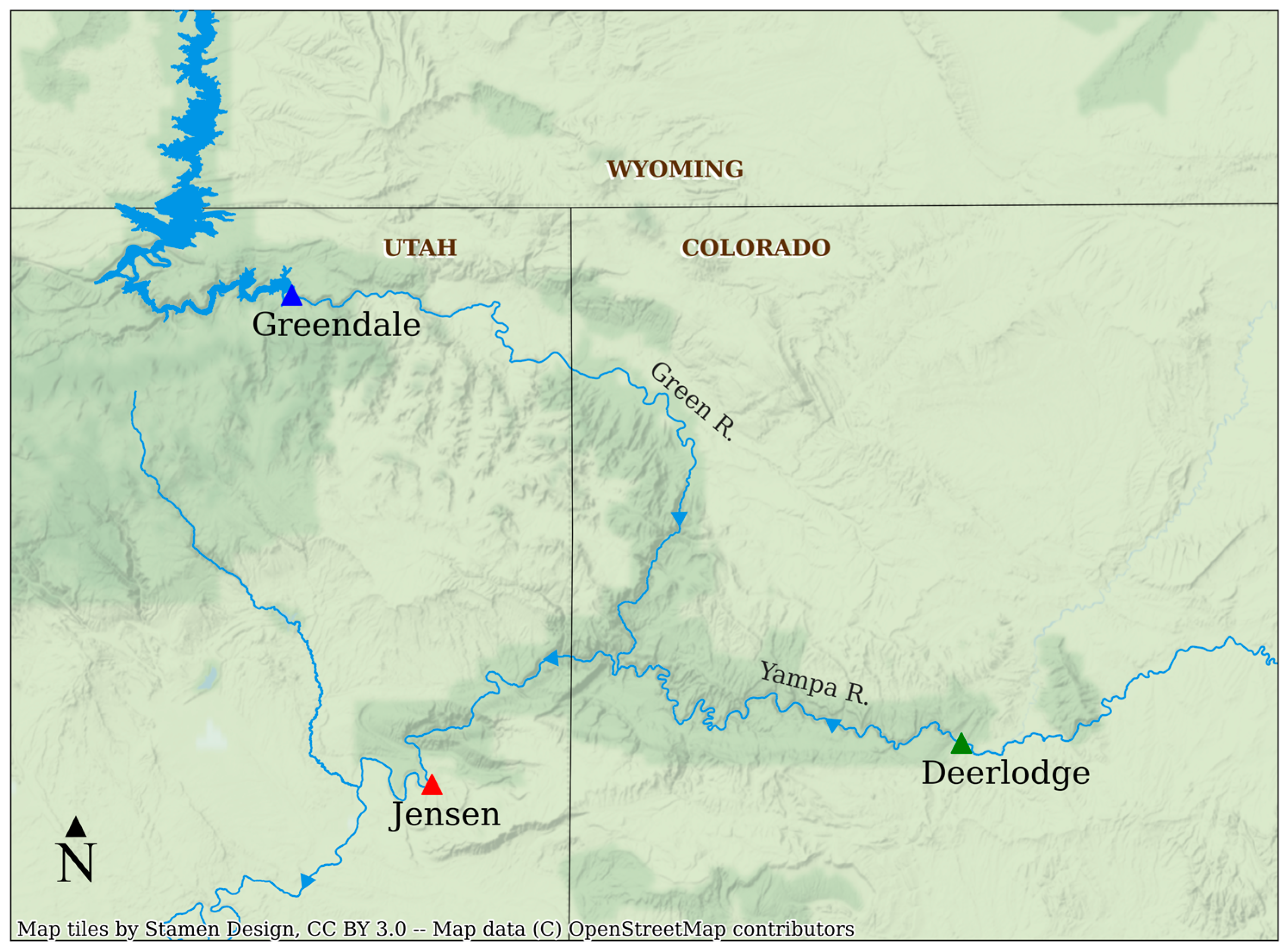
The site used to assess the performance of the proposed methods is the river system located on the Green River and Yampa River and delimited by the Flaming Gorge Dam (first upstream source), the Deerlodge Park gage (second upstream source), and the Jensen gage (downstream point) (see Figure 2).
The Green River is a major tributary of the Colorado River, flowing through Utah, Colorado, Wyoming and Arizona. The Flaming Gorge Dam impounds the Upper Green River, creating the 91-mile (~146-km) Flaming Gorge Reservoir, 400 miles (~643 km) upstream of the major Colorado and Green River confluence. Constructed from 1958 to 1964, the reservoir and dam play crucial roles in flood control, hydropower generation, irrigation, and recreation. The Yampa River is a major tributary of the Green River, flowing through northwestern Colorado. The Yampa River meets the Green River at the confluence near the Dinosaur National Monument in Colorado and Utah. The Jensen gage is a river gage located on the Green River near Jensen, Utah, 28.6 miles downstream of the Yampa confluence. The Jensen gage is used to measure the flow of the Green River and monitor its water levels.
Per the most recent Flaming Gorge Environmental Impact Statement (EIS) [39], during the base flow period (from mid-July to the end of February), hourly release patterns from the Flaming Gorge Dam must be not produce more than a 0.1 m stage change at the Jensen gage within a 24 h period, except during emergency operations. This restriction is part of a broader set of environmental regulations imposed on the Flaming Gorge Dam operations to achieve the flow and temperature regimes recommended by the Upper Colorado River Endangered Fish Recovery Program (Recovery Program) [40]. One of the goals of these environmental regulations is to protect critical nursery habitats for endangered fish in the Green River downstream from Jensen.
In order to comply with the 0.1 m stage change restriction at the Jensen gage, both BoR and WAPA have been relying on SSARR in their river simulation model and hydro-scheduling tool [41]. As seen above, SSARR includes a physics-based model designed to predict downstream river flow based on upstream discharges. In particular, SSARR is used by BoR and WAPA to predict Jensen flow rate based on Flaming Gorge Dam releases and Yampa flow rate. The Jensen stage level is then deduced from Jensen flow rate based on a flow-to-stage curve regularly updated by USGS [32]. However, the geometry and geology of the Green River and Yampa River have noticeably evolved since the first time SSARR was used to predict Jensen flow, in the 1990s. As a physics-based model, SSARR parameters require to be regularly updated by conducting detailed studies about the new river shape and soil conditions, which is not always feasible for economic reasons. As a result, the predictive ability of SSARR at the Jensen gage has been declining in the past decade.
By opposition, the LP and CNN models presented in this article are both empirical models and are designed to “learn”, i.e., automatically update, their predictive parameters based on the most recent hydrology time series data, which are publicly available and constantly monitored by USGS gages. The Green River system is used as a case study to assess the performance of both models and compare it to the performance of SSARR.

2.8. Datasets

Stream gage information is accessed via the National Water Information System using the instantaneous value data retrieval REST API [28]. The USGS uses a station number to categorize sites from which hydrological data are measured, included here as “USGS 0#######”. Flaming Gorge Dam release is approximated by the Green River near Greendale, UT stream gage (USGS 09234500); Yampa River by the gage at Deerlodge Park, UT (USGS 09260050); and Jensen by the Green River near Jensen, UT stream gage (USGS 09261000).

3. Results

Models are evaluated for two measures which serve specific considerations for 1D flow prediction for the Jensen, UT stream reach: prediction of (1) hourly flow, and (2) daily maximum stage change. Hourly flow prediction is the 1 h discharge series and performance demonstrates abilities of each model to forecast high-resolution 1D flow. Often, operational considerations may value flow summary metrics over hourly flow. The second measure used to compare model performance is important in the Jensen reach where daily maximum stage change is used for evaluating dam compliance with the 0.1 m stage requirement. Each measure is evaluated with four performance metrics: mean absolute error (MAE), mean squared error (MSE), coefficient of determination (R2), and the maximum error residual. Performance metrics are calculated on the test dataset.
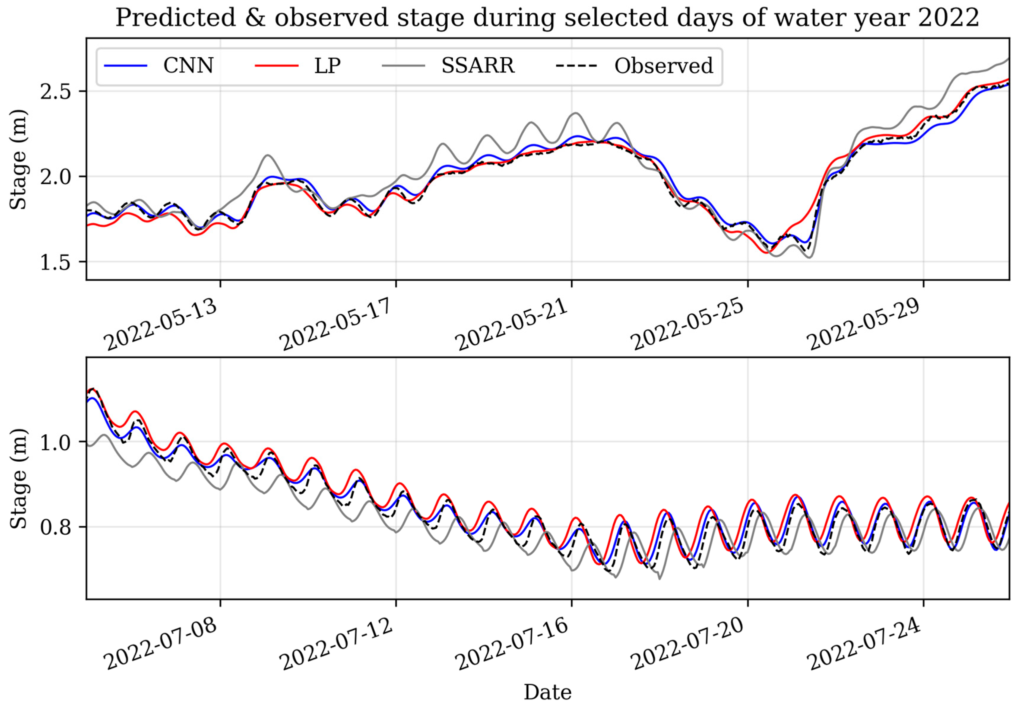
Flow predictions from SSARR, LP, and CNN were generated for water year 2022 (see example predictions in Figure 3) to compare the performance of each method. Table 1 shows training time and performance for both evaluation metrics across the two data-driven approaches (LP and CNN) compared to the SSARR hydrologic model. The data-driven LP and CNN models outperform SSARR under both hourly and daily min-to-max performance metrics. CNN has a mean absolute error approximately 42% smaller than LP for hourly flow, but mean squared error over 70% smaller, indicating a smaller number of larger errors in the hourly forecast. Despite performing better for hourly prediction, CNN and LP have relatively similar performance for the daily min-to-max measure. Notably, LP has a smaller maximum residual than CNN under the daily min-to-max measure. It is likely this discrepancy is due to chance rather than a structural difference that allows LP to out-perform CNN for daily min-to-max stage. The LP model can be computed about ten times faster than the CNN, but both models can be trained in under five minutes.
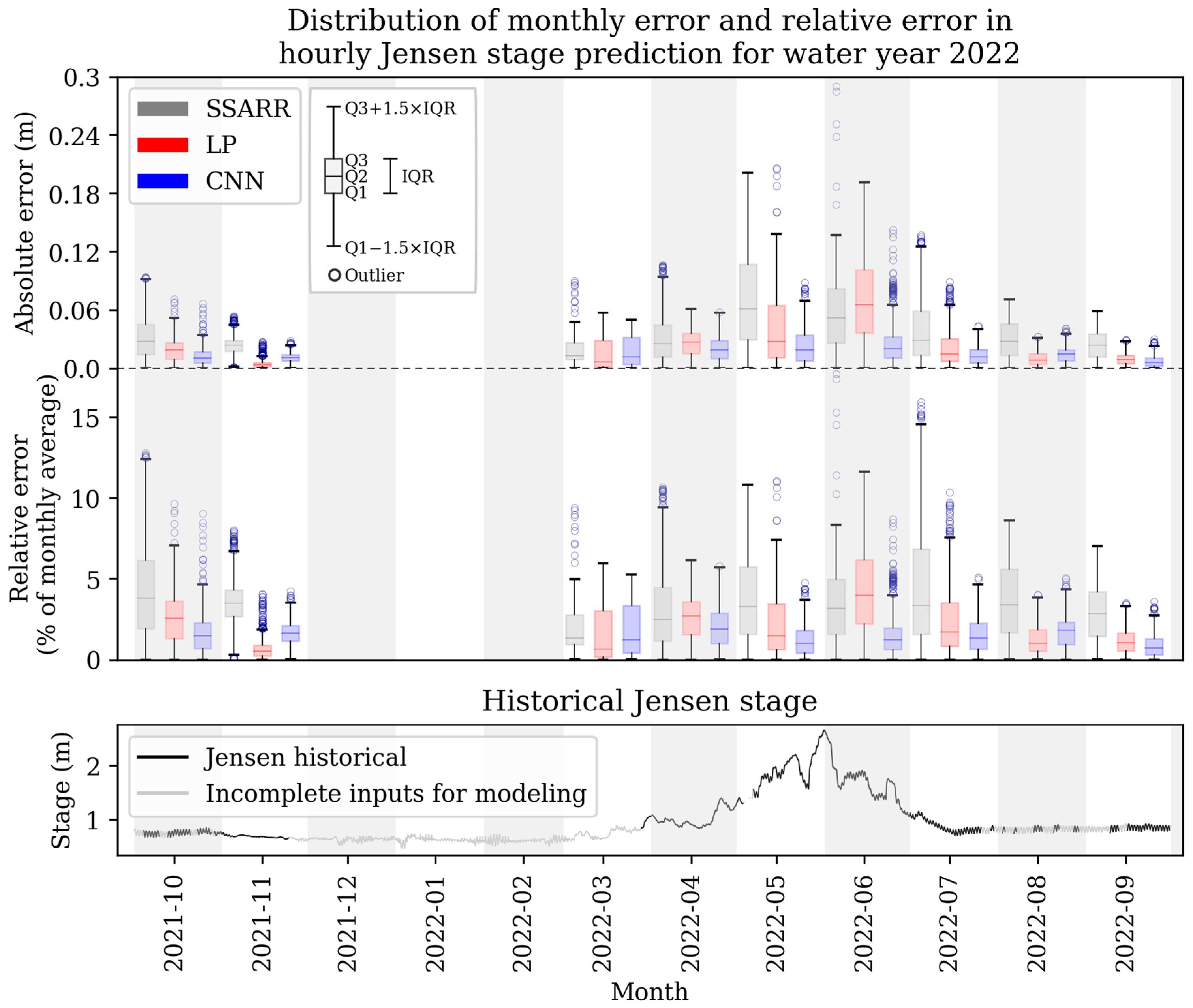
We are also interested in the performance of each stage model over the course of the model year and at different discharge magnitudes. Monthly error distributions from each model are shown in Figure 4. Due to large differences in flow magnitudes over the water year, the distribution of relative error (absolute error divided by monthly average stage) is also shown. While absolute error is higher when the stage near Jensen is larger, there is no evident pattern in relative error over the water year. Notably, during July through November, LP and CNN significantly outperform the SSARR model with smaller errors.
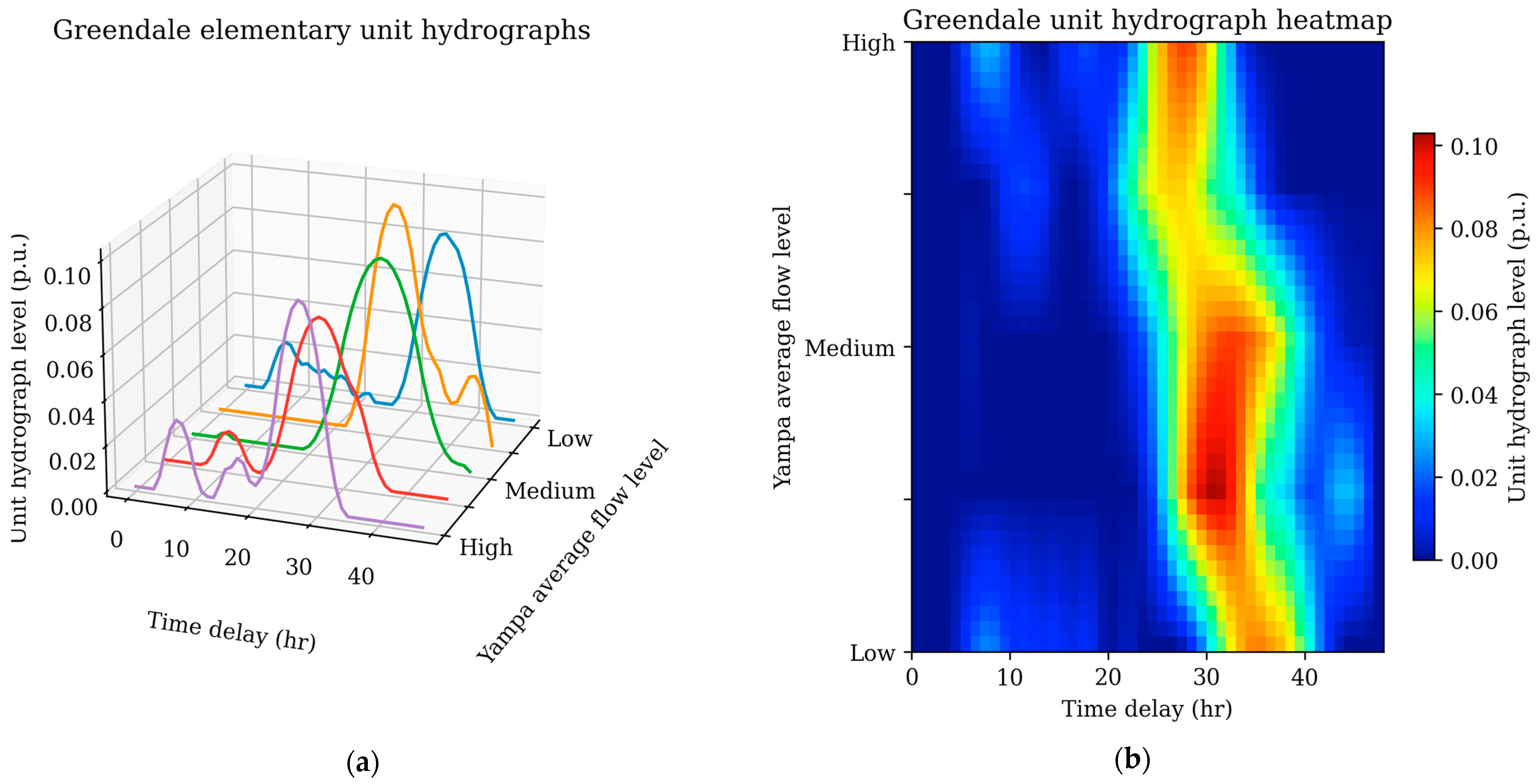
Both models are developed by applying convolution to upstream hydrographs to predict Jensen flow. LP is applied by considering Jensen flow as an evolving linear combination of five unit hydrographs for each of the two upstream sources. As described in the linear programming model section, the LP model is solved to learn the optimal unit hydrographs from the training set, and these optimal unit hydrographs are used to predict the downstream river discharge in the test set. The downstream river stage is then calculated using the Jensen flow-to-stage empirical function [32]. The input parameters a k , l , t describing the slowly evolving change in the unit hydrograph is based on the average monthly discharge at Yampa. Figure 5 below illustrates the five optimal unit hydrographs identified by the LP model for the Greendale upstream source (USGS 09234500). Note that the average time delay from Greendale to Jensen is decreasing as the average Yampa flow level increases. As Yampa flow speed increases, it increases flow speed on the Green River which reduces water travel time from Greendale.
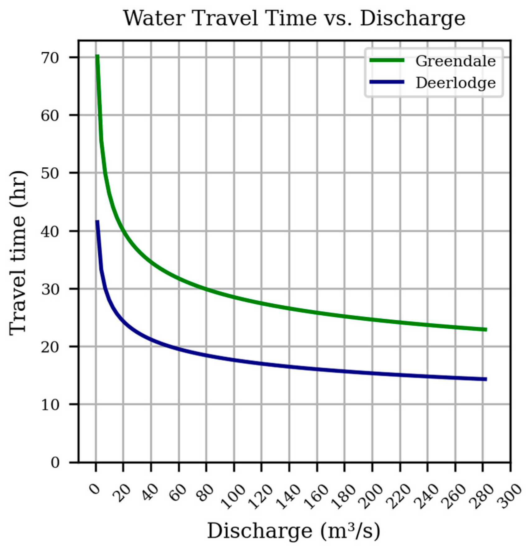
The CNN considers Jensen flow as a convolution of the two series produced when applying a discharge-variant lag to Greendale and Deerlodge hydrographs. The discharge-variant lag applied to upstream sources, modeled as an exponential function, would be analogous to the LP’s varying unit hydrographs at different flow magnitudes. To fit the exponential function, the maximum cross-correlation algorithm described in the Discharge-Variant Water Travel Time section is used to aggregate a sample dataset. Manual data cleansing is required to fit a clean exponential function. Figure 6 demonstrates the exponential function fit for one training fold. As expected, the water travel time increases as discharge decreases for both upstream sources.
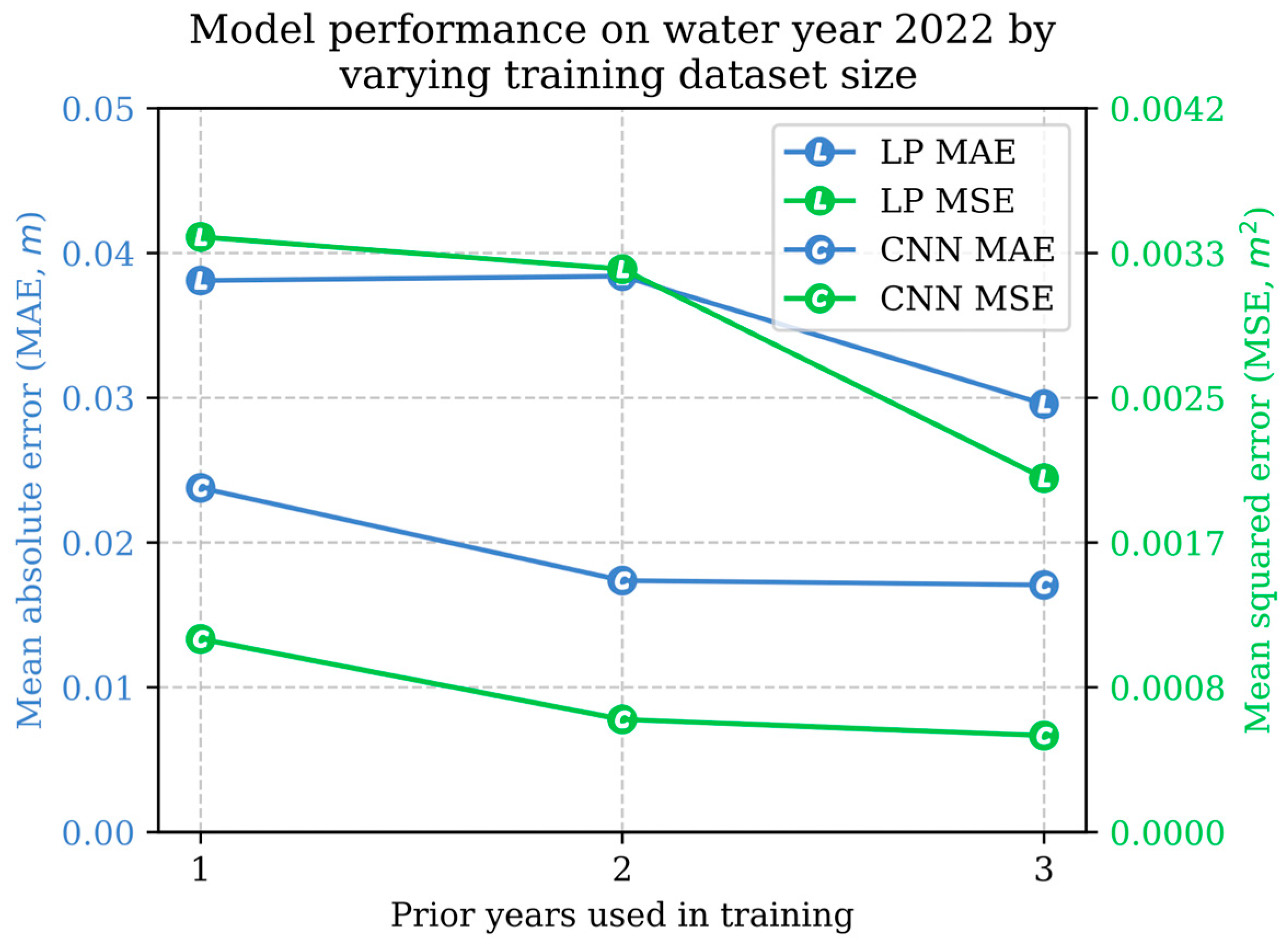
An important consideration for water managers and modelers using empirical techniques for 1D flow prediction is the training dataset size, which impacts the accuracy of the model. To examine the effect of training dataset size on accuracy, the LP and CNN models were trained by varying the training dataset length. Since water year 2022 is used as the evaluation dataset, training datasets with 1, 2, and 3 years of data prior to water year 2022 were used to train both models (the models trained on 3 years of data are the same models presented previously). The MAE and MSE from these experiments are shown for the LP and CNN models in Figure 7. Both CNN and LP models are impacted by training dataset length, though CNN impressively has very similar performance between models trained on 2 prior years and 3 prior years.

4. Discussion

The data-driven approaches used by the LP and CNN models demonstrate considerable prediction capabilities for addressing the challenge of 1D flow forecasting. Though modelers must consider a variety of stakeholder needs when considering methods for 1D flow, a major advantage of empirical modeling is the ability to quickly relearn hydrologic relationships at a low cost when model performance inevitably degrades. Indeed, contrary to physics-based models that require an accurate and thorough description of numerous watershed characteristics, including site geometry, and evolving soil moisture, infiltration, land use, and surface friction, the data-driven approaches presented here only require time series data from constantly monitoring and relatively low-cost gages. Because of this, the adoption of such data-driven approaches for river discharge and stage prediction has significant cost savings potential for future hydrology/hydropower-related studies.
Selecting a data-driven approach is another serious consideration. This manuscript introduces two viable solutions: a linear mathematical optimization (LP) model and one that uses artificial intelligence with non-linearities (CNN). Both models can learn optimal prediction parameters based on historical flow data and they both use convolution methods when predicting output results. We demonstrate that both models have similar performances when predicting downstream river stage at the Jensen gage. The CNN model demonstrates higher prediction accuracy than the LP model at an hourly resolution. However, the difference in prediction accuracy becomes negligeable when comparing daily min-to-max results. This implies that both models exhibit similar performances when predicting whether the water level at the Jensen gage complies with the environmental 0.1 m stage change restriction. The strength of the CNN model is based on its ability to explicitly model non-linearities between the discharge and stage data of the system, owing to its neural network structure. Contrary to the CNN model, the LP model is only able to model linear relationships, which limits its predictive ability to downstream discharge based on upstream discharges. To predict downstream stage, an additional step is required with the LP model, in which predicted discharge is converted to predicted stage owing to an empirical flow-to-stage function. This implies that its ability to predict downstream stage is limited by the accuracy of the flow-to-stage function. However, the strength of the LP model is based on its ability to identify linear predictive functions (i.e., the unit hydrographs) that are mathematically guaranteed to ensure the minimum possible prediction error. Moreover, powerful state-of-the-art LP solving methods such as the interior-point method [42] enable the optimal predictive functions to be identified in just a few seconds, even when considering time series of thousands of data points. The linear predictive functions identified by the LP model also make them more suitable to be integrated in linear water management tools or hydropower scheduling models such as GTMaxSL [27].
As demonstrated, the performance of empirical models also relies primarily on the quality of the observation data used to train them. While the LP and CNN models both perform with reasonable accuracy when decreasing the training dataset size, the performance degradation is significant when only using 1 year of data. It should also be expected that when river conditions (e.g., magnitude of flow, riverbed characteristics, or river geometry) deviate from the conditions represented by the training dataset, prediction accuracy will be hampered.
In summary, the structure of the CNN model and its explicit modeling of non-linearities makes it ideal to accurately predict downstream measures at a high time resolution (hours, minutes) that may include water discharge, water level, but also other environmental measures (e.g., temperature, gas concentration). On the other hand, the formulation of LP model and its ability to identify optimal linear predictive parameters makes it ideal to be integrated in linear water management tools or hydropower scheduling models.

5. Conclusions

This paper introduces two novel empirical models to predict downstream river flow and stage based on upstream flow data. Both models are based on convolution methods and are designed to learn predictive parameters using a training dataset (measured hydrologic data). The LP model solves a linear mathematical optimization problem to identify slowly evolving unit hydrographs that describe the impact of the upstream water flows on the downstream flow. The predicted downstream flow can later be translated into a river stage via an empirical flow-to-stage function. Conversely, the CNN model learns to directly predict the downstream stage based on upstream flows owing to a non-linear neural network. When tested on a real-world case study, both models show promising results and outperform the physics-based model currently used by federal agencies on the selected river system. Further work is needed to identify the ideal size of the training period, as there is a tradeoff between having a large enough training dataset and recent historical data. Alternatively, the prediction error of the hydrologic variables could be weighted based on how recent they are.

Author Contributions

Conceptualization, J.F., Q.P., T.V. and E.Y.; methodology, J.F., Q.P., T.V. and E.Y.; software, J.F. and Q.P.; validation, J.F. and Q.P.; formal analysis, J.F. and Q.P.; investigation, J.F. and Q.P.; resources, J.F., Q.P., T.V. and E.Y.; data curation, J.F. and Q.P.; writing—original draft preparation, J.F. and Q.P.; writing—review and editing, J.F. and Q.P.; visualization, J.F. and Q.P.; supervision, T.V., and E.Y.; project administration, T.V. and E.Y.; funding acquisition, J.F., Q.P., T.V. and E.Y. All authors have read and agreed to the published version of the manuscript.

Funding

Argonne National Laboratory’s work was supported by the Western Area Power Administration under interagency agreement through the U.S. Department of Energy contract DE-AC02-06CH11357.

Data Availability Statement

Data available from the USGS National Water Information System (NWIS) [28].

Acknowledgments

We gratefully acknowledge the computing resources provided on Swing and Bebop, high-performance computing clusters operated by the Laboratory Computing Resource Center at Argonne National Laboratory.

Conflicts of Interest

The authors declare no conflict of interest. The funders had no role in the design of the study; in the collection, analyses, or interpretation of data; in the writing of the manuscript; or in the decision to publish the results.

Appendix A

  • Detailed mathematical formulation of the LP method
(A1) M i n t = 0 T 1 δ t + c k = 1 K l = 1 L s k , l (A2) s . t .   Q t d Q t d ^ δ t t 0 , , T 1 (A3) Q t d Q t d ^ δ t t 0 , , T 1 (A4) Q t d ^ = k = 1 K Q k , t d ^ t 0 , , T 1 (A5) Q k , t d ^ = l = 1 L a k , l , t q k , l , t d t T H 1 , , T 1 , k 1 , , K (A6) q k , l , t d = h k , l , t Q k , t u = u = 0 T H 1 h k , l , u Q k , t u u t 0 , , T 1 , k 1 , , K , l 1 , , L (A7) M k , l = t = 0 T H 1 h k , l , t k 1 , , K , l 1 , , L (A8) M k , l M k , l ¯ k 1 , , K , l 1 , , L (A9) M k , l M k , l ¯ k 1 , , K , l 1 , , L (A10) h k , l , t = 0 t E k , l , k 1 , , K , l 1 , , L (A11) d k , l , t = h k , l , t + 1 2 h k , l , t + h k , l , t 1 t 1 , , T 2 , k 1 , , K , l 1 , , L (A12) d k , l , t s k , l t 1 , , T 2 , k 1 , , K , l 1 , , L (A13) d k , l , t s k , l t 1 , , T 2 , k 1 , , K , l 1 , , L
  • Sets
t 0 , , T 1 : time steps of the historical time series, with T being the length of the time series;
u 0 , , T H 1 : time steps of the unit hydrographs, with T H being the maximum length of the unit hydrographs and T H < T ;
k 1 , , K : index of the reach/upstream river source;
l 1 , , L : index of the elementary unit hydrograph for a given upstream river source;
E k , l : subset of time steps t for which the value of h k , l , t is constrained to be zero.
  • Parameters
Q t d : historical discharge (flow) level at the downstream river point in time step t .
Q k , t u : historical discharge (flow) level at the upstream river source k in time step t .
a k , l , t : “percentage” component of unit hydrograph index k , l in time step t . This coefficient is predefined by the user and verifies: l = 1 L a k , l , t = 1.0 for all k , t .
M k , l ¯ , M k , l ¯ : lower and upper bounds of the mass balance indicator of unit hydrograph index k , l .
c : smoothness coefficient; the larger its value, the smoother the unit hydrograph.
  • Variables
Q t d ^ : estimator of the discharge (flow) level at the downstream river point in time step t ;
δ t : absolute difference between the historical value and the estimated value of the discharge (flow) level at the downstream river point in time step t ;
Q k , t d ^ : component of the downstream discharge estimator related to upstream river source k in time step t ;
q k , l , t d : component of the downstream discharge estimator related to upstream river source k and unit hydrograph index l in time step t ;
h k , l , t : value of the unit hydrograph index l of upstream river source k in time step t ;
d k , l , t : discrete second order derivative of variable h k , l , t ;
s k , l : upper bound on the absolute value of the discrete second order derivative d k , l , t ;
M k , l : mass balance indicator associated to unit hydrograph index l at upstream river source k .
  • Description
Equation (A1) is the objective function and simultaneously minimizes the estimation error of the predicted downstream flow and the variability of the unit hydrographs. More specifically, Equation (A1) concurrently minimizes (a) the sum of absolute differences between the downstream flow estimator and its historical value, and (b) the sum of maximum absolute value of the second order derivative of each unit hydrograph. The first component is introduced to minimize the error in approximating the downstream flow, whereas the second component is introduced to increase the smoothness of the unit hydrographs. Real-world unit hydrographs are expected to be relatively smooth. However, measured discharge data are imperfect and inevitably introduce some noise in the model. As a result, without the smoothness component in the objective function, the optimal unit hydrographs identified by the LP model would exhibit unrealistic noise. A small enough smoothness coefficient c guarantees to identify smooth unit hydrographs with little impact on the estimation error. Equations (A2) and (A3) define δ t as an upper bound of the error in approximating the downstream flow in time t. More specifically, the minimization of δ t by Equation (A1) guarantees that the optimal value of δ t is exactly equal to the absolute difference between historical and estimator value in time t. Equation (A4) defines the downstream flow estimator as the sum of the individual upstream components. Equation (A5) allows each upstream component Q k , t d ^ of the downstream flow estimator to be defined as an evolving linear combination of subcomponents q k , l , t d . Each subcomponent q k , l , t d is defined as the convolution between the historical upstream flow Q k , t u and an elementary unit hydrograph h k , l , t , as described in Equation (A6). The coefficients a k , l , t of the evolving linear combination are predefined by the user and can be based on the time of the year, weather conditions, or hydrology conditions. Equation (A7) defines the mass balance indicators M k , l as the integral of the unit hydrographs. This mass balance indicator represents the percentage of water volume from an upstream source that will eventually reach the downstream point. Ideally, this percentage should be equal to 100% but diverse phenomena such as soil absorption or small, unaccounted, river tributaries may either decrease or increase this value. Equations (A8) and (A9) allow the user to restrict the value of the mass balance indicator between predefined bounds. Additionally, Equation (A10) allows the user to impose the value of the unit hydrograph to be zero in predefined ranges E k , l . For example, imposing the value of the unit hydrograph h k , l , t to be zero in time steps t 0 , , 7 will inform the model that the discharge from the upstream source k cannot take less than 8 h to reach the downstream point. Equation (A11) defines d k , l , t as the discrete second order derivative of the unit hydrographs. Equations (A12) and (A13), together with the minimization imposed by Equation (A1), ensure that the maximum absolute value of d k , l , t is as low as possible. Minimizing the maximum absolute value of the second order derivative of a unit hydrograph is equivalent to maximizing the unit hydrograph smoothness. Indeed, the smoothness of a time series can be defined as the rate of change or slope of the time series at different points in time. A time series with a consistently low rate of change is typically considered smoother than a series with a high rate of change.
  • Unit hydrograph and link to water travel time and mass balance indicator
The unit hydrograph h k , l , t of a river reach between an upstream source k and a downstream point is also known as the water travel time distribution (WTTD) on that river reach. Concretely, h k , l , t represents the portion of a volume of water discharged at the upstream source k that will reach the downstream point after a certain time delay t . As a result, h k , l , t can be thought as the probability density function (PDF) for a volume of water to have a travel time t through the reach. However, the integral of a PDF must be equal to 1, which is not necessarily the case of h k , t . Indeed, as seen above, diverse physics phenomena prevent the mass balance indicator M k , l = t = 0 T H 1 h k , l , t from being exactly equal to 1. Instead, the rescaled unit hydrograph h k , l , t = h k , l , t / M k , l verifies this necessary condition. It follows that the average water travel time t k , l u d in reach k can be calculated as
t k , l u d = t = 0 T H h k , l , t · t d t = t = 0 T H 1 h k , l , t · t = t = 0 T H 1 h k , l , t · t M k , l
Additionally, the mass balance indicator M k , l = t = 0 T H 1 h k , l , t represents the total portion of water discharged at the upstream source k that eventually reaches the downstream river point. As explained above, ideally, this quantity should be equal to 1. However, a portion of the water traveling through the reach may end up being absorbed in the soil or evaporated, thus decreasing the value of M k , l . Conversely, rain or water inflows from small, unaccounted, river tributaries may increase the value of M k , l . As a result, it is not realistic to expect the value of M k , l to be equal to 1. This is why, instead of being constrained equal to 1, the value of M k , l is bounded (Equations (A8) and (A9)). However, the phenomena described above are assumed to have a relatively low impact and, in practice, the value of the bounds M k , l ¯ and M k , l ¯ can be set equal to 0.9 and 1.1, respectively.

Appendix B

Table A1. Search space for Bayesian optimization and optimal values of CNN hyperparameters. Number of convolutional layers refers to the number of stacked convolution operations in the CNN, represented as L in Equation (11); number of convolution filters refers to the number of independent convolution designs in each convolution layer, represented as C in Equation (11); kernel size is the number of contiguous timesteps used in a convolution, represented as the length of vector w in Equation (11); kernel non-negative constraint refers to a numerical constraint added to the convolution filters; kernel regularizer L2 factor is L2 regularization factor applied to the kernel weights during training; learning rate is used to adjust the relative effect of model loss on parameter updates after each training epoch; and batch size is the number of data points used in one training step. Type indicates whether the variable has discrete types (e.g., “discrete” and “Boolean”) or can occupy a range of values (e.g., “continuous”). Domain defines the numerical space to search.
ParameterTypeDomainOptimized ValueNote
Number of convolution layersDiscrete(1, 10)5
Number of convolution filtersDiscrete{4, 8, 16, 32, 64}16
Kernel sizeDiscrete(4, 193) 24Subject to number of convolutions
Kernel non-negative constraintBoolean{True, False}False
Kernel regularizer L2 factor Continuous(0, 0.1)0.03
Learning rateContinuous(0.00001, 0.01)0.002
Batch sizeDiscrete{64, 128, 256}64

References

  1. Worster, D. Rivers of Empire: Water, Aridity, and the Growth of the American West; Oxford University Press: Oxford, UK, 1992; ISBN 978-0-19-507806-0. [Google Scholar]
  2. Allan, C.; Xia, J.; Pahl-Wostl, C. Climate Change and Water Security: Challenges for Adaptive Water Management. Curr. Opin. Environ. Sustain. 2013, 5, 625–632. [Google Scholar] [CrossRef]
  3. Nanditha, J.S.; Mishra, V. On the Need of Ensemble Flood Forecast in India. Water Secur. 2021, 12, 100086. [Google Scholar] [CrossRef]
  4. Cueto-Felgueroso, L.; Santillán, D.; García-Palacios, J.H.; Garrote, L. Comparison between 2D Shallow-Water Simulations and Energy-Momentum Computations for Transcritical Flow Past Channel Contractions. Water 2019, 11, 1476. [Google Scholar] [CrossRef]
  5. Box, G.E.P.; Jenkins, G.M.; Reinsel, G.C. Linear Stationary Models. In Time Series Analysis; John Wiley & Sons, Ltd.: Hoboken, NJ, USA, 2008; pp. 47–91. ISBN 978-1-118-61919-3. [Google Scholar]
  6. Cryer, J.D.; Chan, K.-S. Time Series Analysis; Springer Texts in Statistics; Springer: New York, NY, USA, 2008; ISBN 978-0-387-75958-6. [Google Scholar]
  7. Salas, J.D.; Delleur, J.W.; Yevjevich, V.; Lane, W.L. Applied Modeling of Hydrologic Time Series; Water Resources Publications: Littleton, CO, USA, 1980; ISBN 978-0-918334-37-4. [Google Scholar]
  8. Bisgaard, S.; Kulahci, M. Time Series Analysis and Forecasting by Example; Wiley Series in Probability and Statistics; Wiley: Hoboken, NJ, USA, 2011; ISBN 978-0-470-54064-0. [Google Scholar]
  9. Pekarova, P.; Pekar, J. Long-Term Discharge Prediction for the Turnu Severin Station (the Danube) Using a Linear Autoregressive Model. Hydrol. Process. 2006, 20, 1217–1228. [Google Scholar] [CrossRef]
  10. Beyaztas, U.; Shang, H.L.; Yaseen, Z.M. A Functional Autoregressive Model Based on Exogenous Hydrometeorological Variables for River Flow Prediction. J. Hydrol. 2021, 598, 126380. [Google Scholar] [CrossRef]
  11. Abrahart, R.J.; See, L. Comparing Neural Network and Autoregressive Moving Average Techniques for the Provision of Continuous River Flow Forecasts in Two Contrasting Catchments. Hydrol. Process. 2000, 14, 2157–2172. [Google Scholar] [CrossRef]
  12. Anderson, P.L.; Meerschaert, M.M.; Zhang, K. Forecasting with Prediction Intervals for Periodic Autoregressive Moving Average Models. J. Time Ser. Anal. 2013, 34, 187–193. [Google Scholar] [CrossRef]
  13. Mohammadi, K.; Eslami, H.R.; Kahawita, R. Parameter Estimation of an ARMA Model for River Flow Forecasting Using Goal Programming. J. Hydrol. 2006, 331, 293–299. [Google Scholar] [CrossRef]
  14. Fashae, O.A.; Olusola, A.O.; Ndubuisi, I.; Udomboso, C.G. Comparing ANN and ARIMA Model in Predicting the Discharge of River Opeki from 2010 to 2020. River Res. Appl. 2019, 35, 169–177. [Google Scholar] [CrossRef]
  15. Lin, J.-Y.; Cheng, C.-T.; Chau, K.-W. Using Support Vector Machines for Long-Term Discharge Prediction. Hydrol. Sci. J. 2006, 51, 599–612. [Google Scholar] [CrossRef]
  16. Ghorbani, M.A.; Zadeh, H.A.; Isazadeh, M.; Terzi, O. A Comparative Study of Artificial Neural Network (MLP, RBF) and Support Vector Machine Models for River Flow Prediction. Environ. Earth Sci. 2016, 75, 476. [Google Scholar] [CrossRef]
  17. Kişi, Ö. River Flow Modeling Using Artificial Neural Networks. J. Hydrol. Eng. 2004, 9, 60–63. [Google Scholar] [CrossRef]
  18. Chang, F.-J.; Chen, P.-A.; Lu, Y.-R.; Huang, E.; Chang, K.-Y. Real-Time Multi-Step-Ahead Water Level Forecasting by Recurrent Neural Networks for Urban Flood Control. J. Hydrol. 2014, 517, 836–846. [Google Scholar] [CrossRef]
  19. Tian, Y.; Xu, Y.-P.; Yang, Z.; Wang, G.; Zhu, Q. Integration of a Parsimonious Hydrological Model with Recurrent Neural Networks for Improved Streamflow Forecasting. Water 2018, 10, 1655. [Google Scholar] [CrossRef]
  20. Vieux, B.E.; Cui, Z.; Gaur, A. Evaluation of a Physics-Based Distributed Hydrologic Model for Flood Forecasting. J. Hydrol. 2004, 298, 155–177. [Google Scholar] [CrossRef]
  21. Butler, T.; Graham, L.; Estep, D.; Dawson, C.; Westerink, J.J. Definition and Solution of a Stochastic Inverse Problem for the Manning’s n Parameter Field in Hydrodynamic Models. Adv. Water Resour. 2015, 78, 60–79. [Google Scholar] [CrossRef]
  22. Yang, D.Y.; Frangopol, D.M. Physics-Based Assessment of Climate Change Impact on Long-Term Regional Bridge Scour Risk Using Hydrologic Modeling: Application to Lehigh River Watershed. J. Bridg. Eng. 2019, 24, 04019099. [Google Scholar] [CrossRef]
  23. Hussain, F.; Wu, R.-S.; Wang, J.-X. Comparative Study of Very Short-Term Flood Forecasting Using Physics-Based Numerical Model and Data-Driven Prediction Model. Nat. Hazards 2021, 107, 249–284. [Google Scholar] [CrossRef]
  24. Sepúlveda, U.M.; Mendoza, P.A.; Mizukami, N.; Newman, A.J. Revisiting Parameter Sensitivities in the Variable Infiltration Capacity Model across a Hydroclimatic Gradient. Hydrol. Earth Syst. Sci. 2022, 26, 3419–3445. [Google Scholar] [CrossRef]
  25. United States Army Corps of Engineers North Pacific Division. Program Description and User Manual for SSARR, Streamflow Synthesis and Reservoir Regulation: Program 724-K5-G0010; Army Engineer Division, North Pacific: Honolulu, HI, USA, 1975.
  26. Zagona, E.A.; Fulp, T.J.; Shane, R.; Magee, T.; Goranflo, H.M. Riverware: A Generalized Tool for Complex Reservoir System Modeling1. JAWRA J. Am. Water Resour. Assoc. 2001, 37, 913–929. [Google Scholar] [CrossRef]
  27. Ploussard, Q.; Veselka, T.D.; Palmer, C.S. Economic Analysis of Changes in Hydropower Operations at the Flaming Gorge Dam and the Aspinall Unit Due to the Upper Colorado River Endangered Fish Recovery Program; Argonne National Lab. (ANL): Argonne, IL, USA, 2022.
  28. U.S. Geological Survey. USGS Water Data for the Nation; U.S. Geological Survey: Reston, VA, USA, 1994. [CrossRef]
  29. Nash, J.E. Systematic Determination of Unit Hydrograph Parameters. J. Geophys. Res. 1959, 64, 111–115. [Google Scholar] [CrossRef]
  30. Boyd, S.; Vandenberghe, L. Convex Optimization; Cambridge University Press: Cambridge, UK, 2004. [Google Scholar]
  31. Zhao, B.; Tung, Y.-K. Determination of Optimal Unit Hydrographs by Linear Programming. Water Resour. Manag. 1994, 8, 101–119. [Google Scholar] [CrossRef]
  32. Sauer, V.B. Standards for the Analysis and Processing of Surface-Water Data and Information Using Electronic Methods; Water-Resources Investigations Report; U.S. Geological Survey: Reston, VA, USA, 2002; Volume 2001–4044.
  33. Gurobi Optimization, LLC. Gurobi Optimization Reference Manual; Gurobi Optimization, LLC: Beaverton, OR, USA, 2023. [Google Scholar]
  34. Kiranyaz, S.; Avci, O.; Abdeljaber, O.; Ince, T.; Gabbouj, M.; Inman, D.J. 1D Convolutional Neural Networks and Applications: A Survey. Mech. Syst. Signal Process. 2021, 151, 107398. [Google Scholar] [CrossRef]
  35. Abadi, M.; Agarwal, A.; Barham, P.; Brevdo, E.; Chen, Z.; Citro, C.; Corrado, G.S.; Davis, A.; Dean, J.; Devin, M.; et al. TensorFlow: Large-Scale Machine Learning on Heterogeneous Distributed Systems. arXiv 2016, arXiv:1603.04467. [Google Scholar]
  36. The GPyOpt Authors. GPyOpt: A Bayesian Optimization Framework in Python 2016. Available online: http://github.com/SheffieldML/GPyOpt (accessed on 8 October 2023).
  37. Kingma, D.P.; Ba, J. Adam: A Method for Stochastic Optimization. arXiv 2017, arXiv:1412.6980. [Google Scholar]
  38. Grippo, M.; LaGory, K.E.; David, W.; Hayse, J.W.; Walston, L.J.; Weber, C.C.; Magnusson, A.K.; Jiang, X.H. Relationships between Flow and the Physical Characteristics of Colorado Pikeminnow Backwater Nursery Habitats in the Middle Green River, Utah; Final Report to Upper Colorado River Endangered Fish Recovery Program; Argonne National Laboratory: Lemont, IL, USA, 2017.
  39. U.S. Bureau of Reclamation. Record of Decision: Operation of Flaming Gorge Dam Final Environmental Impact Statement; U.S. Bureau of Reclamation: Washington, DC, USA, 2006.
  40. Muth, R.T.; Crist, L.W.; LaGory, K.E.; Hayse, J.W.; Bestgen, K.R.; Ryan, T.P.; Lyons, J.K.; Valdez, R.A. Flow and Temperature Recommendations for Endangered Fishes in the Green River Downstream of Flaming Gorge Dam; Final Report FG-53 to the Upper Colorado River Endangered Fish Recovery Program; Larval Fish Laboratory Contribution 120; U. S. Fish and Wildlife Service: Denver, CO, USA, 2000.
  41. Yin, S.C.L.; Tomasko, D.; Cho, H.E.; Williams, G.; McCoy, J.; Palmer, C. Effects of Flaming Gorge Dam Hydropower Operations on Downstream Flow, Stage, and Sediment Transport; Argonne National Lab. (ANL): Argonne, IL, USA, 1996.
  42. Potra, F.A.; Wright, S.J. Interior-Point Methods. J. Comput. Appl. Math. 2000, 124, 281–302. [Google Scholar] [CrossRef]
Figure 1. Daily averages for response (Jensen stage) and explanatory timeseries (Greendale and Deerlodge discharge) over the four water years used for modeling. The test split is shown as a dotted line at the start of the 2022 water year (1 October 2021). The cross-validation splits are shown as lighter dotted lines throughout the preceding three water years.
Water 15 03843 g001
Figure 2. Area of interest showing the Middle Green River system below the Flaming Gorge Dam. The Yampa River, a major gauged tributary recorded by the USGS gage in Deerlodge Park, CO (green), flows into the Green River. The Green River is gauged before and after the Yampa River inflow near Greendale, UT (blue) and Jensen, UT (red). The gage near Greendale, UT approximates flow releases at Flaming Gorge Dam. Dam release constraints established by the Flaming Gorge EIS are evaluated by flows measured at the gage near Jensen, UT. Arrows on river reaches indicate the direction of water flow.
Water 15 03843 g002
Figure 3. Hourly prediction and gage measurements for Jensen stage during selected periods of water year 2022 (top: 9–30 May 2022; bottom: 4–25 July 2022).
Water 15 03843 g003
Figure 4. Monthly distributions of hourly errors for each model (SSARR, LP, and CNN) over the test water year. Absolute error and relative error are shown. Relative error normalizes error magnitudes by discharge magnitude and is calculated as absolute error divided by the monthly average stage. Boxes extend from the first quartile (Q1) of error to the third quartile (Q3) of error with error medians (Q2) shown as divider line. The interquartile range (IQR) is defined as Q3−Q1. Whiskers show the 1.5 × IQR deviation from the first and third quartiles. Errors outside the 1.5 × IQR are shown as circles and may be considered outliers. The Jensen stage hydrograph, plotted below monthly error distributions, shows how flow varies throughout the year. During times throughout the water year (indicated by a gray Jensen stage hydrograph), full modeling inputs are not available for either SSARR, LP, or CNN due to sampling resolution or otherwise incomplete records.
Water 15 03843 g004
Figure 5. Illustration of the optimal unit hydrographs identified by the LP model for the Greendale upstream source. (a) Five elementary unit hydrographs h k , l , t . (b) Linear interpolation of these unit hydrographs. The LP model assumes that the unit hydrograph used to predict the downstream discharge level at a specific point in time is a linear interpolation of the elementary unit hydrographs based on the average Yampa flow level in that point in time.
Water 15 03843 g005
Figure 6. Water travel time curves between upstream sources (Greendale and Deerlodge) and the downstream Jensen gage.
Water 15 03843 g006
Figure 7. LP and CNN performance on the testing dataset (water year 2022) by varying the number of years preceding water year 2022 used for training. MAE and MSE are shown.
Water 15 03843 g007
Table 1. Time to train and performance metrics for hourly flow and daily minimum-to-maximum flow predicted by SSARR, LP, and CNN. The best performing metric is indicated in bold. Performance metrics for hourly flow and daily minimum-to-maximum flow include: mean absolute error (MAE) in m, mean squared error (MSE) in m2, coefficient of determination (R2) on a scale of 0 to 1, and the maximum error residual (m). The LP model is trained on laptop Intel Core i7-11800H with 32 GB of RAM; The CNN model is trained on a server NVIDIA A100 40 GB. Training time is the number of seconds it takes to train one complete CNN or LP model.
Training Time (Seconds)Hourly PredictionDaily Minimum-to-Maximum Prediction
Model MAE (m)MSE (m2)R2Max Error
Residual (m)
MAE (m)MSE (m2)R2Max Error
Residual (m)
SSARR-0.04110.00300.9870.2950.0270.00140.6690.180
LP170.02960.00200.9910.2100.0160.000560.8560.130
CNN1700.01710.000560.9980.1450.0150.000460.8770.142
Disclaimer/Publisher’s Note: The statements, opinions and data contained in all publications are solely those of the individual author(s) and contributor(s) and not of MDPI and/or the editor(s). MDPI and/or the editor(s) disclaim responsibility for any injury to people or property resulting from any ideas, methods, instructions or products referred to in the content.