1. Introduction
In Taiwan, aquaculture is an important economic pillar with an annual output value of over TWD 20 billion. However, traditional aquaculture is facing challenges such as an aging labor force, a lack of young workers, and the difficulty of transferring fishing knowledge to the next generation. Traditional aquaculture methods are labor-intensive and not cost-effective, leading to a transition toward smart aquaculture models with the rapid advancement of technology.
Based on the experiences of the older generation of fishermen, it is known that the length of the water-wheel tail is closely related to water quality. However, there is currently no systematic method to determine water quality, and adjustments are made based on visual inspection, relying heavily on experience without substantial data for transmission. This mode of judgment is difficult to fully pass on to the next generation. Furthermore, most water quality detection instruments available on the market are expensive and unaffordable for many aquaculture farmers. Sensors left in the water for an extended period are prone to interference from algae, leading to distorted data. Sending samples to county inspection centers for testing is time-consuming and not economically viable. Therefore, the primary challenge in aquaculture is how to effectively manage fish ponds, improve decision-making accuracy, reduce costs, and increase profits.
However, to achieve the above objectives, we believe that smart aquaculture will be an excellent approach. For example, Li et al. designed and implemented a system with multiple-parameter sensors, enabling aquaculture environment water quality monitoring, data collection, and analysis [
1]. This system assists fishermen in making aquaculture decisions and improves the level of aquaculture intelligence. Yuan et al. developed a water quality monitoring system that uses computer image processing technology to analyze fish behavior in real-time, thereby monitoring potential water contamination [
2]. Kassem et al. also created a smart aquaculture farm system that integrates recirculating aquaculture systems (RASs) and zero-water (ZWD) or discharge biological flocculation technology, incorporating monitoring and automation to ensure good water quality and high survival rates of aquatic life [
3]. By combining the information above, we designed a system based on fishermen’s wisdom, integrating monocular vision technology to effectively manage fish ponds and enhance decision-making accuracy.
Through the visual assessment method relied upon by fishermen, the quality of the fish and shrimps’ living environment and the trend of the length of foam trails generated by a water-wheel are determined to be related. When water-wheels are in operation, they produce foam, which is a phenomenon formed through the combination of soluble proteins and air in the water. The generation of foam can be influenced by various factors from different sources. Oh explored the relationship between the design of the condenser outlet of a thermal power plant and foam production, mentioning that high-temperature cooling water can promote algae growth, increase the amount of organic matter, and thereby increase the likelihood of foam formation [
4]. Jenkinson discussed the relationship between waves, ripples, foam, and aquatic organisms, stating that foam can regulate the exchange of air and substances in water, including greenhouse gases [
5]. Excessive and persistent foam generated by the water-wheel operation indicates a high organic matter content in the water [
6,
7]. Therefore, performing appropriate water exchange and reasonable feeding can reduce the concentration of organic matter [
8,
9].
When recording images of water-wheel trail with a camera, perspective distortion can occur due to factors such as shooting position and angle. Therefore, image projective transformation is needed to correct the images. Image projective transformation is used to correct camera lens distortion, enabling a more accurate image capture and the restoration of images to their original shapes, accounting for translation, rotation, or deformation, among other factors [
10,
11,
12]. For example, Chong et al. used image projective transformation to correct chest X-ray images captured with smartphones to improve the quality and discernibility of X-ray images [
13].
Multiple studies have shown that neural networks play a crucial role in object recognition [
14,
15,
16]. Their ability to automatically learn features, identify complex patterns, and adapt to new situations efficiently enables them to effectively distinguish object categories and continually improve recognition accuracy. For example, Yandouzi et al. combined deep learning object recognition with drone technology to detect fires and smoke in forests using YOLO v8, aiming to monitor forest fires [
17].
Data augmentation is a widely used technique in deep learning aimed at increasing the diversity of training data and improving model generalization [
18,
19,
20]. By applying random transformations or specific operations to training data, additional training samples are generated, enhancing data diversity [
21,
22,
23,
24]. In DeVries et al.’s research [
25], a data augmentation method called “Cutout” was proposed, which simulates image occlusion or missing parts by randomly blocking certain areas of the image to enhance the model’s ability to learn local details. Cubuk et al.’s study [
26] introduced a method named “AutoAugment”, which uses reinforcement learning algorithms to automatically learn suitable data augmentation strategies to enhance image classification performance. In the context of face recognition, Zhang et al.’s research [
27] presented a method called “Facial landmark-guided augmentation”, which adds virtual facial landmarks to facial images to increase the diversity of training samples.
Therefore, to address the challenge, a precise and efficient water quality control system is proposed in this study. This study aims to use photography to capture the water-wheel tail and perform image calibration and projective transformation on the photos using calibration boards. By utilizing known conditions and the proportional relationship, the actual length of the water-wheel tail can be calculated. Additionally, a target detection algorithm is employed to identify the characteristic of the water-wheel tail. The system’s key feature lies in its ability to measure and record the length of the water-wheel tail. In the future, the system’s measurement results will be combined with data from water-quality sensors. Through machine learning, the correlation between the two can be determined. Guo et al. utilized comprehensive data on early-season rice in China from 1981 to 2010, including phenological, climatic, pre-season, geographical, and yield data. They applied three advanced machine learning methods, namely, backpropagation neural network (BP), support vector machine (SVM), and random forest (RF), along with a traditional statistical approach, multiple linear regression (MLR), to model rice yield. This approach was employed to address the impact of phenology on rice yield prediction and to assess the influence of pre-season crops on rice yield prediction [
28]. Andrej et al. also employed automated machine learning to establish the knowledge base of an expert system for habitat suitability identification, specifically to determine the habitat range of brown bears in southwestern Slovenia [
29]. Similarly, Pham et al. used machine learning integration techniques to evaluate and compare landslide model performance for landslide susceptibility assessment [
30]. The information provided underscores the capacity of machine learning to assist in prediction, particularly in forecasting water quality changes based on water-wheel tail length trends [
31].
2. Materials and Methods
This study recorded the water-wheel tail using commercial cameras. The fish farms are located in Annan District, a coastal district located in the west of Tainan, Taiwan [
32], as shown in
Figure 1. Milkfish and white shrimp are mixed in the fish farms.
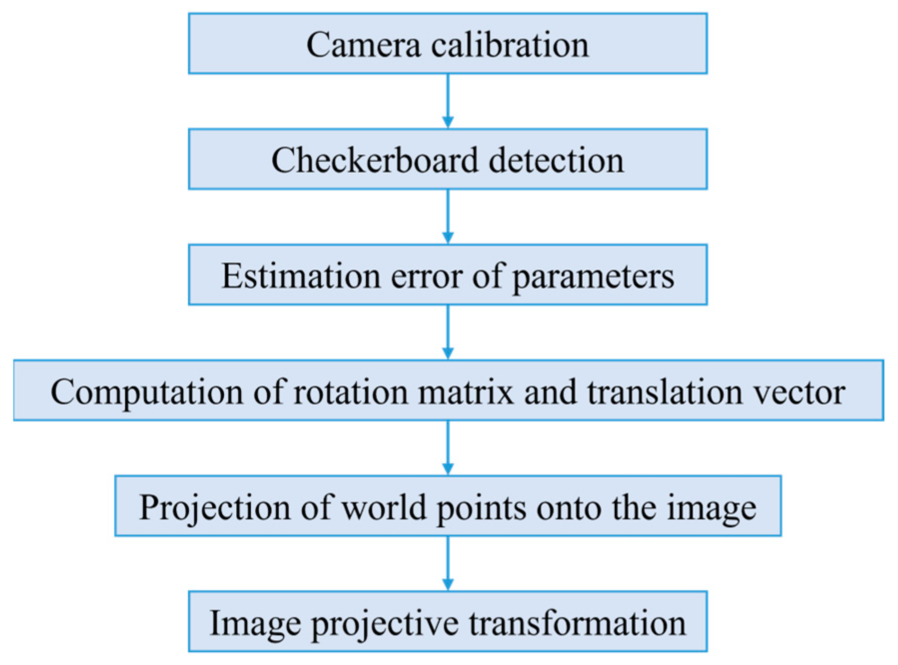
The purpose of this study is to measure the length of water-wheel tails through imagery. To achieve this, projective transformation is employed to obtain no-perspective-distortion images. Projective transformation is a type of transformation commonly used in geometry that maps one two-dimensional or three-dimensional space to another two-dimensional or three-dimensional space while preserving the collinearity of the points. Projection transformation can describe the projection process of a camera and eliminate the perspective distortion of an image. It is widely used in computer graphics, computer vision, and geometry. Suppose that the point of a point
transformed by projection is
, the relation can be expressed as:
where
and
are not zero, and
while
.
Figure 2 illustrates the schematic diagram of the projective transformation process, and it can be observed that the transformed image has been corrected to eliminate distortion. The definition of a water-wheel tail length is depicted in
Figure 3.
The definition of the water-wheel tail’s starting and ending points is based on the knowledge gained from fishermen’s experience. The starting point is the location where it intersects with the water surface of the fish pond and is aligned with the central upright pillar of the water-wheel body (indicated by the red arrow in
Figure 3). The ending point is where the foam in the water-wheel tail disappears. Additionally, in accordance with fishermen’s experience, if there is a break in the foam generation followed by a reappearance (as indicated by the green circle in
Figure 3), it may be due to interference from the water flow caused by other nearby water-wheels or other factors. In such cases, the ending point is considered to be the location where the foam initially ceased during the first occurrence. Therefore, the yellow line segment represents the actual length of the water-wheel tail.
Two different specifications of calibration boards were used in this study for projective transformation, as illustrated in
Figure 4. The left image displays specification A, which comprises seven vertically aligned grid squares, while the right image showcases specification B with five vertically aligned grid squares. In this experiment, recordings of the water-wheel tail were captured at five fixed points, as illustrated in
Figure 5. This was performed to simulate the scenario where fishermen capture the water-wheel tail from different positions. At each fixed point, at least three images were taken to ensure measurement repeatability.
Additionally, at each fixed point, images were captured with the water-wheel turned off and positioned elsewhere. This step was taken to prevent the water-wheel body and the water splashes it generated from obstructing the corner points of the calibration board. These images served as the target coordinate system for the projective transformation at each fixed point. Since there are two different specifications for the calibration board, these steps were repeated twice during each experiment to compare the calibration effectiveness of the two board specifications. Furthermore, two different camera specifications were used in this study to confirm whether the measurement system was applicable to different camera models.
Table 1 shows the specifications of the cameras and the calibration board in the experimental setup.
Figure 6 illustrates the detailed process of image projective transformation.
The operation of the measurement system involves using MATLAB to perform projective transformation to obtain undistorted images. Then, known parameters such as the length of the water-wheel base and proportional relationships are used to deduce and assess the length of the target object, which is the water-wheel tail. In addition to using the length of the water-wheel base to estimate the length of the water-wheel tail, the system also employs the measurement of the lateral grid length on the calibration board to verify the effectiveness of the projective transformation. This involves assuming that only the length of the first grid square is known, as shown in
Figure 7, with corner a and corner b. The entire length of the lateral grid square is measured, as indicated by corner a and corner c in
Figure 7. Subsequently, the measured value is compared to the theoretical value to calculate the percentage error.
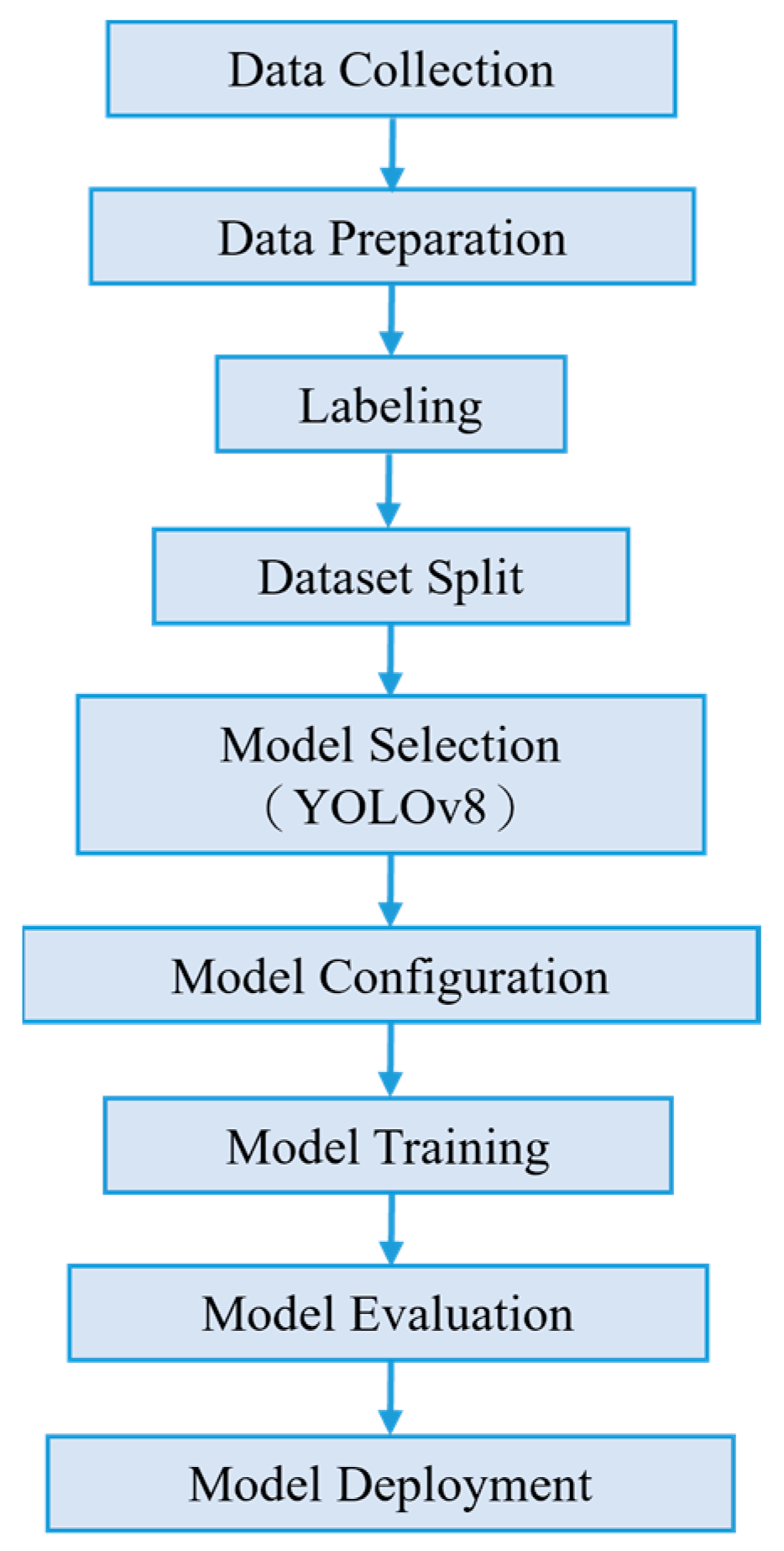
Furthermore, in this study, YOLO v8 was used to train a model for the purpose of identifying water-wheel tails. Since “water-wheel tails” are specific and not commonly found features, general pre-trained models are often trained on more common objects like humans, cats, dogs, cars, etc., and may not handle these data effectively. Therefore, in this research, training and prediction were carried out using a custom dataset to achieve the goal of recognizing water-wheel tails. The training process with the custom dataset is illustrated in
Figure 8.
To evaluate the detection performance of a water-wheel tail, we trained a machine learning model using YOLO v8. In classification or detection tasks, the confusion matrix is commonly used as an evaluation metric. It is a two-dimensional matrix where rows represent the actual labels and columns represent the model’s predicted results (as shown in
Table 2). Based on the confusion matrix, various commonly used evaluation metrics can be calculated, including precision, recall, and F1 score. Precision measures the accuracy of the model in predicting positives, with a higher proportion of true positives among all samples predicted as positive (refer to Equation (2)). Recall measures the predictive ability of the model for positive samples by correctly predicting more among all actual positives (refer to Equation (3)). The F1 score is a harmonic mean of precision and recall and is often used in imbalanced class problems. It also serves as one of the indicators for evaluating the accuracy of this water-wheel tail detection model. It provides a single metric to comprehensively assess model performance.
In the model training, the definition of the water-wheel tail, as shown in
Figure 9, differs slightly from the previous definition. To make it easier for the model to learn the complete characteristics of water-wheel tails, the starting point of the water-wheel tail was changed to the outer side of the water-wheel base, while the ending point remained the same as that of the previous definition for measuring the length of the water-wheel tail. To augment the dataset and improve its generalization, various data augmentation techniques were employed in this study, including random brightness adjustment, random saturation adjustment, horizontal flipping, 5-degree clockwise and counterclockwise rotations, random translation, random cropping, 90-degree clockwise and counterclockwise rotations, and the addition of Gaussian noise. The images before and after data augmentation are shown in
Figure 10. The original dataset consisted of 100 images of water-wheel tails without the calibration board (as shown in
Figure 11) and 10 images of water-wheel tails with the calibration board. After applying the 10 data augmentation techniques, the total dataset size increased to 1210 images. In this study, the dataset was split into 10% for testing and 90% for training and validation. The number of training epochs was set to 100, the batch size was set to 8, and the width and height of the image were adjusted to 640 pixels. A GPU was utilized for training.
3. Results
To verify the feasibility of the water-wheel tail measurement system, this study conducted experiments on both the effectiveness of projective transformation and the measurement of the water-wheel tail length.
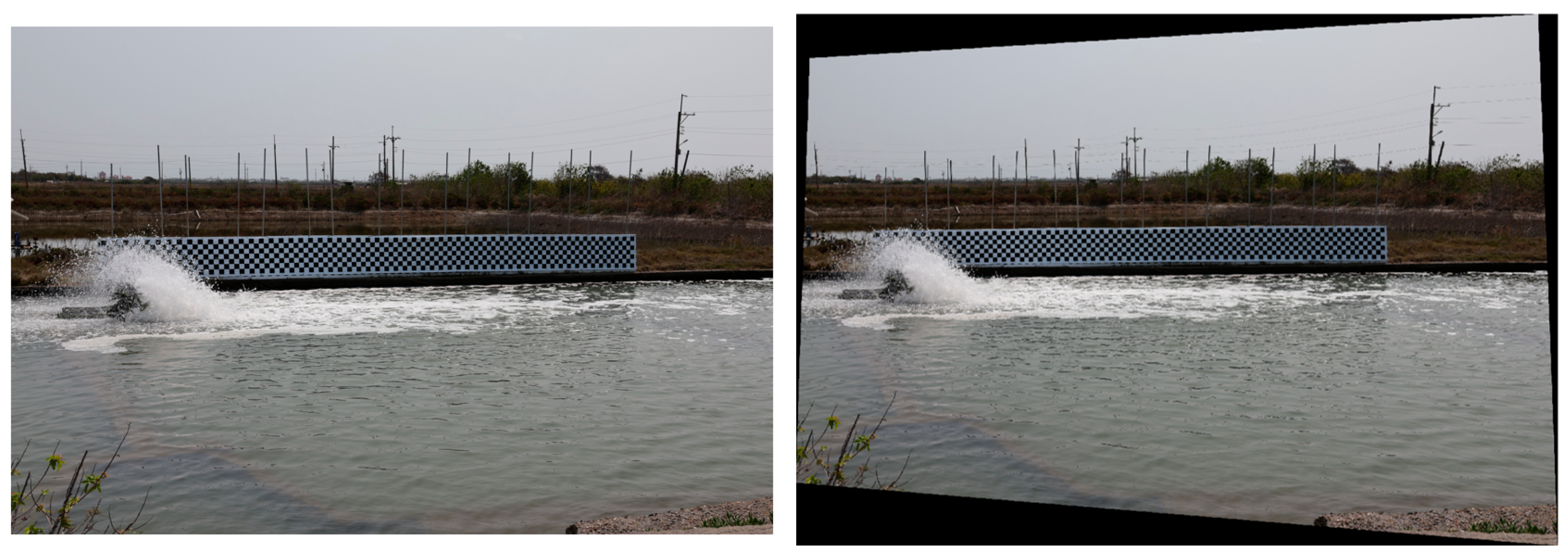
Figure 12 presents a side-by-side comparison of images before and after projective transformation, showcasing the successful correction of perspective distortion.
Table 3 and
Figure 13 display the results of the projective transformation validation using calibration boards of different specifications. These experiments, labeled “−1” and “−2”, represent the first and second experiments, respectively. The data obtained from different shooting positions were depicted in a graph, with the “No. of the picture” signifying the different images captured at the same position. Specification A had a theoretical value of 11.3 m, while specification B had a theoretical value of 11.232 m. The second experiment illustrated in
Figure 13, which involved changing the camera used for shooting from FUJIFILM FinePix HS10 to Canon EOS R10, demonstrated that the data in the second experiment were more concentrated compared to the first experiment. The standard deviation of the data also decreased. Moreover, the average percentage error for specification A was lower than that for specification B in both experiments, indicating that the calibration board of specification A had a better projective transformation effect in this experimental environment. However, it was noted that the measurement accuracy of the calibration boards met the expected goal of being smaller than 0.5 m in both experiments.
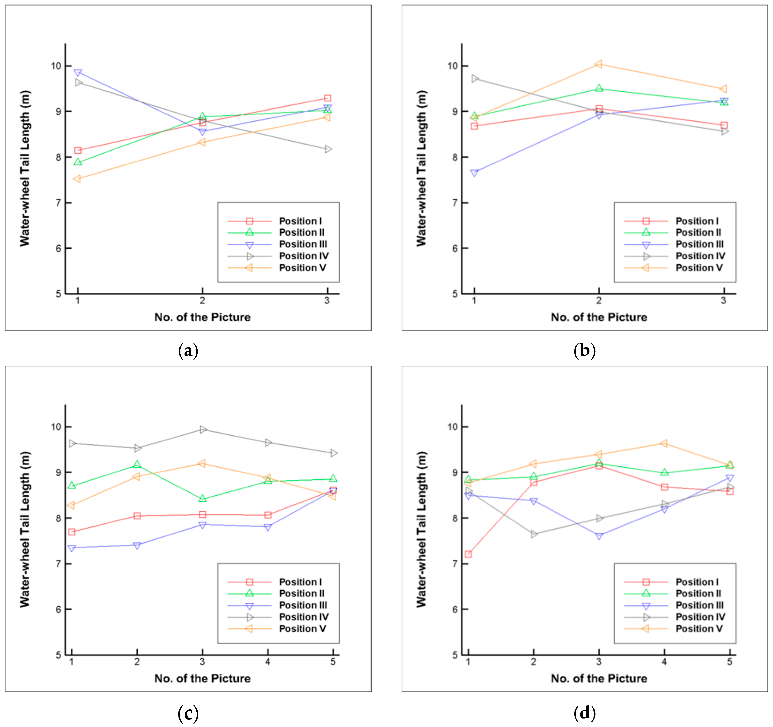
Figure 14 presents the outcomes of the water-wheel tail length measurement. It can be observed that most of the measured values fall within the 7 to 10 m range. For specification A in the first experiment, the maximum, minimum, and average values are 9.87 m, 7.52 m, and 8.72 m, respectively. In the first experiment with specification B, the maximum, minimum, and average values are 10.04 m, 7.67 m, and 9.04 m, respectively. In the second experiment, the values for specification A are 9.94 m, 7.35 m, and 8.62 m, while for specification B, they are 9.64 m, 7.21 m, and 8.66 m. The data concentration and the reasons behind it are further discussed in the next section.
Further, a model was trained to enable the recognition of the water-wheel tail feature.
Figure 15 depicts the training outcomes of the model, including the F1-epoch curve and the F1-Confidence curve. It is evident from
Figure 15a that the initial F1-score was around 0.6. After less than 10 training epochs, the F1-score surpassed 0.8, and it continued to rise gradually, converging to around 0.97. The highest F1-score achieved was 0.98098, occurring at the 86th training epoch. The average F1-score from the 51st to the 100th training epochs was 0.96713.
Figure 15b shows “all classes 0.97 at 0.589”, signifying that for all classes, when the model’s confidence was 0.589, the F1-score of the model reached 0.97. This implies that at a specific confidence threshold, the model performed very well in terms of positive predictions and correct detections.
Finally, when passing untrained images through the model for prediction, it can be observed that although the scenes are not identical, the model’s predicted bounding boxes still have a confidence level exceeding 0.8, and their boundaries closely align with the water-wheel tail as defined in this study, as shown in
Figure 16.
4. Discussion
The study reveals several important results related to the water-wheel tail measurement system. In the experiments involving projective transformation and calibration boards, the proposed system effectively corrected perspective distortion, with calibration board specification A demonstrating superior performance. The measurement accuracy of the calibration boards met the set expectations, confirming the system’s reliability.
The measurement of the water-wheel tail length showed that most values fell within the range of 7 to 10 m. However, some variations were observed, particularly as the water-wheel tail neared its endpoint. These variations were attributed to the dynamic nature of the water-wheel tail, where splashes and foam at the starting point led to challenges in maintaining a consistent length within a short time. Additionally, the calmer water flow at the tail’s endpoint made it susceptible to dispersion in different directions due to varying water currents and wind forces. As a result, fluctuations in the water-wheel tail’s length occurred over short periods, not solely due to water quality variations.
To improve the understanding of the correlation between the water-wheel tail length and water quality parameters, future efforts should involve multiple measurements at the same location. Applying averaging and other statistical methods can provide a more representative water-wheel tail length that accurately reflects the water quality at a given moment, while also minimizing potential biases stemming from a limited number of measurements.
The experimental results demonstrate the precise measurement capability of our system for the water-wheel tail in various scenarios. These initial findings have established a robust scientific foundation for our research. Our future work is to develop a real-time application tool that adheres to commercial standards, enabling continuous monitoring of water-wheel tails. This tool will encompass functionalities such as real-time data collection, analysis, and visualization, empowering users to monitor dynamic changes in the water-wheel tail promptly. We intend to dedicate the upcoming period toward developing and testing the system extensively to ensure its stability and usability.
5. Conclusions
This study developed a water-wheel tail length measurement system that uses projection transformation to correct input images and calculate coordinates in the transformed images. Through known conditions (such as the length of the water-wheel base) and proportional relationships, the actual length of the target object (such as the water-wheel tail) can be estimated. Two different-sized calibration boards were used for measuring the length of the chessboard edge and the water-wheel tail length, respectively, with the following results obtained. In the chessboard-edge length-measurement verification, it was found that the projection transformation effect using specification A was better, with an average error percentage of less than 0.25%. It was also confirmed that this system can be used with different camera modules, not being limited to specific cameras. In the water-wheel tail measurement experiment, it was found that the system could eliminate perspective distortion through projection transformation, and the transformed images could be used to measure water-wheel tail lengths in fish ponds, while the system could also capture the dynamic changes in water-wheel tail lengths.
By increasing the quantity and diversity of the dataset through data augmentation methods and training it with the YOLO v8 deep learning model, the model was able to recognize features of the water-wheel tail. In the final testing, the maximum mAP50 reached 0.99013, while the maximum mAP50-95 was 0.885. When predicting data that were already used for training purpose, except for the data augmentation method of a rotation by 90°, the confidence levels of other augmentation types exceeded 0.9. For the deployment results with untrained data, the confidence levels were also greater than 0.8, and the predicted bounding boxes were close to the water-wheel tail as defined in this study.


