Identification of the Representative Point for Soil Moisture Storage Using a Precipitation History Model

Abstract

Soil water storage is an essential variable in hydrological processes at the hillslope scale. This study proposed models for predicting soil water based on the precipitation history. According to the mathematical analysis of soil water storage on the hillslope scale, hydrological fluxes can be effectively expressed in terms of the weighted time series of precipitation and evapotranspiration. Moreover, the impact of evapotranspiration on soil water storage was incorporated into the model structure as an autoregressive process. A new soil water prediction model was developed through the integration of the soil moisture stochastic process into the structure of a precipitation-based model for the hillslope scale. Intensive soil moisture and rainfall data collected over two years were then used to test the performance of the developed models for two different hillslopes. The proposed model exhibited a better ability to find representative points for soil water storage than either existing precipitation-based models or the temporal stability method.

1. Introduction

Hydrological processes in mountainous hillslopes are very complicated due to the spatially variable slope, aspect, soil thickness, and texture as well as the temporally variable rainfall, vegetation, and presence or absence of snow. In order to characterize the variability in water storage at a hillslope scale, the soil moisture measurement can be used to explain various hydrological components in the context of the mass balance principle. Soil moisture plays a critical role in eco-hydrological processes that determine the relationship between precipitation and runoff [1]. Soil moisture monitoring is critical for understanding the hydrologic cycle, investigating hydrological processes, monitoring droughts, and developing landslide early warning systems [2]. Numerous attempts have been made to determine the temporal and spatial variations in soil moisture through both in situ sampling and remote sensing methods, whose respective strengths and weaknesses depend on the goal of the analysis [3]. Although in situ monitoring provides highly accurate soil moisture data, it often demands substantial sampling costs for spatial upscaling. Remote sensing using drones and satellites can cover large sampling areas but struggles to overcome detectability issues in deep soil layers and sensitivity to environmental factors such as climate, land use, and terrain conditions [4]. In order to upscale soil moisture obtained from in situ measurements, previous studies have focused on the selection of the available optimal points to characterize the spatiotemporal soil moisture distribution and represent the mean soil moisture variation in the hillslope area [5,6]. The representative point in a soil moisture network system is typically determined by the temporal stability method, which can be defined as the persistence of the spatial pattern of soil moisture in an area over time [7]. The correlation between environmental factors and soil moisture measurements has been explored using clustering and orthogonal-function-based approaches [8].

The temporal stability method has been widely used to characterize the temporal–spatial distribution of measurements in a soil moisture network and obtain the representative point from hillslope to watershed scale [6,7]. The spatial distribution of temporal stability can be influenced by various parameters (e.g., soil properties, depths, land cover, soil condition, and network scale) [9]. Clustering analysis to find optimal clusters with similar characteristics has been conducted for the selection of the representative point by considering the relationship with terrain indices and soil properties [5]. The statistics of a soil moisture network, such as the number of sampling points and the observation period, plays a primary role in the selection of the representative point and also substantially affects the determination of the number of representative points. Previous studies mostly focused on identifying the representative point based on multiple time series datasets in the soil moisture network. However, the soil water storage (SWS) can be important to represent the potential of runoff as well as the wetness status of the watershed or hillslope [8,9].

The antecedent precipitation index (API) was introduced to consider the impact of precipitation history in water balance on SWS [10]. The API model has been used to estimate the runoff coefficient and measure the antecedent soil moisture in rainfall–runoff modeling [11]. However, the API considers neither evapotranspiration nor critical hillslope hydrological processes. In other word, the potential of soil moisture measurement is not necessarily limited to the optimization of API parameters. The representation of eco-hydrological processes can be implemented into the time series model for soil water prediction.

The recession characteristics of soil moisture in root zones have been explained by soil water loss due to evapotranspiration [12]. Estimation of the memory structure was conducted by calculating the time-lagged autocorrelation function and was represented as a first-order Markov process and autoregressive term [13]. In reality, time series analysis of soil moisture has been applied to determine the water balance under the soil layer from the hillslope scale to the global scale [14]. The memory structure of soil moisture has been used to improve the performance of climate models in the context of seasonal forecasts and to understand the connectivity between soil moisture at the hillslope scale [15].

Considering that the soil water memory can originate from evapotranspiration and other hydrological processes under the soil layer, integration of the soil moisture memory into the model structure seems a reasonable approach in terms of precipitation models. This can be useful for addressing the responsive mechanism for the soil water process as well as for improving the prediction of soil moisture. Therefore, this study proposes an innovative prediction method for soil water considering the eco-hydrological relationships and hydrological processes under the soil layer in terms of a stochastic model at the hillslope scale. An alternative method for the selection of the soil water representative point was also developed by introducing the similarity in the soil moisture stochastic process. In order to validate the developed method, time series of soil moisture, precipitation, and evapotranspiration were collected for two years in two different humid mountainous hillslopes. Three model development research objectives and their applications were addressed in this study.

First, a stochastic process to consider the memory characteristics in the mass balance of SWS under soil layer was derived and implemented as the basis of a precipitation history model to address the response characteristics of soil moisture time series data.

Second, an innovative method to determine the representative point was proposed in the soil moisture monitoring network, considering the similarity in stochastic processes with the average of SWS at the hillslope scale in comparison with the representative point approach based on the temporal stability method.

Thirdly, the soil water prediction performances of the developed models were compared with some existing precipitation-based models. These three objectives demonstrate the potential of the proposed method in the selection of the representative point based on the stochastic hydrological processes as well as better prediction of SWS at the hillslope scale.

2. Materials and Methods

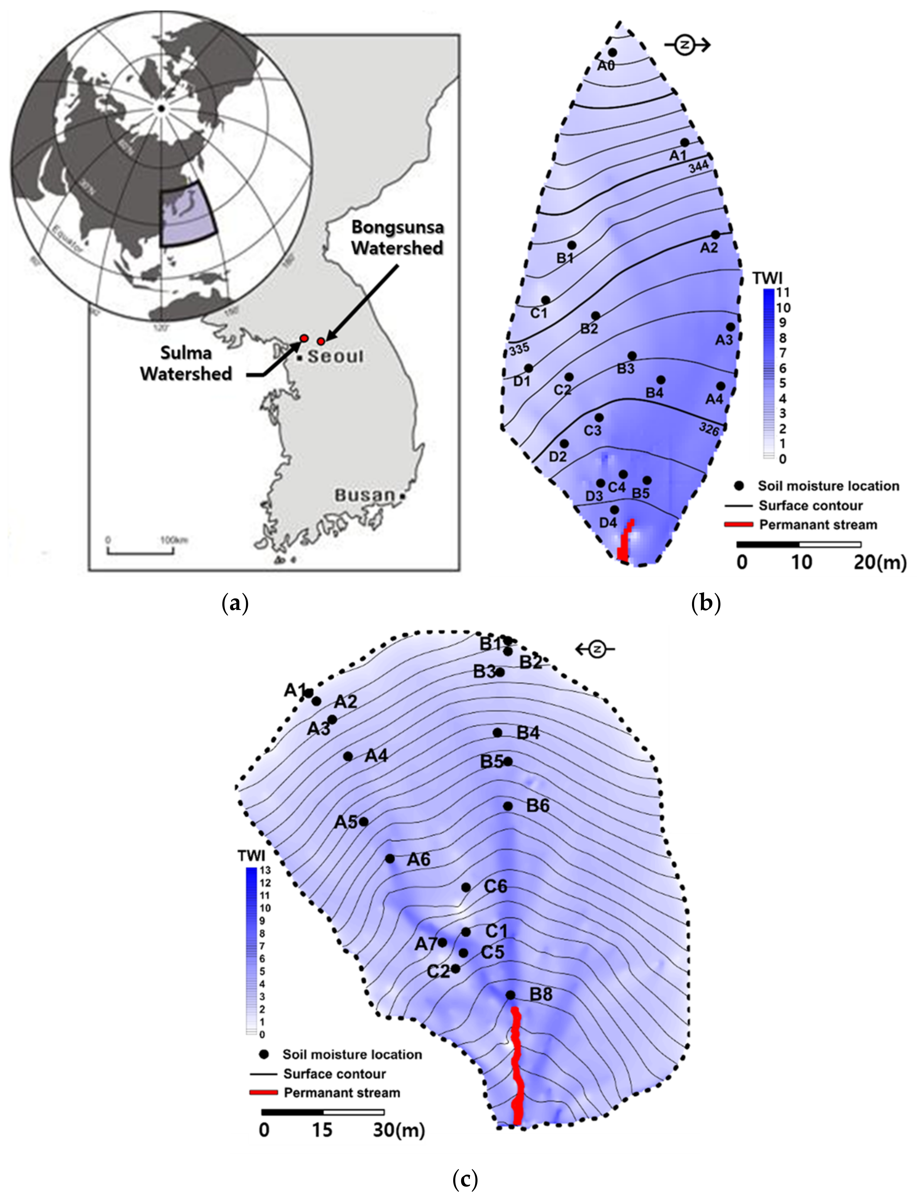
2.1. Study Area

One of the study areas was a steep hillslope (hillslope B) inside the Bongsunsa catchment (37°45′25.37″ N and 127°9′11.62″ E) in Pochun-si, and the other was a headwater hillslope (hillslope S) in the Sulmachun catchment (37°56′19.99″ N and 126°57′16.94″ E) in Paju-si, Gyeonggi-do, Republic of Korea (Figure 1).

Hillslope B was underlain by weathered gneiss and schist with an eastern aspect (dipping to the east), whereas gneiss composites underlain by granite bedrock were the primary characteristic for hillslope S (dipping to the west). The average annual temperatures over the last five years were 11.5 °C and 10 °C, and the mean annual rainfall was approximately 1400 mm and 1067 mm at hillslopes B and S, respectively. More than 65% of the annual rainfall occurs between June and August due to the Asian monsoon. The areas of hillslope B and S were approximately 2100 m² and 4000 m², and the average slopes were 19° and 28°, respectively. The soil texture was commonly a mixture of sandy loam and loamy sand with sand (43–65%), silt (29–46%), and clay (6–11%) on hillslope B and sandy loam and loamy sand with sand (57–76%), silt (22–38%), and clay (5–10%) on hillslope S, respectively, based on soil taxonomy (USDA). Both hillslopes exhibited abundant macropores in the topsoil on visual inspection. The mean soil porosities were 49.6% and 48% for hillslopes B and S, respectively. The soil thickness of hillslope B was 40–100 cm and that of hillslope S was 25–90 cm [15,16]. The soil layer on hillslope B was well distributed between the upslope and downslope, whereas the spatial distribution of soil thickness was relatively uneven on hillslope S. A canopy mixture of Carpinus sp. and shrubby Quercus sp. was the primary land cover on hillslope B, with no notable spatial distribution of vegetation communities. Hillslope S was covered by a mixture of Polemoniales, shrubby Quercus sp., and a coniferous canopy of Pinus densiflora. A flux tower is located 300 m downstream of hillslope B, which has been operating since 2005, collecting fluxes of H₂O and CO₂ through the eddy covariance technique [17]. Evapotranspiration data were also obtained using the eddy covariance method at a flux tower 50 m from hillslope S.

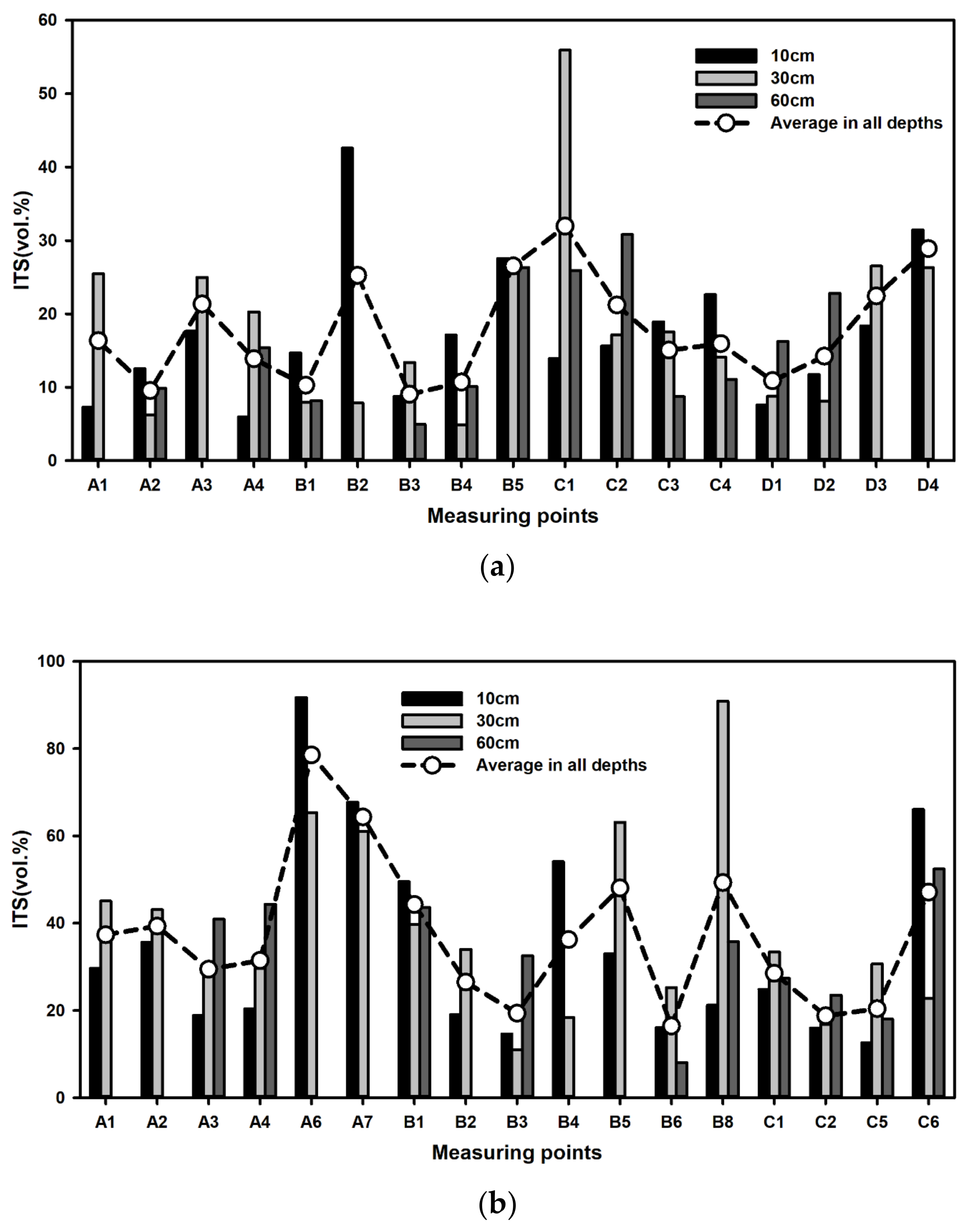
2.2. Acquiring Hydrologic Data on the Hillslope

The spatial distributions of wetness tendency (e.g., the upslope contributing area and topographic wetness index (TWI)) and the soil depth distribution were considered when selecting monitoring locations for the soil moisture sensor network. As presented in Figure 1b,c, the TWI was calculated and used to delineate the location of soil moisture sensors considering the saturation tendency along the hillslope [15,16]. The topography is a dominant control factor on the redistribution of soil water throughout hillslope B. As shown in Figure 1, soil moisture measurement points were allocated along transects based on digital terrain analysis. A long-term soil moisture monitoring system was installed on the hillslope, considering the operational scale of the wired time domain reflectometry (TDR) system (<100 m) [18]. For hillslope B, time series soil moisture data were collected at 18 monitoring locations along four transects (A, B, C, and D), with 12 locations at three depths (10, 30, and 60 cm), 5 locations at two depths (10 and 30 cm), and 1 location (A0) with extremely low data quality, depending on the soil layer depths (Figure 1b). Time series soil moisture data were collected at 44 points on hillslope S. Depending on the soil depth, two or three waveguides were inserted into the upslope direction along two transects (A and B) and region C, as shown in Figure 1c. The soil moisture data were collected every 2 h, with a 40 min TDR operation time and an hour or longer for the machine to cool down. Occasionally, the soil moisture data suffered from unpredictable interruptions (e.g., the TDR cable being damaged by rodents or the machine being damaged by lightning). Considering the operational temperature of the TDR (>0 °C), no soil moisture monitoring was performed between December and March. The soil moisture data collected between 2009 and 2011 for hillslope B and between 2015 and 2016 for hillslope S were used for the analysis, which indicated a very high rate (≈100%) of successful data acquisition. Rainfall, evapotranspiration, and temperature were measured at the flux tower [19].

2.3. Mathematical Development for Soil Water Storage

The temporal variation in SWS is important for evaluating the impact of rainfall on the spatial distribution of water storage in a soil layer. The SWS can be approximated by multiplying the soil moisture by the corresponding soil depth. If the soil moisture is measured at three depths (e.g., 10, 30, and 60 cm), the SWS values for the depth profiles can be expressed as $R_{t, 0-20}\left(\mathrm{mm}\right)={\theta }_{t,10\mathrm{cm}}\ast 200 \mathrm{mm}, R_{t, 0-45}\left(\mathrm{mm}\right)=R_{t, 0-20}+{\theta }_{t,30\mathrm{cm}}\ast 250 \mathrm{mm}$, and $R_{t, 0-80}\left(\mathrm{mm}\right)=R_{t, 0-45}+{\theta }_{t,60\mathrm{cm}}\ast 350 \mathrm{mm}$, which represent the water storage for the surface zone, root zone, and total soil layer, respectively.

The mass balance relationship for two sequential SWS areas ($R_t$ and $R_{t-1}$ for time steps t and t − 1), as well as other hydrological components such as evapotranspiration ($E{T}_t$) and precipitation ($P_t$) for a regolith at a hillslope location, can be expressed as a function of the lateral flow from the upslope ($u_t$), the lateral flow to the downslope ($l_t$) area, and the percolation to a deeper layer ($v_t$):

$$R_t=P_t-E{T}_t+f_t·R_{t-1}$$

(1)

where $f_t=u_t-l_t-v_t$ is the fraction of water storage from the previous time step. A similar development of a soil moisture time series has been performed in [14].

By introducing $f_t=f$ to simplify the derivation, the sequential developments in Equation (1) provide the SWS at t as a function of the precipitation and evapotranspiration history as follows:

$$R_t={{\displaystyle \sum }}_{i=1}^t{f}^{t-i}{P}_i-{{\displaystyle \sum }}_{i=1}^t{f}^{t-i}E{T}_i+f^t{R}_0$$

(2)

Considering the initial water storage impact and soil layer thickness for different depth profiles, Equation (2) can then be approximated as follows:

$$R_t\cong {{\displaystyle \sum }}_{i=1}^t{f}^{t-i}{P}_i-{{\displaystyle \sum }}_{i=1}^t{f}^{t-i}E{T}_i+C_0$$

(3)

where $C_0$ is the impact of the initial SWS for the designated regolith.

2.4. Prediction of Soil Moisture Using Rainfall History

The soil moisture has previously been predicted by merging the weighted history of precipitation, i.e., the API, into several regression models as follows [20]:

$$S_t=a+b·{{\displaystyle \sum }}_{i=1}^N{w}_i{P}_{t-i}$$

(4)

$$S_t=a+b·\left(1-e^{-c·\left({{\displaystyle \sum }}_{i=1}^N{w}_i{P}_{t-i}\right)}\right)$$

(5)

$$S_t=a·\frac{{({{\displaystyle \sum }}_{i=1}^N{w}_i{P}_{t-i})}^{1.5}+b}{{\left({{\displaystyle \sum }}_{i=1}^N{w}_i{P}_{t-i}+b\right)}^{1.5}}+c$$

(6)

where $S_t$ is the soil moisture time series; a, b, and c are fitted coefficients; $N$ is the number of days; $P_{t-i}$ is precipitation at the time step t – i; and $w_i$ indicates the weighting factors for soil moisture recession.

By applying the exponential function to the soil moisture time series data, the impact of the weighted precipitation history can be expressed as follows:

$${{\displaystyle \sum }}_{i=1}^N{w}_i{P}_{t-i}=K{{\displaystyle \sum }}_{i=1}^N{w}_i{P}_{t-i-1}+P_t$$

(7)

where the damping factor K ranges from 0.80 to 0.98 [19].

The sequential application of Equation (7) provides an expression for weighted precipitation accumulation into multiples of K to precipitation summation, i.e., the precipitation history impact (PHI), with an assumption of negligible impact of initial precipitation ($P_0\approx 0$), as follows:

$${{\displaystyle \sum }}_{i=1}^N{w}_i{P}_{t-i}={{\displaystyle \sum }}_{i=1}^t{K}^{t-i}{P}_i$$

(8)

2.5. Stochastic Model for the Difference between PHI and SWS

Equations (3) and (8) indicate that the difference in mathematical expressions between the weighted precipitation history and SWS can be expressed as the weighted history of evapotranspiration. Several studies have previously explained the time series features of soil moisture using those of evapotranspiration [12,13].

In order to effectively address the difference ($e_t$) between Equations (3) and (6), an autoregressive model can be introduced as follows:

$$R_t={{\displaystyle \sum }}_{i=1}^t{K}^{t-i}{P}_i+e_t, e_t\approx AR\left(p\right)=-{\varnothing }_1{e}_{t-1}-{\varnothing }_2{e}_{t-2}-\cdots -{\varnothing }_7{e}_{t-p}$$

(9)

where p is the order of the highest lag for the autoregressive model.

In this study, we used seven days (a week) for p through heuristic modeling. The statistical test for significance was applied to all coefficients in the autoregressive model (Equation (9)). The modeling result was checked using a chi-squared test for the residual of Equation (9) to secure the white noise feature in the residuals.

If a similar procedure to Equation (8) is applied to the time series data of evapotranspiration, the summation of the weighted evapotranspiration time series can be expressed as follows:

$${{\displaystyle \sum }}_{i=1}^N{w}_i^{\prime }E{T}_{t-i}={{\displaystyle \sum }}_{i=1}^t{\left(K^{\prime }\right)}^{t-i}E{T}_i$$

(10)

where $w_i^{\prime }$ and $K^{\prime }$ are the weighting factor and damping factor for evapotranspiration, respectively.

The analogy between the autoregressive model (Equation (9)) and actual evapotranspiration can be further explored using measurements of evapotranspiration from the flux tower. By introducing the assumption that K in Equation (9) is identical to $K^{\prime }$ in Equation (10) based on Equation (3), the distinct time series of evapotranspiration components between the hillslope soil layer and flux tower can be modeled. In other words, the stochastic structures from Equation (9) and those from Equation (10) can be compared to identify the possible causality between the difference ($e_t$) and the evapotranspiration.

3. Results

3.1. Relationship between SWS and PHI

The $R_t$ in Equation (9) can be predicted in terms of ${{\displaystyle \sum }}_{i=1}^t{K}^{t-i}{P}_i$ in Equation (8) to evaluate the impact of precipitation memory on the spatial average SWS at depths of 20, 45, and 85 cm. The parameters (K) in the PHI model were calibrated using an objective function to maximize the coefficient of determination between the observation and prediction values of SWS.

Table 1. Calibrated K coefficients and predictabilities in the PHI model for soil water storage (SWS) at all depths (20 cm, 45 cm, and 80 cm) for the two hillslopes.

Hillslope		B			S
soil depth for storage		20 cm	45 cm	80 cm	20 cm	45 cm	80 cm
coefficient K		0.83	0.85	0.87	0.93	0.94	0.95
calibration data	${\mathrm{R}}^2$	0.66	0.56	0.54	0.42	0.42	0.44
	$\mathrm{RMSE}$	41.07	45.37	51.2	35.67	35.85	73.99
validation data	${\mathrm{R}}^2$	0.57	0.54	0.57	0.34	0.34	0.35
	$\mathrm{RMSE}$	90.36	99.85	113.08	23.80	40.18	92.19

Note: R²: coefficient of determination; RMSE: root mean square error.

presents the calibrated Ks for SWS at soil depths of 20, 45, and 85 cm, which were 0.83, 0.85, and 0.87 for hillslope B and 0.93, 0.94, and 0.95 for hillslope S. The higher Ks for hillslope S indicates a slower flux for hillslope S. These values correspond to known parameter ranges (between 0.8 and 0.98) reported in other studies [19]. The contribution to evaporation is different between surficial and deeper layers. Greater depths correspond to higher K values in both sampling sites, which indicates that the memory impacts of precipitation on SWS are more significant at greater depths, which are continuously affected by not only precipitation inputs but also soil water flow from upper depths and upslope areas. The predictability of the PHI model in terms of R² and root mean square error (RMSE) in the validation dataset is lower than that in the calibration dataset for both hillslopes (see Table 1), indicating high sensitivity and uncertainty in K for the difference in rainfall features between the two datasets.

3.2. Stochastic Models for the Difference between PH and SWS

The difference between the PHI model and SWS values at various soil depths can be properly addressed through the implementation of an evapotranspiration component, as illustrated in Equations (3) and (8). An autoregressive model was introduced to address the difference ($e_t$) in Equation (9). The standard procedure for time series modeling (e.g., checking the data, investigating the memory structure, building the model structure, parameter estimation, and diagnostic checking) [21] was applied using a maximum lag order of seven days.

Table 2. Estimated parameters and SP models for SWS at depths of 20 cm, 45 cm, and 80 cm for all monitoring points and residual tests for hillslope B. Black dots (●) represent the residual as white noise through a χ² test; the rings (○) denote stochastic structures in the residuals.

20 cm	Avg	A1	A2	A3	A4	C1	C2	C3	C4
AR(1)	0.82	0.88	0.94	0.66	0.48	1.08	0.94	0.57	0.69
AR(2)						−0.14
AR(3)	0.16			0.15	0.26			0.42
AR(4)	−0.24							−0.34	−0.27
AR(5)	0.18							0.23	0.29
${\mathit{\chi }}^2$	●	●	●	○	○	●	●	●	○
45 cm	Avg	A1	A2	A3	A4	C1	C2	C3	C4
AR(1)	0.83	0.9	0.95	0.71	0.47	0.96	1.10	0.65	0.70
AR(2)							−0.15
AR(3)	0.14			0.13	0.23			0.36
AR(4)	−0.18							−0.35	−0.30
AR(5)	0.15				0.11			0.25	0.27
${\mathit{\chi }}^2$	●	●	●	○	○	●	●	●	○
80 cm	Avg	A1	A2	A3	A4	C1	C2	C3	C4
AR(1)	0.82		0.95		0.57	0.97	1.12	0.70	0.72
AR(2)							−0.17
AR(3)	0.18				0.20			0.35
AR(4)	−0.19							−0.39	−0.27
AR(5)	0.15				0.12			0.28	0.25
${\mathit{\chi }}^2$	●		●		○	●	●	●	○
20 cm	B1	B2	B3	B4	B5	D1	D2	D3	D4
AR(1)	0.93	0.93	0.88	0.67	0.74	0.91	0.94	0.76	0.62
AR(2)							−0.22
AR(3)				0.18			0.12		0.21
AR(4)					−0.26			−0.19	−0.29
AR(5)					0.25			0.31	0.25
${\mathit{\chi }}^2$	●	●	●	●	○	●	●	○	●
45 cm	B1	B2	B3	B4	B5	D1	D2	D3	D4
AR(1)	0.96	0.96	0.85	0.65	0.76	0.94	0.97	0.82	0.67
AR(2)							−0.21
AR(3)				0.21			0.14		0.24
AR(4)					−0.29			−0.21	−0.23
AR(5)					0.24			0.32	0.25
${\mathit{\chi }}^2$	●	●	●	●	○	●	●	○	○
80 cm	B1	B2	B3	B4	B5	D1	D2	D3	D4
AR(1)	1.01		0.90	0.62	0.79	0.95	0.93
AR(2)
AR(3)				0.15
AR(4)	−0.18				−0.25
AR(5)	0.13			0.13	0.21
${\mathit{\chi }}^2$	●		●	●	○	●	●

presents the autoregressive parameters (${\varnothing }_1,\dots {\varnothing }_5)$ of stochastic precipitation (SP) models for all locations at three soil depths (20, 45, and 80 cm). All evaluated parameters presented in Table 2 were statistically significant (p < 0.05). As presented in Table 2, all autoregressive parameters were distributed at lags of one to five days. While parameters for odd orders had positive and high estimates, those for even orders are negative and exhibited smaller magnitudes than their prior order parameter, except for point B3 at a depth of 80 cm at hillslope S (Table 2). There was a distinct feature of autoregressive parameter dependence on spatial characteristics such as slope location and depth at hillslope B. While the structure of autoregressive models was simpler in upslope areas and at shallower depths, such as at locations A1, B1, C1, and D1 at depths of 20 and 45 cm, those for downslope areas (e.g., locations A4, B5, C4, and D4) exhibited multiple-term models with high orders at hillslope B. However, the model structures for many measurement points at hillslope S were identified as the AR(1) model and did not show a significant relationship with measurement depth and location (not presented). Although the majority of model residuals passed the assumption of residual independence for time series modeling, as presented in Table 2, the residuals of autoregressive models for deeper and downslope locations occasionally failed the ${\mathit{\chi }}^2$ test checking for white noise at hillslope B, indicating that the corresponding hydrological processes can be highly complicated, which can be associated with the heterogeneity in subsurface lateral flow. The development of macropores and lesser cracking of the bedrock can result in an uneven generation of lateral flow in the downslope part.

The impact of evapotranspiration on SWS is presented in Equation (3) with the accumulated impact of rainfall, which is similar to the representation of the PHI model, for example, in Equation (8). The impact of evapotranspiration can be considered in the model with the ET formulation, which is shown in Equation (10). As presented in Equations (3) and (10), the SWS can be independently affected by precipitation and evapotranspiration. The time series of the difference, $e_t$, in Equation (9) and the weighted evapotranspiration from the flux tower using calibrated Ks (Table 1) in Equation (10) can be obtained at three different depths for the two hillslopes, respectively.

The time series of Equation (10) was modeled for a comparison with the stochastic structure of the difference between SWS and precipitation. The statistics of the two different time series indicate that the mean values were similar between Equations (9) and (10) for the two different hillslopes (

Table 3. Statistical parameters of e_t in Equations (9) and (10).

Hillslope	Datasets		Mean	Median	Standard Deviation	Max.	Min.
B	20 cm SWS	$e_t$ Equation (9)	27.74	16.19	38.25	245.14	−0.01
		Equation (10)	28.82	33.05	18.20	58.25	0.55
	45 cm SWS	$e_t$ Equation (9)	31.82	24.45	35.16	229.01	−1.16
		Equation (10)	32.65	37.22	20.47	65.17	0.55
	80 cm SWS	$e_t$ Equation (9)	36.31	30.93	33.15	214.02	−1.87
		Equation (10)	37.66	43.82	23.41	74.08	0.55
S	20 cm SWS	$e_t$ Equation (9)	41.83	31.47	33.45	186.63	−2.35
		Equation (10)	44.97	52.08	21.27	78.32	0.69
	45 cm SWS	$e_t$ Equation (9)	51.61	44.72	30.90	174.85	−5.58
		Equation (10)	52.27	60.16	24.19	89.59	0.69
	80 cm SWS	$e_t$ Equation (9)	65.66	70.32	30.34	156.79	−10.59
		Equation (10)	62.43	71.02	28.75	104.86	0.69

). Although the medians were less than the means for $e_t$ in Equation (9), the medians were greater than the means of Equation (10) in all datasets; the standard deviations of $e_t$ in Equation (9) were also greater than those in Equation (10), as shown in Table 3. This means that the statistical distribution of $e_t$ in Equation (9) is more dispersed than that of $e_t$ in Equation (10), which is confirmed by the minimum and maximum values in Table 3. This can be explained by the fact that the residuals between the rainfall series and the weighted soil moisture address additional hydrological processes over evapotranspiration.

3.3. Representative Points Based on the Stochastic Process of SWS and Temporal Stability

Temporal stability has been widely used to determine the representative points for estimating the soil moisture average based on the time-invariant relationship between spatial locations. A temporal stability analysis was conducted on the spatiotemporal relationship between the soil moisture time series to estimate the average soil moisture, whereas the SP model considers the time series characteristics between rainfall characteristics and soil moisture. In order to find the representative point for soil moisture, the index of temporal stability (ITS) was computed at three different depths in the two study areas. The representative point for all depths was also determined using the mean soil moistures for specific locations. As shown in Figure 2, the lowest ITS values for all depths were identified as point B3 and point B6 for hillslopes B and S, respectively.

The difference between SWS and multiples of K in the precipitation time series in Equation (9) can be modeled using autoregressive models. Table 2 presents the distribution of models for all points at three depths for both hillslopes. The spatially different delineated autoregressive models address the local soil moisture response features, such as connectivity to upslope areas and nonlinear soil water flow paths, which can be characterized through combinations of matrix and macropore flows. The time series data of spatially averaged soil moisture for three different depths can be used to model the differences. The model structure for hillslope B was formulated using AR(1), AR(3), AR(4), and AR(5), whereas that for hillslope S consisted of the AR(1) term. The difference in soil layer development and soil water flow path between the two hillslopes may explain the different model structures.

A soil moisture monitoring point can be identified according to the similarity of the model structure and its parameter estimates. The delineated model for point C3 exhibited an identical distribution in model terms and similar parameter estimates to those for spatially averaged soil moisture at all three depths for hillslope B. Similarities between the models for average soil moisture and those for point C6 were also identified at hillslope S. Both points satisfy the white noise assumption in model residuals. If the stochastic structures between different time series are identical, a reliable relationship from one to another can be established. In other words, the stochastic process at point C3 and point C6 for hillslope B and hillslope S, respectively, can represent the mean soil water memory impact for the average SWS of all measurement points at depths of 20, 45, and 80 cm.

The degree of representativeness can be evaluated through the correlation between average SWS and SWS for a selected point. Figure 3a,c show linear relationships between average SWSs and those of points C3 and C6 at hillslopes B and S, respectively. Similar relationships for points B3 and B6, identified through conventional stability analysis, are presented in Figure 3b,d for hillslopes B and S, respectively. The SP model resulted in higher R² values than the conventional temporal stability analysis for the linear relationships between average SWS and the selected point at selected points.

Table 4. Representative points determined by the similarity between the stochastic model of SWS and temporal stability and their regression relationship to average SWS with R² and RMSE.

Hillslope	Dataset	Point	Calibration		Validation
			${\mathit{R}}^2$	$\mathbf{RMSE}$	${\mathit{R}}^2$	$\mathbf{RMSE}$
B	20 cm SWS	C3	0.83	2.99	0.86	4.84
		B3	0.74	3.65	0.83	9.06
	45 cm SWS	C3	0.82	6.03	0.89	8.77
		B3	0.77	6.86	0.87	12.10
	80 cm SWS	C3	0.83	8.95	0.93	10.50
		B3	0.81	9.42	0.89	18.40
S	20 cm SWS	C6	0.95	1.64	0.90	2.59
		B6	0.94	1.74	0.90	4.05
	45 cm SWS	C6	0.96	3.54	0.96	5.06
		B6	0.93	4.43	0.92	6.33
	80 cm SWS	C6	0.96	6.28	0.98	8.00
		B6	0.94	7.28	0.92	8.95

presents the model performances (R² and RMSE) for calibration and validation between the spatially averaged SWS and the SWS for the representative point at three depths for the two hillslopes. The representative points based on the stochastic processes of SWS exhibited higher R² and lower RMSE than those based on temporal stability in both the training dataset (calibration) and the testing set (validation) (Table 4).

The higher accuracy of the representative point for SWS determined by the SP model can be attributed to the fact that the similarity in the stochastic process of the time series and the evapotranspiration process were both considered when identifying the best location for SWS evaluation. This means that the proposed SP model can be used as an identification method for representative locations of SWS at the hillslope scale.

4. Discussion

4.1. Predictability of SWS

The evaluation of SWS using precipitation characteristics can be useful simply because precipitation data are feasibly available and less cost demanding. While PHI and the existing models require precipitation history, the soil moisture at a representative point needs to be measured for the SP model (

Table 5. Predictabilities (R² and RMSE) of SWS using existing regression models (Lin.: linear; Exp.: exponential; [20] empirical) and the stochastic precipitation (SP) model. SP(C3) is the SP model from point C3.

Hillslope	Dataset		Model	PHI (K)	Lin.	Exp.	Empirical [20]	SP	SP (C3)
			Input Variables	$\mathit{A}\mathit{M}{\mathit{O}}_{\mathbf{1}\mathbf{,}\mathbf{\cdots }\mathbf{,}\mathit{t}}$	$\mathit{A}\mathit{M}{\mathit{O}}_{\mathbf{1}\mathbf{,}\mathbf{\cdots }\mathbf{,}\mathit{t}}$	$\mathit{A}\mathit{M}{\mathit{O}}_{\mathbf{1}\mathbf{,}\mathbf{\cdots }\mathbf{,}\mathit{t}}$	$\mathit{A}\mathit{M}{\mathit{O}}_{\mathbf{1}\mathbf{,}\mathbf{\cdots }\mathbf{,}\mathit{t}}$	$\mathit{A}\mathit{M}{\mathit{O}}_{\mathbf{1}\mathbf{,}\mathbf{\cdots }\mathbf{,}\mathit{t}}$${\overline{\mathit{\theta }}}_{\mathit{t}\mathbf{-}\mathit{k}}$	$\mathit{A}\mathit{M}{\mathit{O}}_{\mathbf{1}\mathbf{,}\mathbf{\cdots }\mathbf{,}\mathit{t}}$${\mathit{\theta }}_{\mathbf{1}\mathbf{,}\mathbf{\cdots }\mathbf{,}\mathit{t}}$
B	20 cm SWS	calibration 2009	${\mathrm{R}}^2$	0.66	0.66	0.68	0.67	0.93	0.83
			$\mathrm{RMSE}$	44.55	4.16	4.10	4.12	1.85	3.03
		validation 2011	${\mathrm{R}}^2$	0.57	0.57	0.71	0.73	0.93	0.78
			$\mathrm{RMSE}$	83.48	8.37	6.03	5.81	3.05	5.50
	45 cm SWS	calibration 2009	${\mathrm{R}}^2$	0.63	0.63	0.63	0.63	0.94	0.80
			$\mathrm{RMSE}$	89.44	8.68	8.60	8.58	3.35	6.36
		validation 2011	${\mathrm{R}}^2$	0.57	0.57	0.68	0.71	0.94	0.83
			$\mathrm{RMSE}$	101.46	16.20	12.48	11.89	5.42	9.75
	80 cm SWS	calibration 2009	${\mathrm{R}}^2$	0.61	0.61	0.62	0.62	0.95	0.80
			$\mathrm{RMSE}$	170.67	13.45	13.36	13.26	4.78	9.67
		validation 2011	${\mathrm{R}}^2$	0.57	0.57	0.67	0.71	0.94	0.88
			$\mathrm{RMSE}$	168.22	23.91	18.67	17.55	7.83	12.22
Hillslope	Dataset		Model	PH (K)	Lin.	Exp.	Empirical [20]	SP	SP (C6)
			Input Variables	$\mathit{A}\mathit{M}{\mathit{O}}_{\mathbf{1}\mathbf{,}\mathbf{\cdots }\mathbf{,}\mathit{t}}$	$\mathit{A}\mathit{M}{\mathit{O}}_{\mathbf{1}\mathbf{,}\mathbf{\cdots }\mathbf{,}\mathit{t}}$	$\mathit{A}\mathit{M}{\mathit{O}}_{\mathbf{1}\mathbf{,}\mathbf{\cdots }\mathbf{,}\mathit{t}}$	$\mathit{A}\mathit{M}{\mathit{O}}_{\mathbf{1}\mathbf{,}\mathbf{\cdots }\mathbf{,}\mathit{t}}$	$\mathit{A}\mathit{M}{\mathit{O}}_{\mathbf{1}\mathbf{,}\mathbf{\cdots }\mathbf{,}\mathit{t}}$${\overline{\mathit{\theta }}}_{\mathit{t}\mathbf{-}\mathit{k}}$	$\mathit{A}\mathit{M}{\mathit{O}}_{\mathbf{1}\mathbf{,}\mathbf{\cdots }\mathbf{,}\mathit{t}}$${\mathit{\theta }}_{\mathbf{1}\mathbf{,}\mathbf{\cdots }\mathbf{,}\mathit{t}}$
S	20 cm SWS	calibration 2015	${\mathrm{R}}^2$	0.41	0.41	0.47	0.50	0.95	0.90
			$\mathrm{RMSE}$	35.66	5.57	5.28	5.14	1.55	2.08
		validation 2016	${\mathrm{R}}^2$	0.33	0.33	0.37	0.40	0.87	0.81
			$\mathrm{RMSE}$	23.79	6.74	6.69	6.59	2.53	3.29
	45 cm SWS	calibration 2015	${\mathrm{R}}^2$	0.42	0.42	0.47	0.50	0.96	0.91
			$\mathrm{RMSE}$	35.85	12.73	12.13	11.81	2.72	4.46
		validation 2016	${\mathrm{R}}^2$	0.33	0.33	0.37	0.39	0.88	0.86
			$\mathrm{RMSE}$	40.17	16.02	15.90	15.65	5.52	7.17
	80 cm SWS	calibration 2015	${\mathrm{R}}^2$	0.43	0.43	0.46	0.48	0.96	0.92
			$\mathrm{RMSE}$	73.38	23.17	22.59	22.07	4.50	7.79
		validation 2016	${\mathrm{R}}^2$	0.34	0.34	0.36	0.38	0.87	0.87
			$\mathrm{RMSE}$	92.12	30.08	29.88	29.41	10.61	12.23

Note: R²: coefficient of determination; RMSE: root mean square error.

). The performances of the PHI model and existing API-based regression models (Equations (4)–(6)) were compared for different depths at the two hillslopes. Further elaborative approaches with autoregressive terms can be implemented to improve the predictability of SWS using either the average SWS or the relationship from the representative point based on the stochastic structure of C3 and C6 for hillslope B and hillslope S, respectively. Table 5 presents the predictabilities of SWS for all models in terms of R² and RMSE. The PHI model exhibited approximately similar predictability (0.34 < R² < 0.63) in both calibration and validation datasets. The linear model (Equation (4)) had an identical R² to the PHI model; however, the RMSEs of the linear model were substantially lower, indicating the fitting capability of the linear model for the bias of the PHI model. The exponential or empirical models shown in Equations (5) and (6) exhibited similar performances to the linear model (Table 5). The SP model for the average SWS showed distinctly higher R² values (between 0.87 and 0.96) and substantially smaller RMSEs (1.55–10.61) than other existing models, as presented in Table 5. The prediction using the identified representative points at C3 (hillslope B) and C6 (hillslope S) based on SP models also exhibited comparable performance both in R² values (0.78–0.92) and RMSE values (2.08–12.23).

4.2. Hydrological Interpretation of Modeling Results

The deeper the depth, the greater the K in Table 1, which indicates that the impact of antecedent precipitation tends to be greater at deeper depths. The lower K values at shallower depths represent stronger vertical flow (infiltration and exfiltration), but the higher K values at deeper depths may reflect the upslope lateral flow and a relatively lower impact of vertical flow (Table 1). The soil moisture introduced from subsurface lateral flow along the bedrock boundary can introduce less variation in SWS than that at shallow depths, where relatively fast and frequent fluxes are dominant [14]. The spatial distribution of AR(p) models shown in Table 2 can also be explained not only by eco-hydrological processes for the interface between the soil layer and bedrock surface but also by the redistribution of soil moisture in the lateral direction.

The impact of evapotranspiration on SWS can be expressed using Equation (3) with the accumulated impact of precipitation, which is similar to the representation of PHI in Equation (9) and the derivation in Equation (10). As presented in Equations (3) and (10), SWS can be independently affected by PHI and ET. The time series of ET consisted of evapotranspiration measured from the flux tower with the implementation of K from Table 1, and the impact of ET was modeled using stochastic processes to compare the time series structure between ET and PHI. The similar model structure of autoregressive models between e_t in Equations (9) and (10) reveals that evapotranspiration played an important role in the prediction of SWS. The minor difference in estimated parameters between soil moisture measurement and flux tower measurement can be explained by the data acquisition conditions and hydrological processes in the soil layer. The definition of ET_t in Equations (1)–(3) may further consider the exfiltration process in the soil layer, which naturally has a longer memory impact than that of the flux tower.

The spatial distribution of the SP models for all points on hillslope B in Table 2 indicates that models with higher orders of AR(p) were frequently found in downslope areas. A previous study on hillslope B using intensive soil moisture data revealed the significance of topographic factors for determining the spatial distribution of soil moisture [15]. However, the spatial distribution of the delineated model for hillslope S was simpler (mainly AR(1)) than that for hillslope B. Hillslope hydrological processes strongly depend on the development and distribution of soil layer. The regolith of upslope areas on hillslope S was shallower that on hillslope B, and the spatial distribution of soil thickness on hillslope S was not as uniform as that on hillslope B. The development of lateral flow and the saturation connectivity between upslope and downslope areas on hillslope B were more stable than that on hillslope S.

5. Conclusions

The consideration of eco-hydrological processes in the existing precipitation model structure substantially improved both the selection of the representative point with higher accuracy in estimating average soil moisture and soil water storage at different soil layers and the SWS prediction performance at the hillslope scale. Both the mathematical derivations and model application for the difference between PHI and the measured SWS indicated that the autoregressive process effectively represented the evapotranspiration impact in soil water modeling. This is because the structure of the proposed model was determined from the time series of soil water measurements, and the delineated models addressed the combined hydrological processes at each monitoring point. The spatial distribution of the finalized models highlighted the distribution of associated hydrological processes along the hillside. An alternative definition of the soil moisture representative point was introduced as the point at which the stochastic process effectively represents the average soil moisture time series at different depths in a designated area. The representative points from the SP model had better accuracy in estimating both soil moisture and soil water storage compared with the representative point from temporal stability.

References

1. Chang, Y.-F.; Bi, H.-X.; Ren, Q.-F.; Xu, H.-S.; Cai, Z.-C.; Wang, D.; Liao, W.-C. Soil Moisture Stochastic Model in Pinus tabuliformis Forestland on the Loess Plateau, China. Water 2017, 9, 354. [Google Scholar] [CrossRef]
2. Brocca, L.; Melone, F.; Moramarco, T. On the estimation of antecedent wetness conditions in rainfall-runoff modelling. Hydrol. Process. 2008, 22, 629–642. [Google Scholar] [CrossRef]
3. Brocca, L.; Ciabatta, L.; Massari, C.; Camici, S.; Tarpanelli, A. Soil Moisture for Hydrological Applications: Open Questions and New Opportunities. Water 2017, 9, 140. [Google Scholar] [CrossRef]
4. Ford, T.W.; Quiring, S.M. Comparison of Contemporary In Situ, Model, and Satellite Remote Sensing Soil Moisture With a Focus on Drought Monitoring. Water Resour. Res. 2019, 55, 2. [Google Scholar] [CrossRef]
5. Lai, X.; Zhou, Z.; Zhu, Q.; Liao, K. Identifying representative sites to simultaneously predict hillslope surface and subsurface mean soil water contents. Catena 2018, 167, 363–372. [Google Scholar] [CrossRef]
6. Dari, J.; Morbidellli, R.; Saltalippi, C.; Massari, C.; Brocca, L. Spatial-temporal variability of soil moisture: Addressing the monitoring at the catchment scale. J. Hydrol. 2019, 570, 436–444. [Google Scholar] [CrossRef]
7. Vachaud, G.; Passerat de Silans, A.; Balabanis, P.; Vauclin, M. Temporal stability of spatially measured soil water probability density function. Soil Sci. Soc. Am. J. 1985, 49, 822–828. [Google Scholar] [CrossRef]
8. Schroter, I.; Paasche, H.; Dietrich, P.; Wollschlager, U. Estimation of catchment-scale soil moisture patterns based on terrain data and sparse TDR measurements using a fuzzy C-means clustering approach. Vadose Zone J. 2015, 14, 11. [Google Scholar] [CrossRef]
9. Zhao, Y.; Li, F.; Yao, R.; Jiao, W.; Hill, R.L. An Empirical Orthogonal Function-Based Approach for Spatially- and Temporally-Extensive Soil Moisture Data Combination. Water 2020, 12, 2919. [Google Scholar] [CrossRef]
10. Rizinjirabake, F.; Tenenbaum, D.E.; Pilesjo, P. Sources of soil dissolved organic carbon in a mixed agricultural and forested watershed in Rwanda. Catena 2019, 181, 104085. [Google Scholar] [CrossRef]
11. Graeff, T.; Zehe, E.; Blume, T.; Francke, T.; Schroder, B. Predicting event response in a nested catchment with generalized linear models and a distributed watershed model. Hydrol. Process. 2012, 26, 3749–3769. [Google Scholar] [CrossRef]
12. Orth, R.; Senevirantne, S.I. Propagation of soil moisture memory to streamflow and evapotranspiration in Europe. Hydrol. Earth Syst. Sci. 2013, 17, 3895–3911. [Google Scholar] [CrossRef]
13. Ghannam, K.; Nakai, T.; Paschalis, A.; Oishi, C.A.; Kotani, A.; Igarashi, Y.; Kumagai, T.; Katul, G.G. Persistence and memory timescales in root-zone soil moisture dynamics. Water Resour. Res. 2016, 52, 1427–1445. [Google Scholar] [CrossRef]
14. Kim, S. Time series modeling of soil moisture dynamics on a steep mountainous hillside. J. Hydrol. 2016, 536, 37–49. [Google Scholar] [CrossRef]
15. Kim, S. Characterization of annual soil moisture response pattern on a hillslope Bongsunsa Watershed, South Korea. J. Hydrol. 2012, 448, 100–111. [Google Scholar] [CrossRef]
16. Kim, S.; Lee, H.; Woo, N.C.; Kim, J. Soil moisture monitoring on a steep hillside. Hydrol. Process. 2007, 21, 2910–2922. [Google Scholar] [CrossRef]
17. Hong, J.; Kim, J.; Lee, D.; Lim, J. Estimation of the storage and advection effects on H2O and CO2 exchanges in a hilly KoFlux forest catchment. Water Resour. Res. 2008, 44, W01426. [Google Scholar] [CrossRef]
18. Soil Moisture Equipment Corp. 6050X3K5B-MiniTRASE Operating Instructions; Soil Moisture Equipment Corp.: Sabta Barbara, CA, USA, 2012. [Google Scholar]
19. Saxton, K.E.; Lenz, A.T. Antecedent retention indexes predict soil moisture. J. Hydraul. Div. 1963, 93, 223–244. [Google Scholar] [CrossRef]
20. Fedora, M.A.; Beschita, R.I. Storm runoff simulation using an antecedent precipitation index model. J. Hydrol. 1989, 112, 121–133. [Google Scholar] [CrossRef]
21. Salas, J.D.; Delleur, J.W.; Yevjevich, V.; Lane, W.L. Applied Modeling of Hydrologic Time Series; Water Resources Publications: Littleton, CP, USA, 1988. [Google Scholar]
Figure 1. Locations of the Bongsunsa catchment, Sulmachun catchment (a), and study areas (hillslope B (b) and hillslope S (c)) with the surface digital elevation model and measurement systems for soil moisture and precipitation.
Water 15 03921 g001
Figure 2. Index of temporal stability (ITS) for points at three depths (10 cm, 30 cm, 60 cm) and average ITS of each measurement point for (a) hillslope B and (b) hillslope S.
Water 15 03921 g002
Figure 3. Relationship between the average SWS and SWS for the representative point based on the stochastic structure of (a) point C3 at hillslope B and (c) point C6 at hillslope S and the representative point based on the temporal stability of (b) point B3 at hillslope B and (d) point B6 at hillslope S. * and ** in equations indicate significant level p < 0.05 and p < 0.01, respectively.
Water 15 03921 g003