Article

Direct Detection of Groundwater Accumulation Zones in Saprock Aquifers in Tectono-Thermal Environments

1
Applied Geophysics Programme, Department of Physics, University of Calabar, Calabar 540271, Cross River-State, Nigeria
2
Department of Physics, Akwa Ibom State University, Ikot Akpaden 532111, Akwa Ibom State, Nigeria
3
Department of Geology and Geophysics, College of Science, King Saud University, P.O. Box 2455, Riyadh 11451, Saudi Arabia
4
Geology Department, Faculty of Science, Suez University, Suez 43518, Egypt
5
Faculty of Natural Sciences, Matej Bel University, Tajovského 40, 974 01 Banska Bystrica, Slovakia
*
Author to whom correspondence should be addressed.
Water 2023, 15(22), 3946; https://doi.org/10.3390/w15223946
Submission received: 18 October 2023 / Revised: 5 November 2023 / Accepted: 8 November 2023 / Published: 13 November 2023
(This article belongs to the Section Hydrogeology)

Abstract

:
Some vertical electrical sounding (VES) data from tectono-thermal environments usually plot anomalously on a VES curve, thereby distorting the curve trend at the points of their occurrence. These datasets usually plot noisily in the form of a sudden rise and drop in electrical resistivity values. They constitute abnormal datasets that are usually deleted to recover trends and consequently develop confidence in both the datasets and the modelling and interpretational processes. This study was conducted to assess their origin and consequently gain an understanding of their contributions to groundwater accumulation and transmission in saprock aquifers. The results, supported by co-located drilling and pumping test data, show that these datasets are indicators of subsurface conditions where high-resistivity unconformal structures directly overlie saturated (low-resistivity) porous media, provided that the resistivity of the first breakout point is less than those from subsequent points. Remote sensing data reveal that these types of curves are common in hard rock and metasedimentary environments. Borehole groundwater yields can also be assessed qualitatively from the number and trend of breakoff points. The integrity of the breakoff points must be affirmed by using more sensitive equipment for data acquisition and repeating the measuring process using different potential electrode separations and—where possible—VES profile orientation.

1. Introduction

Groundwater is an important natural resource; a significant portion of the world’s highly in-demand freshwater is extracted for various purposes, including domestic, agricultural, and industrial water needs [1,2]. The detection, planning, and subsequent management of groundwater accumulation zones require a comprehensive understanding of the subsurface geology, structural distribution, and factors influencing groundwater movement and storage in rocks [3]. In tectono-thermal environments, the role of geological structures and their impacts on groundwater accumulation becomes increasingly significant due to the complex interactions between paleo- and neo-tectono-thermal processes [4]; this leads to the formation of the water-bearing and -transmission structures. Tectono-thermal environments are characterized by intricate geological structures formed through the interplay of tectonic and thermal processes, leading to unique geophysical signatures and anomalies that pose challenges in groundwater exploration and management [4]. However, recent advancements in the development of geophysical exploration methods, instrumentation, and interpretational tools have greatly broadened our understanding of the nature of these structures. These advancements provide insights into the nature and orientation of subsurface water-bearing structures, based on the physical properties of rocks. Consequently, geophysical exploration methods have become important tools for identifying and locating groundwater resources [5,6,7].
The main water-bearing structures (aquifers) in tectono-thermally disturbed hard rock environments include in-situ deeply weathered overburden materials (saprolite) and fractured basement (saprock) aquifers. These aquifers are usually anisotropic because the processes controlling their initiation and development depend mainly on local and regional tectonic events, the geological evolution and rheological properties of the rocks, and their paleo- and neo-environmental conditions. Saprock aquifers occur mostly in environments where the hard rocks are subjected to several episodes of thermal and tectonic disturbances that stress them beyond their elastic limits, resulting in fissuring, fracturing, and eventual faulting under cooling and lithostatic decompression. Some weathering processes and the swelling of certain pore-filling mineral grains such as biotite can also cause fissuring in rocks [8,9]. Prowell [10] attributed fissuring in rocks to stress-relieving processes. Thus, the extent to which these structures are successfully formed depends on the composition of the hard rock materials and accompanying weathering processes [11,12].
In consolidated and metasedimentary environments, post-formational activities such as low–medium–high-grade tectono-thermal disturbances usually lead to continuous deformation-related changes in the size and geometry of the pore spaces alongside other features of brittle deformation (joints, faults, veins, and fractures), though only after a long time. Such activities are usually very beneficial to the enhancement of the total porosity of the rocks. Furthermore, secondary dissolution processes such as those involving chemical reactions between the materials that settle on the walls of the pore space and the accumulated fluid, as well as the dissolution and reaction of minerals precipitated from the flowing fluid, contribute to the rate of pore geometry changes. Once successfully formed, the fractures become pathways through which groundwater and other fluids accumulate and are transmitted at local and—in some cases—regional scales. The different roles played by these processes in enhancing porosity are of immense interest in groundwater exploration because they are essential for improving the interconnectivity of the pore spaces, thereby enhancing rock permeability and storage capacity. Nevertheless, their inert ability to permit the free circulation of groundwater is constrained by their type, occurrence frequency, distribution pattern, and interconnectivity [12,13,14,15]. Although the groundwater storage and yield from these basement aquifers is usually poor in many locations, they constitute essential channels through which water is abstracted and supplied to many homes, communities, and even towns [14,15,16,17], particularly in locations where there is no public water-supply scheme.
The flow of groundwater in porous and permeable geological formations is usually driven by hydraulic and potential gradients and chemical and thermal imbalances. However, porosity and permeability control the flow of groundwater and other fluids in geological formations. Water wells that penetrate these fractured bedrocks for groundwater abstraction were dug many centuries ago, possibly via communal efforts. Presently, borehole drilling for groundwater abstraction is performed mainly by private efforts, government agencies, and donations from non-governmental organizations. A high population growth rate coupled with a dispersed settlement pattern [18], rapid urbanization, micro-industrial activities, and the general absence of public water supply facilities in many towns and villages means that the total number of water boreholes sunk in many parts of the world has increased considerably in recent years. This rising trend is likely to continue if local authorities make no effort to develop the public water-supply infrastructure. Many of these boreholes—particularly those drilled in tectono-thermal environments—fail, suggesting that there still exist gaps in our knowledge and understanding of the water-bearing structures in geologically-complicated environments.
Identifying and successfully targeting saturated saprock aquifers for sustained groundwater yields in the basement and metasedimentary regions has always been challenging [17], particularly in areas where the bedrocks are bare or covered by relatively thin overburden materials. Until recently, what guided the successful identification and targeting of locations for buried water-bearing structures—before the successful digging of ancient water wells in hard rock terrain—remained unclear; however, several techniques of identifying such targets from surficial features and scientific data, including esoteric and water witching, geomorphological, geological, structural, soil and microbiological, remote-sensing, and surface geophysical methods exist and are still being widely used [15,19,20,21,22]. Nevertheless, despite the existence of a well-developed theoretical background and recent efforts towards reducing ambiguities, identifying such targets directly from surficial geophysical measurements—the most developed of these techniques—still poses considerable challenges to practitioners.
The persistence of these challenges has been attributed to the indirect procedure with which subsurface information is usually extracted from geophysical data. Pride [21] reported that the absence of a dependable empirical relationship connecting experimental formation parameters with grain size distribution and other permeability-dependent reservoir properties remains an important factor that impedes direct information extraction from geophysical data. However, the prospects of direct information extraction have improved recently with the introduction and routine application of innovative geophysical techniques (e.g., spectral-induced polarization and surface nuclear magnetic resonance) and improvements in artificial-intelligence-aided interpretational and analytical tools hitherto reserved for the modelling of classical geophysical data [22,23,24,25]. These innovative geophysical techniques are yet to be fully implemented in many parts of the world, including Sub-Saharan Africa. Therefore, practitioners continue relying on information generated from conventional surface geophysical techniques when making groundwater drilling decisions. The electrical resistivity technique is the dominant geophysical method for groundwater investigations because of its superior surveyance economy on small-scale investigations and its capacity to generate strong responses to varying ground conditions [26]. Despite its widespread usage, it is difficult to directly detect groundwater accumulation from this technique. This study is aimed at developing a simple technique for the direct interpretation and detection of groundwater accumulation zones in saprock aquifers from anomalous electrical resistivity data. It is a product of several years (2005–2021) of surface and invasive groundwater investigations involving electrical resistivity, borehole drilling, and remote sensing techniques in southeastern Nigeria. Over 20,000 sites were investigated using Schlumberger’s vertical electrical sounding, Wenner’s horizontal resistivity profiling, and the fairly recently developed electrical resistivity tomographic procedures. The data used were drawn from a resistivity database created for data generated by consultancy services and rendered to reputable local and international organizations, students’ research works, field trips, and private borehole developers. A variety of VES curve types were generated from these investigations; these cover the various geological terrains in southeastern Nigeria (Figure 1A,B). Some of these data have been published elsewhere (e.g., [27,28,29] and some references inside). However, some abnormal VES data, characterized by an unusual rise (or fall) in some segments of the vertical electrical sounding (VES) curve, could not be published because they were not satisfactorily modelled and interpreted. Now, complemented by data generated from borehole drilling, pumping tests, and remote sensing procedures, this category of VES is now being used in the direct detection of groundwater accumulation. The findings of this study will help enhance our understanding and interpretation of unusual VES data generated from tectono-thermally disturbed environments. Furthermore, it will serve as a simple procedure for the direct detection of groundwater accumulation zones from VES data.

2. Methodology

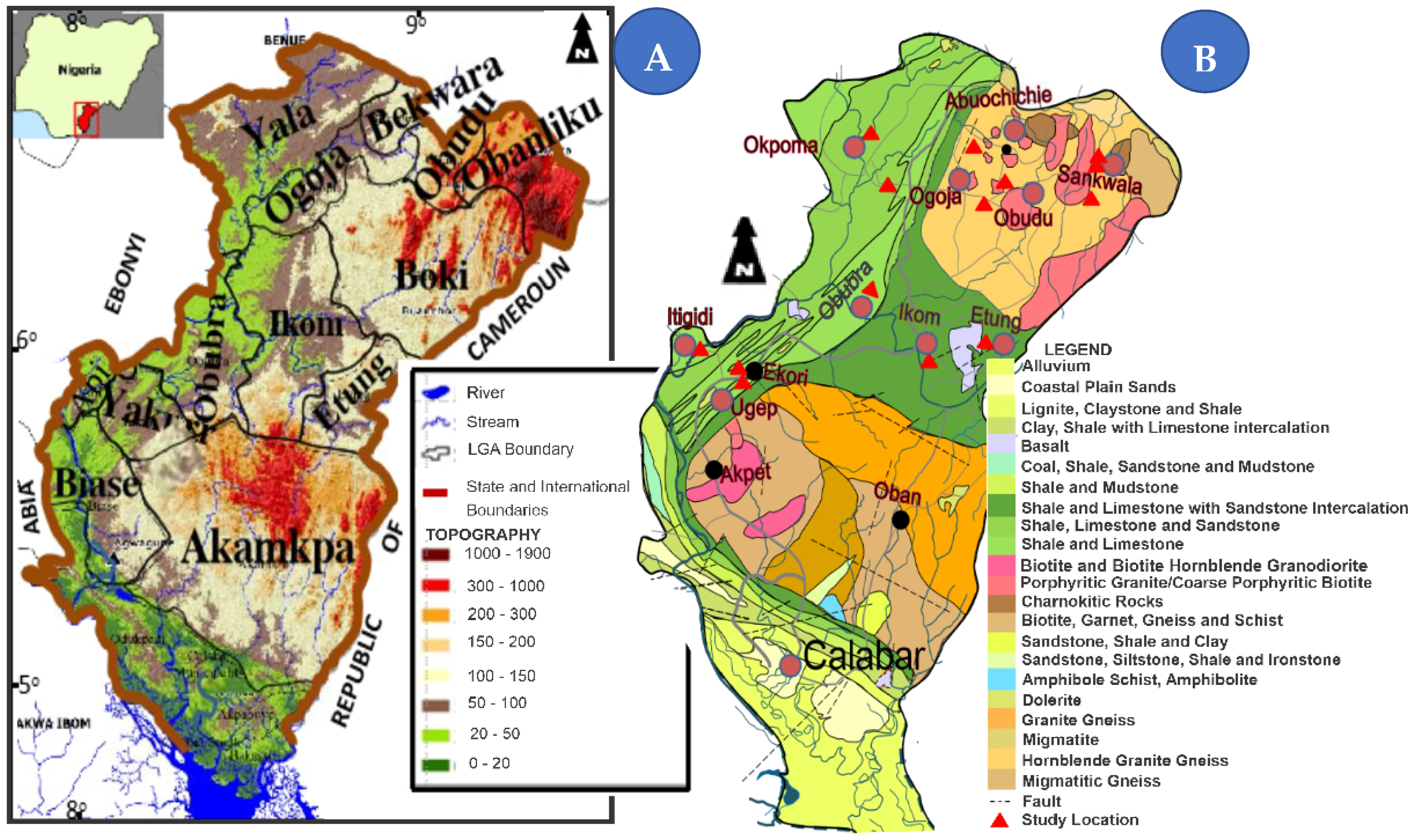
2.1. Physiographic Description of the Study Site

Cross River State (the study area) is located between longitudes 7°30′ and 9°30′ E of the Greenwich Meridian and latitudes 4°30′ and 7°00′ N of the Equator, in southeastern Nigeria. It shares its entire western boundary with the Republic of Cameroun, while Benue State in Central Nigeria occupies its northern margin. It is surrounded to the east by Abia, Akwa Ibom, and Ebonyi States, while the Atlantic Ocean and Akwa Ibom State border it to the south (Figure 1A). The investigation covers twelve local government areas (LGAs) (Figure 1A) located within the tropical rainforest belt of southern Nigeria. All the sites investigated are characterized by two distinct seasons, wet and dry, whose onset depends on the position of the intertropical convergence zone ITCZ (Figure 2) [30,31] that drives regional climatic conditions. When the ITCZ crosses the Equator into the Northern Hemisphere between March and mid-October, the moisture-laden trans-Atlantic wind blows inward from the Atlantic Ocean, resulting in heavy rainfall. However, when the ITCZ moves into the Southern Hemisphere between November and March, the predominantly dry and dusty trans-Saharan trade wind blows southward towards the coastal areas from the Sahara Desert. This period is usually characterized by rising temperature and aridity. The annual rainfall ranges from 1300 to 3000 mm, while temperatures and relative humidities are generally high throughout the year, averaging around 22.5 °C (i.e., 15–30 °C) and 88%, respectively. The peak period of the rainy season coincides with the period with the highest static water levels, surface runoffs, and humidity.
Furthermore, vast amounts of weakly cemented materials are usually dissolved, dislodged, transported (in both solution and suspension), and deposited in drains and river channels during the wet season. Their continuous action normally leaves the epithelial sediments perpetually dry and sandy, particularly where rock fragments are close to their provenance areas. Cross River State occupies a total area of 20,156 km2 and is drained by a network of rivers (with Cross, Kwa, and Munaya being the major ones), streams, and lakes. In the northern parts of the state, some of these water bodies are ephemeral. Rainfall is a major source of replenishment for both the surface and groundwater resources [32]. Sometimes, the percolating water transports substances in solution to the upper parts of the saturated aquifer, although the extent to which such substances reach the aquifer depends on the attenuating capacities of the overlying aquitards [33].

2.2. Geology and Hydrogeology

Cross River State sits on a complicated geological terrain comprising Precambrian Basement Complex (PBC) (dominated by the Precambrian Oban Massif and Obudu Plateau) and Cretaceous-Tertiary-Quaternary sediments (i.e., the Ikom-Manfe Embayment and Calabar Flank). Oban Massif and Obudu Plateau rocks are mostly high-grade metamorphic rocks that represent a westward extension of the Bamenda Massif in the Republic of Cameroun into the Cross River Plains in southeastern Nigeria. These rocks are widely dissected with a predominantly NW–SE trend in the Oban Massif and NE–SW direction with occasional N–S swing in the Obudu Plateau. Two major units comprising the ancient metasedimentary sequence, pre-Pan African (2.8 ± 1.3 Ga), and Pan African Older Granites PAOG (600 ± 1500 Ma) dominate the Precambrian terrain. Structural records on the rocks suggest that they have undergone polyphase deformation (resulting in their folding, faulting, foliation, and shearing) via Pan-African orogenic activities [34,35]. The rocks in the Obudu Plateau are dominated by high-temperature and pressure metamorphic rocks such as migmatites, gneisses, schists, amphibolites, cataclasites, and quartzites that have undergone amphibolite to granulite metamorphism [35]. The initial features of the rocks have been changed considerably by post-emplacement tectono-thermal and low-grade metamorphism [35,36,37]. The pre-Pan African rocks in the Oban Massif are dominated by migmatitic and sheared gneisses, para-ortho-schists, meta-conglomerates, and other ancient granitic rocks such as phyllites, while the Pan-African rocks consist mainly of older granites and metavolcanic sedimentary series [38,39]. The rocks are repeatedly intruded by rocks of acidic, intermediate, basic, and ultra-basic compositions such as charnockites, granitic plutons and pegmatites, aplites, quartz veins, and dolerite dykes [40].
The intra-continental Ikom-Mamfe Basin (IMB), a contiguous part of the Benue Trough (central Nigeria), is characterized by a low relief and undulating topography with elevations reaching ~300 m. The IMB is surrounded by comparatively higher geological terrain, including the northern Obudu Plateau (1716 m), southward Oban Massif (>1 km), and easterly Cameroun Mountain (>4 km). The Anambra Basin lies on its western boundary. The IMB is filled predominantly by a series of silicate mineral-enriched sediments of marine and terrestrial origin, including shales, sandstones, mudstones, limestones, and calcareous and carbonaceous rocks. The schists are quartz- and mica-enriched, while the gneissic rocks are feldspathic with textures varying from fine hornblende gneisses to black and white gneisses. These rocks strike dominantly in the E–W direction with occasional N–S swings. Petters et al. [41], and Ndip et al. [42] made a comprehensive documentation of the tectonic origin, depositional history, chemical composition, and depositional environment of rocks in the Ikom-Mamfe Embayment.
Post-Santonian tectonic disturbances resulted in younger granitic rocks such as syenites, diorites, trachytes, and basalts being emplaced in Cretaceous sediments, thereby distorting their physical, lithological, mechanical, chemical and structural states [43,44,45,46,47,48]. The sources of these magmatic activities have been traced to low-grade tectonic activities originating from the Cameroun Volcanic Line [49] and post-Santonian tectonic disturbances [50,51,52]. However, recent studies have shown that these disturbances did not reach parts of the Calabar Flank because the Guinea Ridge blocked their southward continuity [53,54,55]. The Cretaceous Calabar Flank (CF) is an epirogenic basin located between the southern margin of Oban Massif and the northeastern sector of the Tertiary Niger Delta in southeastern Nigeria. The basin is underlain by some dominantly northwest–southeast trending basement structures where the main tectonic elements include Ituk High (the epicenter of carbonate sedimentation) and Ikang Trough, the center of clastic sedimentation [43,44,45]. Lower-upper Cretaceous and Tertiary sediments comprising the Awi Sandstones, Mfamosing Limestones, Ekenkon and Nkporo Shales, New Netim Marls, and Benin Formation rest unconformably on the Precambrian basement. Petters et al. [45], Reyment [46], and Adeleye and Fayose [47] performed a detailed analysis of the lithological and chemical compositions of sediments in the CF, whose thickness is estimated to be about 3500 m [44].

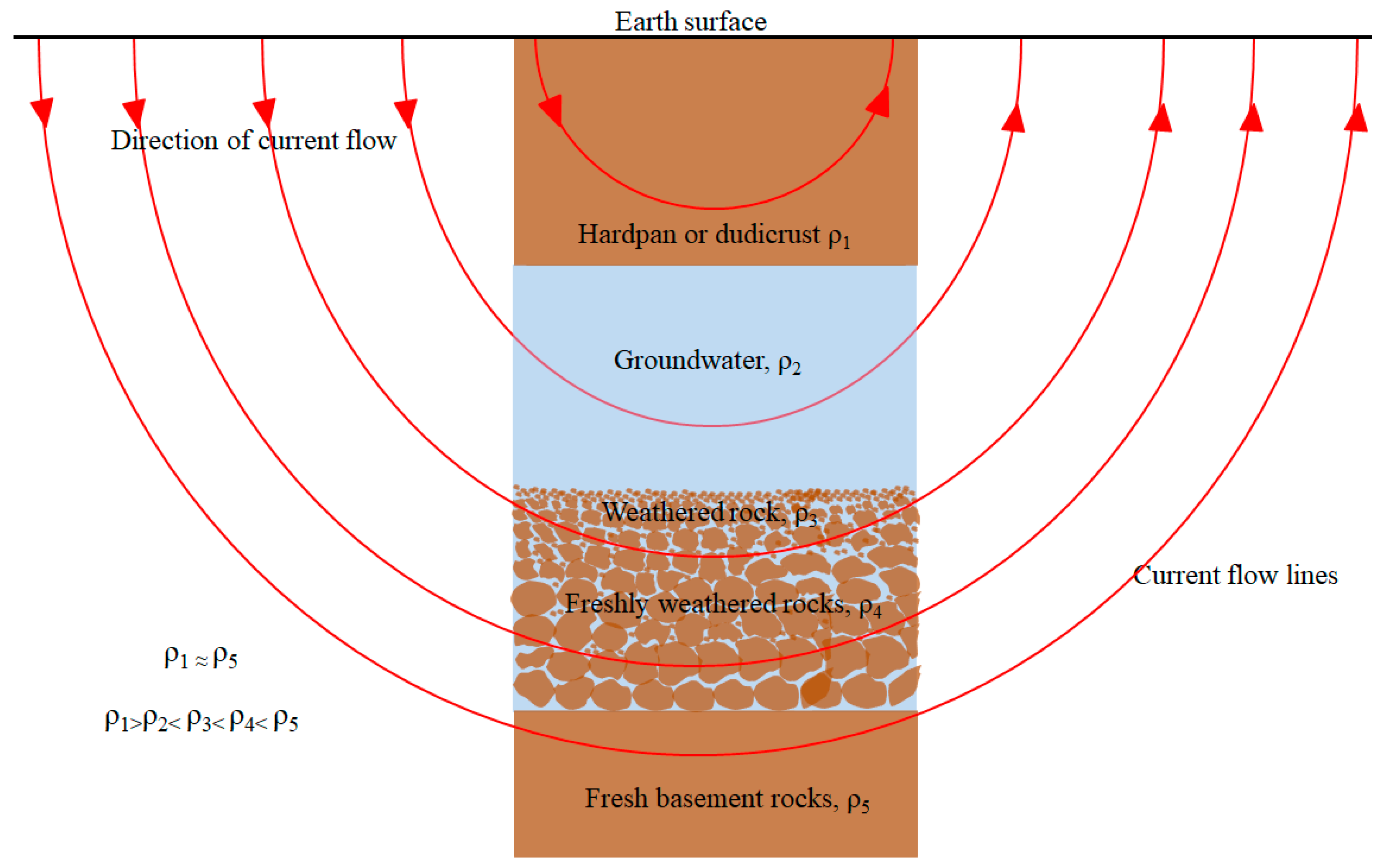
3. Aquifer Systems in the Study Area

Experimental studies have shown that hard rock aquifers in the study area—characterized by low (<1 L/s) to moderately high hydraulic permeability and storage capacity [28,56,57]—are highly anisotropic. The low permeability problems and their associated low groundwater yields are more pronounced in environments where the fractured materials are not interconnected. However, aquifers that are hydraulically connected to perennial or intermittent streams and buried river channels have enhanced transmissivities because of their continuous recharge [58]. Some researchers attributed the main source of recharge in the saprock aquifers to seepages from the overlying and adjourning regolith aquifers [59,60]. Fissuring and fracturing of rocks are usually more intense in the upper part of the rocks [61], thereby making this part more permeable than the basal parts.
A typical cross-sectional profile of a weathered hard-rock aquifer system consists of saprolitic and saprock aquifers [28]. These aquifer systems are capped by soils that vary from highly leached lateritic soils to angular soil horizons whose composition consists mainly of pisolitic laterites, quartz sands, and micas. The degree of weathering decreases vertically downwards until a hardpan (or duricrust) formed around the water table truncates their vertical continuity. The upper horizons of the saprolite are clayey unless leached, with gravel-like materials occurring at the basal parts of the main aquifer zone. Beyond this level, the porosity and permeability of the bedrock materials decrease rapidly with depth. In some locations, the effects of weathering extend more than 90 m below ground. These characteristics have been confirmed by many geochemical and pedological studies of deeply weathered profiles [61].
Weathered rock materials and finer particles transported in solution and suspension by groundwater exist inside a fracture. When these mixtures settle, they do so in columns based on their densities, with each column having unique electrical characteristics. If the various columns are suitably mapped, the upper groundwater-dominated layer can be identified directly from their high conductivities.

4. Data Acquisition

4.1. Vertical Electrical Sounding

The use of surface resistivity techniques for investigating the distribution and nature of subsurface materials and other environmental problems has been in practice for centuries, because of the dependence of rock resistivities on their physical parameters. The general procedure involves probing and monitoring the response of surficial materials to the passage of an impressed electric current flowing through them. Details of the theory and practical procedures can be found in Telford et al. [62], Zhdanov and Keller [63], and Keller and Frischknecht [64].
Field investigations involving geoelectrical surveys are usually performed using electrode configurations and field procedures of several types [62]. Schlumberger arrays, implemented using the vertical electrical sounding (VES) procedure, were adopted here because this study is focused on assessing vertical variations in subsurface resistivity. These VES investigations—conducted as part of broader consultancy services rendered to various water-drilling companies, student field trips, private borehole developers, and sponsored hydro-geophysical investigations between 2005 and 2021—were performed across different geological terrains and sites using different resistivity equipment, such as the SAS 300 and 1000 from ABEM (Sweden) and an SSP-ATS-MRP resistivity meter from IGIS (India). Some sites were occupied more than twice at different times with different equipment in some cases, and the same results were obtained. Current electrode spacings (AB) were site-dependent. In locations with fairly straight paths, the ABs were sometimes extended beyond 3000 m to permit the sampling of fairly deep-seated geological structures. The potential electrode separations (MNs) were fixed over a succession of measurement points before they were increased [65]. The MN increments were performed in conformity with the MN AB requirements [66]. Unfavorable field conditions such as settlement patterns, reserved areas, and topographic conditions constrained the profiles to be oriented along access roads to the areas and did not permit a repetition of the data acquisition in other directions. Contact resistance problems were adequately checked by pouring water and sometimes saltwater solutions at the electrode positions in locations where they were encountered.
Acquired data were plotted on bi-logarithmic graphs, from which the normal VES curves (Figure 3A) were identified and isolated from the abnormal ones (Figure 3B, Table 1). Satisfactory analyses of the unusual VES data were impossible because of the consistently high root-mean-square errors (>10%) observed between the modelled and measured data; hence, the data were interpreted qualitatively. Therefore, quantitative information such as layer thicknesses, depths, and layer resistivities (usually derived from the modelling of normal VES data) could not be determined.

4.2. Borehole Drilling and Pumping Tests

Drilling through the fissured-hard rocks was performed using the percussion rotary air blast (RAB) drilling technique, while the thin overburden materials were drilled using the rotary drilling method. The RAB uses a high-pressure compressed-air piston-driven hammer to energetically drive the drill bit into the hard rock formation. In each blow, rocks were crushed and the cuttings were blown to the surface by the rebounding compressed air. Cuttings blown to the surface were generally of low quality because they were contaminated by other rocks they contacted while being blown towards the surface. However, attempts were made to reconstruct the various lithologic units from samples blown to the surface (Figure 3C). Water is blown to the surface when the drill bit penetrates a saturated fracture, and severe air loss occurs when it penetrates its air-filled counterparts. The saturated fractures were usually encountered between 40 and 70 m.
The open wells were cased using high PVC casings. Slotted casings were used to screen the groundwater in the fractured regions. The slotted part of the borehole annulus was gravel-packed to further screen the groundwater, ensure the delivery of good quality water to the borehole, and stop the ingress of particles into the borehole. The boreholes were developed and grouted to prevent surface water flow into the well [67,68].
The wells were pump-tested to determine the yield of the aquifers and the optimal sizes of pumps to sustain their yields, using 24 h pumping and recovery data. The procedure involved measuring and recording static water levels inside boreholes before and after pumping. After pumping for a specific time, the drawdown levels were measured. The discharge rate was computed from the volume of the pumped water and analyzed. Under steady-state conditions, the transmissivity T was estimated from the pumping test data using Cooper-Jacob’s method [67], as
T = 2.303 Q 4 π Δ s
where Δ s is the change in drawdown over one log cycle (m). The typical graphs obtained are shown in Figure 3D. Equation (1) was considered suitable for determining T because the confining conditions varied from confined to semi-confined in most of the boreholes sampled. The acquired T data at the ten sites are shown in Table 1.

4.3. Lineament Density Map

A high-resolution 30 m ASTER (Advanced Space-borne Thermal Emission and Reflection Radiometer) procedure was adopted for mapping structures in the study area. The ASTER technique was adopted because of its capacity to generate enhanced-quality images, due to its improved spatial resolution. Generally, geomorphological characteristics such as ridges and valley alignments, mountain ridge relocations, scarp faces and watersheds, linear drainage channels, fractures in basement rocks, and continuities in surface depressions are commonly used when mapping linear features. However, in this study, the features of interest are those characterized by topographically negative lineaments that usually originate from fractures, faults, joints, and shear zones [69,70,71]. These linear geological structures comprising lineament frequency (Figure 4A) and lineament density (Figure 4B), as well as their main directions (Figure 4C), were mapped after contributions from non-geological features were eliminated [72].

5. Results and Discussion

Data acquired during VES investigations usually consist of those generated by responding crustal materials, which determine the trend of the VES curve, and some noisy components originating from a couple of extraneous sources (like galvanic distortions, system noise, near-surface changes in lithology, thin and suppressed layers, and so on). Distortions in the VES curve arising from extraneous sources like near-surface distortions caused by potential (P) and current (C) effects normally affect a segment of the VES curve [73]. This type of distortion always shifts a segment of the curve either above or below the normal trend of the VES curve relative to the apparent resistivity axes without altering its dominant trend. The noisy segments are usually identified by some isolated cases of some data plotting either above or below the dominant trend of the VES curve. Such disconnecting noisy data points are normally treated as outliers. Careful data management practices implemented during the data conversion, modelling and interpretational phases are normally adopted to either edit the affected data point (or segments) or completely delete (remove) them so long as such action will not compromise the data quality. Curve smoothening is one such data management practices usually performed to reduce noisy points or segments to their normal equivalent [72,73,74,75,76]. This procedure involves the careful removal of any outliers from the datasets to reduce their impacts, particularly on modelling and interpretational errors. A common assumption usually used as a guide while removing these outliers is that they carry no substantially useful subsurface information.
Some of the data acquired during the various data acquisition exercises have been documented and published elsewhere [27,28,29], and some citations therein. This category of VES data generated mainly KH, HK, KA, AH, HKH and KHK curve type (Figure 3A) while the groundwater table depths, which were site and geologic dependent, range between <5 and ~30 m [27,28,29]. The smoothened curves were free-flowing with an easily discernible trend. These curves depict the preponderance of shallow subsurface conditions with a heterogeneous and anisotropic distribution of materials. In locations where the capping materials are dominated by freshly weathered (coarse-textured and high-angularity) rock fragments due to their locations’ closeness to their provenance areas, apparent resistivities were generally high. Conversely, apparent resistivities were generally low at locations where argillaceous sediments dominate the shallow lithological sequence. The transition from one lithological unit to another is smooth indicating that the boundaries between the various modelled lithological units are not sharp but diffused. These groups of curves form the normal VES curves (Figure 3A) while those that deviate from this normal behavioural pattern constitute the abnormal curves (Figure 3B). The abnormal VES data were prevalent in the tectono-thermal environments and areas with vertical inhomogeneities.
The abnormal curves are characterized by some discontinuous segments caused by the presence of unusual data points and breaks in curve continuity. The irregular segments comprise some data points that either rise sharply or fall abruptly, sometimes forming cusp-like structures [77,78]. The formation of cusps and subsequent distortions in the VES curve trends have been attributed to many factors, including current leakage into the receiver unit [79]. The manifestation of such challenges in data acquired with the same equipment in other locations is supposed to serve as a confirmatory test for an outward source of this challenge. However, the persistence of these trend-distorting data points—even in data acquired at different times at a particular location, and sometimes using different equipment—rather points to a subterranean source. Furthermore, their unique signature of distorting VES curves only at specific points, and the ability of the curve to recover its distorted trend beyond that segment, differentiate them from those originating from non-subterranean sources such as galvanic and static distortions [73,80], near-surface heterogeneities, and noise from the measuring instrument [81,82].
Normal VES curves are usually free-flowing with no steep inclinations (>45°), because responding geological structures do not always dip (or incline) above (or below) 45o in normal environments [76,83,84]. Therefore, the unfamiliar plotting of some data points at 90o, which results in distortion of the trend of the curve, is indicative of the impacts of paleo-tectono-thermal disturbances in the rocks. This distortion degrades the free-flowing form of typical VES curves, thereby making them not only appear discontinuous but also deviate from the standard form of a multilayered VES curve. These peculiar curves were prevalent in the hard-rock-covered, tectonically disturbed, and low permeability metasedimentary areas (where younger rocks intrude into the overlying sediments in the Santonian, thereby creating subsurface unconformities and secondary porosities) [28]. This tectonic activity, coupled with the recurrent low-intensity metamorphic activities, stresses the rocks beyond their bearing capacities, leading to their deformation and the formation of unconformal geological structures (cracks, fractures, veins, faults, folds, pores, and so on) in the metasedimentary areas and fracturing in the basement areas. The intrusion of younger rocks into the overlying dominantly argillaceous sediments causes them to become domed, baked, fractured, and folded, forming anticlinal and synclinal structures [84,85,86] and thereby yielding secondary porosities. The origin, types, and characteristics of these structures, which serve as pathways controlling the hydrothermal mineralization intensity, localization, structure, character, and groundwater flow [48,50,87], are well-documented in relevant studies such as Morreau et al. [49], Verma and Bandyopadhyay [88], Stein et al. [89], Schultz and Fossen [90], Sibson et al. [91], and Suzuki et al. [92].
The lineaments/fractures, though more concentrated in the basement areas (Figure 3), are sparsely distributed in the low-permeability metasedimentary areas. Some fractures are long and intersect several times, indicating a dense network (0–13.5 km/km2) of interconnected pathways for groundwater storage and circulation. Lineaments in the metasedimentary areas such as Abuochichie, Ikom, Itigidi, Okpoma, Ogoja, and Ugep, where the original argillaceous sediments were forced to metamorphose into impervious shalestones, sandstones, siltstones, and claystones via tectonic activities, are short, isolated, and sparsely distributed. The recurrence of the low-scale tectonic activities resulted in the formation of impermeable geological structures such as hardpans, dudicrusts, and other unconformal secondary structures within sediments at some locations in the metasedimentary areas [93]. These unconformal structures exhibit unique electrical and petrophysical properties which—when suitably mapped—can be used to locate, identify, and model them as well as estimate their dimensions. In the metasedimentary regions, the number of these high-resistivity abnormal points is usually more than one. The total number of break-away points is indicative of the thickness, while their linear distribution above the trend of the curve is suggestive of the compactness of the unconformal structure. Thus, in the Ekori and Ekureku communities, where few points (five and three points, respectively) broke away, the unconformal structures are not very homogeneous. However, the unconformal structure observed in the Ijima community, with a high number of linearly distributed points, is thick and very homogeneous. These unconformal structures are underlain by comparatively low-resistivity materials. The resistivity values of the underlying materials increase gradually with depth until the curve recovers its interrupted trend in the basement areas. The unconformal structures do not exist in the basement regions because most fractures in this region are overlain by fissured materials and underlain by fresh basement in many locations. In these locations, one (or more) point(s) drop suddenly below the trend of the VES curve, such as in Amana, Okorshie, and Sankwala communities (Figure 3B, Table 1). This is indicative of a thin fracture where the fissured materials serve as the confining structure.
The unconformal structures are characterized by low permeability and porosity, and a higher resistivity relative to those of the adjoining materials [94]. These low-permeability structures serve as a trapping mechanism that blocks the continuous upward migration of fluids, including water vapor, thereby causing them to accumulate, become compressed, and later condense into groundwater below them when optimally compressed. The condensed groundwater dissolves materials within the fractures, leading to their sedimentation and segmentation into density- and gravity-induced layers within the fractures [95]. In the segmentation profile, the freshly weathered high-angularity rock fragments usually settle and occupy the base of the fracture, while finer particles that normally settle in suspension and solution in the groundwater usually occupy the upper water-filled top layer inside the fracture (Figure 5). When a reasonable volume of the groundwater accumulates at a particular point, topographic gradients usually cause them to start flowing out from the fractures.
The various lithological units, including the unconformal structures and the various settled layers within the fracture, possess unique physical properties which, if suitably mapped, can be used to isolate and identify them. The upper water-dominated top layer, characterized by a high electrical conductivity relative to those of the adjoining materials (including the unconformal structure and the basal rock-fragment-dominated materials) was aptly identified by the sudden drop in resistivity below the unconformal structure in the sedimentary areas and a sudden drop in resistivity values in the basement regions. Thus, groundwater accumulation below the unconformal high-resistivity structures was detected by the sudden drop in resistivity value, while those of other materials within the fracture were identified by the gradual recovery of resistivities below the water-dominated upper layer. Thus, a sudden drop in the apparent resistivity of materials below the unconformal high-resistivity structures is a direct indicator of groundwater accumulation below them, provided that the resistivity of the first dropped point is lower than those of the adjourning layers.
In well-developed and thick-apertured fractures, where more than one current flow line penetrates the fracture, the presence of conducting fluids (which is the main medium of electric current conduction) [96,97] will cause the first apparent resistivity to drop suddenly while the resistivity of other materials (corresponding to the response from other layers of materials penetrated by the subsequent current flow lines) will begin a gradual process of recovery by a stepwise increase in resistivity above that of the first suddenly dropped point. Attributing anomalously low resistivity observations to water-filled structures such as karst conduits, cavities, sinkholes, and fractures is a common interpretational practice in the electrical resistivity method. Zhu et al. [98] observed that a water-filled karst conduit mapped as an anomalous low-resistivity structure when successfully drilled will produce a high-yielding water pipe. Cheng et al. [99], while working in a complicated hydrogeological karst-dominated environment, attributed anomalously low-resistivity zones to saturated sinkholes and cavities. Hence, the abrupt drops in the resistivity values relative to those of the adjoining materials (unconformal structures in tectonically disturbed environments) are sometimes direct indicators of water saturation in fractures and cavities. Thus, with the compartmentalization of a water-filled fracture/cavity into layers by gravity-induced sedimentation, it becomes possible to map the upper water-dominated conducting layer based on its low-resistivity response compared to those of the adjoining materials. The electrical responses of the various layers in a fracture are such that the resistivities increase progressively with particle size, thereby giving the rock fragment-dominated basal layer the highest resistivities (Figure 5) [61,95]. Confirmatory results from the pump testing show that low-yielding fractures (<10 m3/day) manifest as a single abnormally dropped point. In comparison, if two or more anomalous data points drop consecutively, they indicate deeply weathered high-yielding fractures (>30 m3/day), provided that the resistivity of the first dropped point is less than those of the succeeding ones.
VES curves with a single anomalous break-point are indicative of poorly developed thin-apertured fractures that can only transmit small volumes of groundwater in unit time [99,100]. The single break-off point suggests that only one out of the eight current flow lines per decade penetrated the saturated zone. This type of fracture is thin and characterized by low transmissivity (<10 m3/day) (Figure 3, Table 1) and poor groundwater-yielding potential. This category of fracture is prevalent in locations with short and disconnected lineaments such as Abuochichie, Boki, Effraya, Itigidi, Ikom, Okpoma, Ogoja, Ugep, Sankwala, and Obudu (Figure 4A,B). In comparison, the long and densely interconnected fractures are common in locations where more points drop-off from the discernible trend of the VES curve. When two or more low-resistivity data points drop suddenly below the unconformal structure and/or trend of the VES curve, a thick-apertured fracture can be inferred. This implies that two or more successive current flow lines penetrated the saturated fracture over a decade. The aperture of this category of fracture is large enough to allow for the transmission of large volumes of water, provided that the resistivity of the first break-off point is lower than that of the succeeding break-off points. These fractures are characterized by high transmissivities and, consequently, better groundwater-yielding potential (Figure 4A, Table 1) [67,68]. The number of broken-off points below the unconformal structure/trend of the VES curve shows the number of conductive horizons within the fracture penetrated by the injected current [98,100,101]. The fidelity of the break-off points must be uniquely ascertained by implementing data quality management practices during data acquisition and processing. According to Day-Lewis et al. [102] and Tso et al. [102], the acquisition of high-fidelity data in the electrical resistivity method depends on many factors, including the sensitivity of the instrument used for data acquisition. Instrument sensitivity is a function that depends on the instrument’s capacity to maximally drive desired voltage into the ground [102,103]. Thus, both pre-field (e.g., measuring values of standard resistors and repeating and comparing measurements made at locations with known ground resistances) and in-situ (increasing the number of measuring points per decade, repeating measurements using the crossover technique and eliminating contact resistances) practices must be employed to confirm the reliability of the break-off point [102,103] before interpretation.
These findings contribute to ongoing efforts to directly identify groundwater accumulation zones in geologically complicated environments and economically estimate well performances (yield and water storage) from surficial data. The findings of this study, though limited to tectono-thermal areas, will be very useful in the search for a dependable technique for economically identifying productive fractures and estimating groundwater yield from surficial geophysical data. This is because geophysical techniques depend on the application of indirect procedures in extracting subsurface information, and such interpretational procedures consequently lack uniqueness because several sources can generate similar responses [104,105].

6. Conclusions

VES data acquired in tectono-thermally disturbed environments sometimes contain outliers when plotted on a bi-logarithmic graph. These noisy datasets usually distort the discernible trend of the VES curve, by plotting abnormally above or below its dominant trend at the point of their occurrence. This type of distortion is different from those arising from other causes such as galvanic and static distortions, which usually affect a segment of a curve without changing the curve’s trend. Allowing these unusual points to remain within the datasets during the data processing and modelling phases always produces unsatisfactory results because their presence usually causes the root-mean-square error to exceed the preset acceptable limit. Consequently, such data points are usually deleted to recover the trend of the curve and generate interpretable models during the traditional curve-smoothening (data processing) phase.
This study has shown that these unusual data points are indicative of groundwater accumulation zones in porous medium and can also estimate likely borehole productivities in tectono-thermally disturbed environments. A single-point drop signifies a low-yielding fracture characterized by small apertures. The groundwater yield from this group of fractures can barely support the daily domestic water needs of some families. However, VES curves where two or more points break away from the trend of the curve indicate high-yielding fractures or nonconformities, provided that the resistivity value of the first break-point is lower than those of subsequent ones. The productivity level of this category of fractures is high enough to support the water needs of families. The apparent resistivities of these saturated fractures usually vary between 40 and 500 Ωm, depending on the nature of the host rock. These qualitative interpretations have been confirmed by drilling and pumping test results. Depths to these water-filled fractures, though location-dependent, typically vary between 40 and 100 m in the study area. These saturated fractures are common in locations with high lineament density. Optimal data-quality-management practices—including determining the sensitivity level of the equipment, repeating the measuring process, and changing the potential electrode positions and, where possible, the VES profile orientation—must be implemented to confirm the integrity and subterranean nature of the break-off points.

Author Contributions

A.E.A., S.E.E. and U.C.B. applied formal analysis and data curation, supervised this work, and wrote the main manuscript. E.D.E., M.S.F., K.A., S.S.A., J.E.T., A.M.E. (Ahmed M. Eldosouky) and N.J.G. performed the investigation and prepared the figures. P.A. revised the manuscript. A.M.E. (Aniekan M. Ekanem) wrote, reviewed, and edited the main manuscript. All authors reviewed the manuscript. All authors have read and agreed to the published version of the manuscript.

Funding

This research was funded by the Researchers Supporting Project number RSP2024R351, King Saud University, Riyadh, Saudi Arabia.

Data Availability Statement

The data used in this study can be made available upon request to the authors.

Acknowledgments

The authors thank the support from the Researchers Supporting, King Saud University, Riyadh, Saudi Arabia.

Conflicts of Interest

The authors declare no conflict of interest.

References

  1. Giordano, M. Global groundwater? Issues and solutions. Annu. Rev. Environ. Resour. 2009, 34, 153–178. [Google Scholar] [CrossRef]
  2. Foster, S.; Chilton, J.; Nijsten, G.J.; Richts, A. Groundwater—A global focus on the ‘local resource’. Curr. Opin. Environ. Sustain. 2013, 5, 685–695. [Google Scholar] [CrossRef]
  3. Kearey, P.; Brooks, M.; Hill, I. An Introduction to Geophysical Exploration; Wiley-Blackwell: Hoboken, NJ, USA, 2002. [Google Scholar]
  4. Banks, D.; Nørmark, E.; Sørensen, K.I.; Skarphagen, H. Identifying the outflow of a deep thermal groundwater system in fractured crystalline bedrock using isotopic tracers and electrical conductivity. Appl. Geochem. 2008, 23, 1866–1878. [Google Scholar]
  5. Dewashushi, K.; Israil, M.; Mittal, S. Vertical electrical sounding to delineate fractures for groundwater in hard-rock terrain in the Siwana Ring Complex of Rajasthan, India. Environ. Geol. 2007, 52, 1523–1533. [Google Scholar]
  6. Biswas, A.; Sharma, S.P. (Eds.) Advances in Modeling and Interpretation in Near Surface Geophysics; Springer International Publishing: New York, NY, USA, 2020. [Google Scholar]
  7. Díaz-Alcaide, S.; Martínez-Santos, P. Advances in groundwater potential mapping. Hydrogeol. J. 2019, 27, 2307–2324. [Google Scholar] [CrossRef]
  8. Wyns, R.; Baltassat, J.M.; Lachassagne, P.; Legtchenko, A.; Vairon, J. Application of proton magnetic resonance soundings to groundwater reserves mapping in weathered basement rocks (Brittany, France). Bull. Société Géologique Fr. 2004, 175, 21–34. [Google Scholar] [CrossRef]
  9. Lachassagne, P.; Wyns, R.; Dewandel, B. The fracture permeability of hard rock aquifers is due neither to tectonics, nor to unloading, but to weathering processes. Terra Nova 2011, 23, 145–161. [Google Scholar] [CrossRef]
  10. Prowell, D.C. Cretaceous and Cenozoic tectonism on the Atlantic coastal margin. In The Geology of North America; Sheridan, R.E., Grow, J.A., Eds.; The Atlantic Continental Margin; Geological Society of America: Boulder, CO, USA, 1988; Chapter 29; Volume I-2, pp. 557–564. [Google Scholar]
  11. Mortimer, L.; Aydin, A.; Simmons, C.; Heinson, G.; Love, A.J. The role of in situ stress in determining hydraulic connectivity in a fractured rock aquifer (Australia). Hydrogeol. J. 2011, 19, 1293–1312. [Google Scholar] [CrossRef]
  12. Ofterdinger, U.; MacDonald, A.M.; Comte, J.C.; Young, M.E. Groundwater in fractured bedrock environments: Managing catchment and subsurface resources—An introduction. Geol. Soc. Lond. Spec. Publ. 2019, 479, 1–9. [Google Scholar] [CrossRef]
  13. Singhal BB, S.; Gupta, R.P. Applied Hydrogeology of Fractured Rocks; Kluwer Academic: Dordrecht, The Netherlands, 1999. [Google Scholar]
  14. Balasubramanian, A. Methods of Grounddwater Exploration; Centre for Advanced Studies in Earth Science, University of Mysore: Nanaimo, BC, Canada, 2007; p. 13. [Google Scholar]
  15. MacDonald, A.; Bonsor, H.C.; Dochartaigh, B.E.; Taylor, R.G. Quantitative maps of groundwater resources in Africa. Environ. Res. Lett. 2012, 7, 024009. [Google Scholar] [CrossRef]
  16. Maurice, L.; Taylor, R.G.; Tindimugaya, C.; MacDonald, A.M.; Johnson, P.; Kaponda, A.; Owor, M.; Sanga, H.; Bonsor, H.C.; Darling, W.G.; et al. Characteristics of high-intensity groundwater abstractions from weathered crystalline bedrock aquifers in East Africa. Hydrogeol. J. 2019, 27, 459–474. [Google Scholar] [CrossRef]
  17. Earon, R.; Dehkordi, S.E.; Olofsson, B. Groundwater Resources Potential in Hard Rock Terrain: A Multivariate Approach. Groundwater 2015, 53, 748–758. [Google Scholar] [CrossRef] [PubMed]
  18. Wright, E.P. The hydrogeology of crystalline basement aquifers in Africa. In The Hydrogeology of Crystalline Basement Aquifers in Africa; Wright, E.P., Burgess, W.G., Eds.; Geological Society, Special Publications: London, UK, 1992; Volume 66, pp. 1–27. [Google Scholar]
  19. Goldman, M.; Neubauer, F.M. Groundwater Exploration using Integrated Geophysical Techniques. Surv. Geophys. 1994, 15, 331–361. [Google Scholar] [CrossRef]
  20. Srivastava, P.K.; Bhattacharya, A.K. Groundwater assessment through an integrated approach using remote sensing, GIS and resistivity techniques: A case study from a hard rock terrain. Int. J. Remote Sens. 2006, 27, 4599–4620. [Google Scholar] [CrossRef]
  21. Pride, S.R. Relationships between seismic and hydrological properties. Hydrogeophysics 2005, 50, 253–290. [Google Scholar]
  22. Yaramanci, U.; Lange, G.; Knödel, K. Surface NMR within a combined geophysical survey in Haldenslaben (Germany). Geophys. Prospect. 1999, 47, 923–943. [Google Scholar] [CrossRef]
  23. Zaresefat, M.; Derakhshani, R.; Nikpeyman, V.; GhasemiNejad, A.; Raoof, A. Using artificial intelligence to identify suitable artificial groundwater recharge areas for the Iranshahr basin. Water 2023, 15, 1182. [Google Scholar] [CrossRef]
  24. Agrawal, P.; Sinha, A.; Kumar, S.; Agarwal, A.; Banerjee, A.; Villuri, V.G.K.; Annavarapu, C.S.R.; Dwivedi, R.; Dera, V.V.R.; Sinha, J.; et al. Exploring artificial intelligence techniques for groundwater quality assessment. Water 2021, 13, 1172. [Google Scholar] [CrossRef]
  25. Ernstson, K.; Kirsch, R. Geoelectrical methods. In Groundwater Geophysics: A Tool for Hydrogeology; Springer: Berlin/Heldelberg, Germany, 2006; pp. 84–117. [Google Scholar]
  26. Akpan, A.E.; Ugbaja, A.N.; George, N.J. Integrated geophysical, geochemical and hydrogeological investigation of shallow groundwater resources in parts of the Ikom-Mamfe Embayment and the adjoining areas in Cross River State, Nigeria. Environ. Earth Sci. 2013, 70, 1435–1456. [Google Scholar] [CrossRef]
  27. Ebong, E.D.; Akpan, A.E.; Emeka, C.N.; Urang, J.G. Groundwater quality assessment using geoelectrical and geochemical approaches: Case study of Abi area, southeastern, Nigeria. Appl. Water Sci. 2017, 7, 2463–2478. [Google Scholar] [CrossRef]
  28. Akpan, A.E.; Ebong, E.D.; Ekwok, S.E. Assessment of the state of soils, shallow sediments and groundwater salinity in Abi, Cross River State, Nigeria. Environ. Earth Sci. 2015, 73, 8547–8563. [Google Scholar] [CrossRef]
  29. Nicholson, S.E. The ITCZ and the seasonal cycle over equatorial Africa. Bull. Am. Meteorol. Soc. 2018, 99, 337–348. [Google Scholar] [CrossRef]
  30. Doherty, O.M.; Riemer, N.; Hameed, S. Role of the convergence zone over West Africa in controlling Saharan mineral dust load and transport in the boreal summer. Tellus B Chem. Phys. Meteorol. 2014, 66, 23191. [Google Scholar] [CrossRef]
  31. Edet, A.; Worden, R.H. Monitoring of the physical parameters and evaluation of the chemical composition of river and groundwater in Calabar (Southeastern Nigeria). Environ. Monit. Assess. 2009, 157, 243–258. [Google Scholar] [CrossRef] [PubMed]
  32. Ekanem, A.M.; Akpan, A.E.; George, N.J.; Thomas, J.E. Appraisal of protectivity and corrosivity of surficial hydrogeological units via geo-sounding measurements. Environ. Monit. Assess. 2021, 193, 1–22. [Google Scholar] [CrossRef]
  33. Ajibade, A.C.; Fitches, W.R. The Nigerian Precambrian and the Pan-African Orogeny. In Precambrian Geology of Nigeria; Oluyide, P.O., Mbonu, W.C., Ogezi, A.E.O., Egbuniwe, I.G., Ajibade, A.C., Umeji, A.C., Eds.; Geological Survey of Nigeria: Lagos, Nigeria, 1988; Volume 1, pp. 43–45. [Google Scholar]
  34. Hamimi, Z.; Eldosouky, A.M.; Hagag, W.; Kamh, S.Z. Large-scale geological structures of the Egyptian Nubian Shield. Sci. Rep. 2023, 13, 1923. [Google Scholar] [CrossRef]
  35. Ukaegbu, V.U.; Beka, F.T. Petrochemistry and geotectonic significance of enderbite-charnockit association in the Pan-African Obudu plateau, southeastern Nigeria. J. Min. Geol. 2007, 43, 1–14. [Google Scholar]
  36. Eseme, E.; Agyingi, C.M.; Foba-Tendo, J. Geochemistry and genesis of brine emanations from Cretaceous strata of the Mamfe Basin, Cameroon. J. Afr. Earth Sci. 2002, 35, 467–476. [Google Scholar] [CrossRef]
  37. Rahman, M.A.; Ukpong, E.E.S.; Azmatullah, M. Geology of Parts of the Oban Massif Southeastern Nigeria. J. Min. Geol. 1981, 18, 60–65. [Google Scholar]
  38. Ekwueme, B.N. Rb-Sr age and petrologic features of the Precambrian rocks from Oban Massif southeastern Nigeria. Precambrian Res. 1990, 47, 271–286. [Google Scholar] [CrossRef]
  39. Ukaegbu, V.U.; Ekwueme, B.N. Petrogenesis and geotectonic setting of the Pan-African basement rocks in Bamenda Massif, Obudu Plateau, southeastern Nigeria: Evidence from trace element geochemistry. Chin. J. Geochem. 2006, 25, 122–131. [Google Scholar] [CrossRef]
  40. Petters, S.W.; Okereke, C.S.; Nwajide, C.S. Geology of the Mamfe Rift, south eastern Nigeria. In Current Research in African Earth Sciences; Mathesis, G., Shandemerer, J., Eds.; Balkema: Rotterdam, The Netherlands, 1987; pp. 299–302. [Google Scholar]
  41. Ndip, E.Y.; Agyingyi, C.M.; Nton, M.E.; Oladunjoye, M.A. Review of the geology of Mamfe sedimentary basin, SW Cameroon, Central Africa. J. Oil Gas Petrochem. Sci. 2018, 1, 35–40. [Google Scholar] [CrossRef]
  42. Ekwueme, B.N. The chemical composition and industrial quality of limestones and marls on the Calabar Flank, southeastern Nigeria. J. Min. Geol. 1985, 22, 51–56. [Google Scholar]
  43. Reijers, T.J.A.; Petters, S.W. Depositional environments and diagenesis of Albian carbonates on the Calabar Flank, SE Nigeria. J. Pet. Geol. 1987, 10, 283–294. [Google Scholar] [CrossRef]
  44. Petters, S.W.; Nyong, E.E.; Akpan, E.B.; Essien, N.U. Lithostratigraphic revision for the Calabar Flank, SE Nigeria. In Proceedings of the 31st Anniversary Conference of Nigeria Mining and Geosciences Society, Calabar, Nigeria, 15–17 March 1995; Planets Space. Volume 57, pp. 755–760. [Google Scholar]
  45. Reyment, R.A. Aspects of the Geology of Nigeria: The Stratigraphy of the Cretaceous and Cenozoic Deposits; University Press: Ibadan, Nigeria, 1965. [Google Scholar]
  46. Adeleye, D.R.; Fayose, F.A. Stratigraphy of the type section of Awi Formation, Odukpani area, Southern Nigeria. J. Min. Geol. 1978, 15, 33–57. [Google Scholar]
  47. Ekwok, S.E.; Akpan, A.E.; Ebong, E.D. Enhancement and modelling of aeromagnetic data of some inland basins, southeastern Nigeria. J. Afr. Earth Sci. 2019, 155, 43–53. [Google Scholar] [CrossRef]
  48. Morreau, C.; Regnoult, J.M.; Deruelle, B.; Robineau, B. A new tectonic model for the Cameroon Line, Central Africa. Tectonophysics 1987, 139, 317–334. [Google Scholar] [CrossRef]
  49. Benkhelil, J. Cretaceous deformation, magmatism, and metamorphism in the Lower Benue Trough, Nigeria. Geol. J. 1987, 22, 467–493. [Google Scholar] [CrossRef]
  50. Burke, K.C.; Dessauvagie TJ, F.; Whiteman, A.W. Geological history of the Benue Valley and adjacent areas. In African Geology; University of Ibadan Press: Ibadan, Nigeria, 1972; pp. 187–206. [Google Scholar]
  51. Agagu, O.K.; Adighije, C.I. Tectonic and sedimentation framework of the lower Benue Trough, southeastern Nigeria. J. Afr. Earth Sci. 1983, 1, 267–274. [Google Scholar] [CrossRef]
  52. Ekwok, S.E.; Akpan, A.E.; Achadu OI, M.; Ulem, C.A. Implications of tectonic anomalies from potential field data in some parts of Southeast Nigeria. Environ. Earth Sci. 2022, 81, 1–15. [Google Scholar] [CrossRef]
  53. Mascle, J.; Blarez, E.; Marinho, M. The shallow structures of the Guinea and Ivory Coast-Ghana transform margins: Their bearing on the Equatorial Atlantic Mesozoic evolution. Tectonophysics 1988, 155, 193–209. [Google Scholar] [CrossRef]
  54. Fairhead, J.D. Mesozoic plate tectonic reconstructions of the central South Atlantic Ocean: The role of the West and Central African rift system. Tectonophysics 1988, 155, 181–191. [Google Scholar] [CrossRef]
  55. Okereke, C.S.; Esu, E.O.; Edet, A.E. Determination of potential groundwater sites using geological and geophysical techniques in the Cross River State, southeastern Nigeria. J. Afr. Earth Sci. 1998, 27, 149–163. [Google Scholar] [CrossRef]
  56. Edet, A.E.; Okereke, C.S. Assessment of hydrogeological conditions in basement aquifers of the Precambrian Oban massif, southeastern Nigeria. J. Appl. Geophys. 1997, 36, 195–204. [Google Scholar] [CrossRef]
  57. Titus, R.; Beekman, H.; Adams, S.; Strachan, L. The Basement Aquifers of Southern Africa; Report No. TT, 428-09; Water Research Commission: Pretoria, South Africa, 2009. [Google Scholar]
  58. Owoade, A. The potential for minimising drawdowns in groundwater wells in tropical aquifers. J. Afr. Earth Sci. 1995, 20, 289–293. [Google Scholar] [CrossRef]
  59. Dewandel, B.; Lachassagne, P.; Wyns, R.; Maréchal, J.C.; Krishnamurthy, N.S. A generalised 3-D geological and hydrogeological conceptual model of granite aquifers controlled by single or multiphase weathering. J. Hydrol. 2006, 330, 260–284. [Google Scholar] [CrossRef]
  60. Elster, D.; Holman, I.P.; Parker, A.; Ridge, L. An investigation of the basement complex aquifer system in Lofa county, Liberia, for the purpose of siting boreholes. Q. J. Eng. Geol. Hydrogeol. 2014, 47, 159–167. [Google Scholar] [CrossRef]
  61. Telford, W.M.; Telford, W.M.; Geldart, L.P.; Sheriff, R.E. Applied Geophysics, 2nd ed.; Cambridge University Press: Cambridge, UK, 1990; p. 732. [Google Scholar]
  62. Zhdanov, M.S.; Keller, G.V. The geoelectrical methods in geophysical exploration. Methods Geochem. Geophys. 1994, 31, 873. [Google Scholar]
  63. Keller, G.V.; Frischknecht, F.C. Electrical Methods in Geophysical Prospecting; Pergamon Press Inc.: Oxford, UK, 1966. [Google Scholar]
  64. Osman, M.M.; El-Qady, G.M.; Abdel Fattah, T.; Rashed, M.; Mohamdeen, M. Enhancement the VES models based on the TEM measurements and the application of static shift corrections.: Case study from Egypt. NRIAG J. Astron. Geophys. 2021, 10, 279–289. [Google Scholar] [CrossRef]
  65. Gowd, S.S. Electrical resistivity surveys to delineate groundwater potential aquifers in Peddavanka watershed, Anantapur District, Andhra Pradesh, India. Environ. Geol. 2004, 46, 118–131. [Google Scholar] [CrossRef]
  66. Freeze, R.A.; Cherry, J.A. Groundwater; Prentice-Hall: Upper Saddle River, NJ, USA, 1979; p. 604. [Google Scholar]
  67. Younger, P.L. Groundwater in the Environment: An Introduction; Blackwell Publishing: Hoboken, NJ, USA, 2007; p. 318. [Google Scholar]
  68. Solomon, S.; Ghebreab, W. Lineament characterisation and their tectonic significance using Landsat TM data and field studies in the central highlands of Eritrea. J. Afr. Earth Sci. 2006, 46, 371–378. [Google Scholar] [CrossRef]
  69. Akram, M.S.; Mirza, K.; Zeeshan, M.; Ali, I. Correlation of Tectonics with Geologic Lineaments Interpreted from Remote Sensing Data for Kandiah Valley, Khyber-Pakhtunkhwa, Pakistan. J. Geol. Soc. India 2019, 93, 607–613. [Google Scholar] [CrossRef]
  70. Elmahdy, S.I.; Mohamed, M.M.; Ali, T.A. Automated detection of lineaments express geological linear features of a tropical region using topographic fabric grain algorithm and the SRTM DEM. Geocarto Int. 2021, 36, 76–95. [Google Scholar] [CrossRef]
  71. Yassaghi, A. Integration of Landsat imagery interpretation and geomagnetic data on verification of deep-seated transverse fault lineaments in SE Zagrosa, Iran. Int. J. Remote Sens. 2006, 27, 4529–4544. [Google Scholar] [CrossRef]
  72. Ritz, M.; Robain, H.; Pervago, E.; Albouy, Y.; Camerlynck, C.; Descoitres, M.; Mariko, A. Improvement to resistivity pseudosection modelling by removal of near-surface inhomogeneity effects: Application to a soil system in south Cameroon. Geophys. Prospect. 1999, 47, 85–101. [Google Scholar] [CrossRef]
  73. Abdulkadir, Y.A.; Fisseha, S. Mapping the spatial variability of subsurface resistivity by using vertical electrical sounding data and geostatistical analysis at Borena Area, Ethiopia. MethodsX 2022, 9, 101792. [Google Scholar] [CrossRef]
  74. Makrini, S.E.; Boualoul, M.; Mamouch, Y.; El Makrini, H.; Allaoui, A.; Randazzo, G.; Roubil, A.; El Hafyani, M.; Lanza, S.; Muzirafuti, A. Vertical Electrical Sounding (VES) Technique to Map Potential Aquifers of the Guigou Plain (Middle Atlas, Morocco): Hydrogeological Implications. Appl. Sci. 2022, 12, 12829. [Google Scholar] [CrossRef]
  75. Key, K.; Constable, S. Coast effect distortion of marine magnetotelluric data: Insights from a pilot study offshore northeastern Japan. Phys. Earth Planet. Inter. 2011, 184, 194–207. [Google Scholar] [CrossRef]
  76. Gaber, A.; Mohamed, A.K.; ElGalladi, A.; Abdelkareem, M.; Beshr, A.M.; Koch, M. Mapping the groundwater potentiality of West Qena Area, Egypt, using integrated remote sensing and hydro-geophysical techniques. Remote Sens. 2020, 12, 1559. [Google Scholar] [CrossRef]
  77. Zohdy, A.A.R.; Eaton, G.P.; Mabey, D.R. Application of Surface Geophysics to Ground-Water Investigations (No. 02-D1); US Geological Survey Professional Paper; United States Geological Survey: Reston, Virginia, USA, 1974; 600-D. Available online: https://pubs.usgs.gov/twri/twri2-d1/pdf/twri_2-D1_b.pdf (accessed on 7 November 2023).
  78. Mlangi, T.M.; Mulibo, G.D. Delineation of shallow stratigraphy and aquifer formation at Kahe Basin, Tanzania: Implication for potential aquiferous formation. J. Geosci. Environ. Prot. 2018, 6, 78–98. [Google Scholar] [CrossRef]
  79. Meju, M.A. Joint inversion of TEM and distorted MT soundings: Some effective practical considerations. Geophysics 1996, 61, 56–65. [Google Scholar] [CrossRef]
  80. Gallardo, L.A.; Meju, M.A. Characterization of heterogeneous near-surface materials by joint 2D inversion of dc resistivity and seismic data. Geophys. Res. Lett. 2003, 30, 1658. [Google Scholar] [CrossRef]
  81. Sasaki, Y.; Meju, M.A. Three-dimensional joint inversion for magnetotelluric resistivity and static shift distributions in complex media. J. Geophys. Res. Solid Earth 2006, 111. [Google Scholar] [CrossRef]
  82. Cerri, R.I.; Reis, F.A.; Gramani, M.F.; Giordano, L.C.; Zaine, J.E. Landslides Zonation Hazard: Relation between geological structures and landslides occurrence in hilly tropical regions of Brazil. An. Acad. Bras. Ciências 2017, 89, 2609–2623. [Google Scholar] [CrossRef] [PubMed]
  83. Ejiga, E.G.; Ismail NE, H.; Yusoff, I. Implementing Digital Edge Enhancers on Improved High-Resolution Aeromagnetic Signals for Structural-Depth Analysis around the Middle Benue Trough, Nigeria. Minerals 2021, 11, 1247. [Google Scholar] [CrossRef]
  84. Song, Y.; Ren, J.; Stepashko, A.A.; Li, J. Post-rift geodynamics of the Songliao Basin, NE China: Origin and significance of T11 (Coniacian) unconformity. Tectonophysics 2014, 634, 1–18. [Google Scholar] [CrossRef]
  85. Song, G.; Wang, H.; Gan, H.; Sun, Z.; Liu, X.; Xu, M.; Ren, J.; Sun, M.; Sun, D. Paleogene tectonic evolution controls on sequence stratigraphic patterns in the central part of deepwater area of Qiongdongnan Basin, northern South China Sea. J. Earth Sci. 2014, 25, 275–288. [Google Scholar] [CrossRef]
  86. Birdsell, D.T.; Rajaram, H.; Dempsey, D.; Viswanathan, H.S. Hydraulic fracturing fluid migration in the subsurface: A review and expanded modeling results. Water Resour. Res. 2015, 51, 7159–7188. [Google Scholar] [CrossRef]
  87. Verma, R.K.; Bandyopadhyay, T.K. Use of the resistivity method in geological mapping—Case histories from Raniganj Coalfield, India. Geophys. Prospect. 1983, 31, 490–507. [Google Scholar] [CrossRef]
  88. Stein, R.S.; King, G.C.; Rundle, J.B. The growth of geological structures by repeated earthquakes 2. Field examples of continental dip-slip faults. J. Geophys. Res. Solid Earth 1988, 93, 13319–13331. [Google Scholar] [CrossRef]
  89. Schultz, R.A.; Fossen, H. Terminology for structural discontinuities. AAPG Bull. 2008, 92, 853–867. [Google Scholar] [CrossRef]
  90. Sibson, R.H.; Robert, F.; Poulsen, K.H. High-angle reverse faults, fluid-pressure cycling, and mesothermal gold-quartz deposits. Geology 1988, 16, 551–555. [Google Scholar] [CrossRef]
  91. Suzuki, K.; Toda, S.; Kusunoki, K.; Fujimitsu, Y.; Mogi, T.; Jomori, A. Case studies of electrical and electromagnetic methods applied to mapping active faults beneath the thick Quaternary. In Developments in Geotechnical Engineering; Elsevier: Amsterdam, The Netherlands, 2000; Volume 84, pp. 29–45. [Google Scholar]
  92. Rammlmair, D. Hard pan formation on mining residuals. In Uranium in the Aquatic Environment; Springer: Berlin/Heidelberg, Germany, 2002; pp. 173–182. [Google Scholar]
  93. Nicchio, M.A.; Balsamo, F.; Nogueira FC, C.; Aldega, L.; Pontes CC, C.; Bezerra, F.H.; de Souza, J.A.B. The effect of fault-induced compaction on petrophysical properties of deformation bands in poorly lithified sandstones. J. Struct. Geol. 2023, 166, 104758. [Google Scholar] [CrossRef]
  94. Cardona, A.; Finkbeiner, T.; Santamarina, J.C. Natural rock fractures: From aperture to fluid flow. Rock Mech. Rock Eng. 2021, 54, 5827–5844. [Google Scholar] [CrossRef]
  95. Yolcubal, I.; Brusseau, M.L.; Artiola, J.F.; Wierenga, P.; Wilson, L.G. Environmental physical properties and processes. In Environmental Monitoring and Characterization; Artiola, J., Pepper, I.L., Brusseau, M.L., Eds.; Academic Press: Cambridge, MA, USA, 2004; pp. 207–239. [Google Scholar]
  96. Steelman, C.M.; Kennedy, C.S.; Capes, D.C.; Parker, B.L. Electrical resistivity dynamics beneath a fractured sedimentary bedrock riverbed in response to temperature and groundwater–surface water exchange. Hydrol. Earth Syst. Sci. 2017, 21, 3105–3123. [Google Scholar] [CrossRef]
  97. Zhu, J.; Currens, J.C.; Dinger, J.S. Challenges of using electrical resistivity method to locate karst conduits—A field case in the Inner Bluegrass Region, Kentucky. J. Appl. Geophys. 2011, 75, 523–530. [Google Scholar] [CrossRef]
  98. Cheng, Q.; Chen, X.; Tao, M.; Binley, A. Characterization of karst structures using quasi-3D electrical resistivity tomography. Environ. Earth Sci. 2019, 78, 1–12. [Google Scholar] [CrossRef]
  99. Zou, L.; Håkansson, U.; Cvetkovic, V. Yield-power-law fluid propagation in water-saturated fracture networks with application to rock grouting. Tunn. Undergr. Space Technol. 2020, 95, 103170. [Google Scholar] [CrossRef]
  100. Zhang, W.C.; He, L.; Li, H.J.; Meng, Y.L.; Yang, F.B. Genesis and distribution of secondary porosity in the deep horizon of Gaoliu area, Nanpu Sag. Pet. Explor. Dev. 2008, 35, 308–312. [Google Scholar] [CrossRef]
  101. Day-Lewis, F.D.; Johnson, C.D.; Singha, K.; Lane, J.W.J. Best Practices in Electrical Resistivity Imaging: Data Collection and Processing, and Application to Data from Corinna, Maine; EPA Report: Boston, MA, USA, 2008. [Google Scholar]
  102. Foti, S.; Comina, C.; Boiero, D.; Socco, L.V. Non-uniqueness in surface-wave inversion and consequences on seismic site response analyses. Soil Dyn. Earthq. Eng. 2009, 29, 982–993. [Google Scholar] [CrossRef]
  103. Tso CH, M.; Kuras, O.; Wilkinson, P.B.; Uhlemann, S.; Chambers, J.E.; Meldrum, P.I.; Graham, J.; Sherlock, E.F.; Binley, A. Improved characterisation and modelling of measurement errors in electrical resistivity tomography (ERT) surveys. J. Appl. Geophys. 2017, 146, 103–119. [Google Scholar] [CrossRef]
  104. Güdük, N.; De La Varga, M.; Kaukolinna, J.; Wellmann, F. Model-based probabilistic inversion using magnetic data: A case study on the Kevitsa deposit. Geosciences 2021, 11, 150. [Google Scholar] [CrossRef]
  105. Colombo, D.; Turkoglu, E.; Li, W.; Rovetta, D. Coupled physics-deep learning inversion. Comput. Geosci. 2021, 157, 104917. [Google Scholar] [CrossRef]
Figure 1. (A) Topography and (B) generalized geological maps of Cross River State (Nigeria), showing some sampling locations. Insert in subfigure (A): map of Nigeria, showing the location of Cross River State.
Water 15 03946 g001
Figure 2. Movement of the Intertropical Convergence Zone over the African Continent in (A) wet season and (B) dry season.
Water 15 03946 g002
Figure 3. Graphical presentation of some normal VES curves (A) generated from parts of the 12 LGAs. Samples of some abnormal VES curves and their respective pumping test results generated from Amana (Bi and Di) and Okorshie (Bii and Dii) in Obudu LGA; Sankwala (Biii and Diii) in Obanliku LGA, Ekori (Biv and Div) and Ijima (Bv and Dv) in Yakurr LGA; and Ekureku (Bvi and Dvi) in Abi LGA. Insert: Descriptions of the lithologic log and graphs (C).
Water 15 03946 g003aWater 15 03946 g003b
Figure 4. Lineament density maps of Cross River State in (A) contoured and (B) isolated formats. (C) A Ross diagram showing the main direction of the lineaments.
Water 15 03946 g004
Figure 5. Schematic diagram of the distribution of materials inside a fracture.
Water 15 03946 g005
Table 1. Summary of anomalous data points and their locations.
S/No.Name of CommunityLocal Government AreaLocal GeologyAB/2 (m) at Breaking Point(s)Number of Points that Break-offApparent Resistivities at Breaking Point(s) (Ωm)Transmissivity (m3/day)
MinimumMaximumMinimumMaximum
1AkamkpaAkamkpaBasement60.060.01155.3-6.17
2KukareObanlikuBasement50.050.01120.57-6.24
3AmanaObanlikuBasement20.020.0196.59-8.99
4AmungaObanlikuBasement60.060.01210.05-5.99
5BayagaObanlikuBasement100.0aaaagok1405.35-8.52
6SankwalaObanlikuBasement30.030.01205.12-5.99
7MbenegeObuduBasement100.0150.01115.72-15.20
8BendigieObanlikuBasement80.0100.02529.98531.887.51
9OkorshieObuduBasement60.080.02120.00625.0032.12
10ObuduObuduBasement30.0150.0>2332.00457.0038.21
11EkoriYakurrMetasedimentary40.0250.0>287.96132.5452.21
12IjimaYakurrMetasedimentary150.0250.0>2126.26183.6054.29
13EkurekuAbiMetasedimentary15–20100–150>2588.59–978.391827.45–2487.1545.37
14AbachorYalaMetasedimentary30.0250.0>2110.20162.0651.04
15WulaBokiBasement50–60150.0>2330.32–628.08182.6343.12
16UtugwangObuduBasement100.0200.0>2127.61492.9541.20
Disclaimer/Publisher’s Note: The statements, opinions and data contained in all publications are solely those of the individual author(s) and contributor(s) and not of MDPI and/or the editor(s). MDPI and/or the editor(s) disclaim responsibility for any injury to people or property resulting from any ideas, methods, instructions or products referred to in the content.

