Article

Future Joint Probability Characteristics of Extreme Precipitation in the Yellow River Basin

1
Henan Yellow River Hydrological Survey and Design Institute, Zhengzhou 450002, China
2
School of Water Resources and Transportation, Zhengzhou University, Zhengzhou 450001, China
*
Author to whom correspondence should be addressed.
Water 2023, 15(22), 3957; https://doi.org/10.3390/w15223957
Submission received: 19 September 2023 / Revised: 7 November 2023 / Accepted: 10 November 2023 / Published: 14 November 2023

Abstract

:
The relationship between climate change and extreme precipitation is extremely complex. From a probabilistic perspective, a proper understanding of the response of extreme precipitation to climate change is of significant importance. This study was based on daily precipitation provided by CMIP6 climate models and employed copula functions to construct joint distributions of precipitation amount and precipitation intensity indices at different quantile levels. A spatial–temporal assessment of the susceptibility areas for extreme precipitation in the Yellow River Basin was conducted while considering bivariate return periods and design values. The results indicate that there were significant spatial differences in the bivariate return periods. Taking the R90P-SDII (90) index for a 20a return period as an example, the difference between the maximum and minimum joint return periods within the Yellow River Basin was 1.4 times, while the co-occurring return period was 7.0 times, and the Kendall return period was 4 times. Moreover, this difference increased with the increase in the return period. The magnitude order of the four return periods is as follows: TAnd > TKendall > TSingle-variable > TOr. Joint return periods (Or) and co-occurring return periods (And) could be considered as the extreme cases under single-variable return periods, serving as an estimation interval for actual return periods. Under the influence of climate change, the bivariate design values for future periods exhibited a variability increase of 6.76–28.8% compared to historical periods, and this increase grew with higher radiative forcing scenarios, ranking as SSP126 < SSP245 < SSP585. The bivariate design values showed a noticeable difference in variability compared to the single-variable design values, ranging from −0.79% to 18.67%. This difference increased with higher quantile values, with R95P-SDII (95) > R90P-SDII (90) > PRCPTOT-SDII.

1. Introduction

Persistent extreme weather events, such as droughts, floods, and heat waves, are significantly altering natural ecosystems and directly leading to the degradation of ecosystem services. According to a report published by the National Oceanic and Atmospheric Administration (NOAA, 2021), the global average temperature in 2021 increased by 0.85 °C compared to the 1980s. This increase in temperature led to increased moisture storage in the atmosphere, resulting in more short-term precipitation. In addition, the global annual surface temperature is projected to increase by 1.4–5.8 °C by the end of this century, which will increase the frequency and intensity of extreme weather events in many regions of the world [1]. In recent years, extreme weather events have raised public awareness of environmental issues due to their suddenness and extreme rainfall intensity, which can trigger secondary disasters, such as floods and landslides [2,3].
Engineering design requires frequency design of hydrological and meteorological variables. Frequency analysis of extreme weather events and obtaining reliable design values under specific return periods are essential references for urban drainage, dam construction, and climate-change-related projects [4]. Extreme weather events are often characterized by different parameters. Currently, numerous studies are dedicated to analyzing individual variables and have identified significant changes in the frequency, intensity, duration, and spatial distribution of extreme weather events at regional and global scales. While some studies have examined the characteristics of extreme precipitation events, it is important to note that the variables of extreme precipitation events are not independent of each other and exhibit some degree of joint behavior. The joint distribution can contribute to a more comprehensive understanding of the variability of precipitation events [5]. Among various multivariate analysis methods, copula functions offer computational convenience and flexible options for selecting marginal distribution functions, allowing for a clearer understanding of multivariate joint distributions. Copula methods have emerged as important tools in hydrological research for disaster assessment, combination analysis of hydrological events, and the definition of extreme weather events [6]. The specific definition of extreme events can often influence their attribution to climate warming [7]. For extreme precipitation, the most commonly used indicators are the extreme precipitation indices recommended by the Expert Team on Climate Change Detection and Indices (ETCCDI), which comprehensively assess precipitation characteristics in terms of quantity, intensity, and frequency [8].
The CMIP6 project represents a significant advancement in the field of climate modeling, featuring updated model versions, improved representation of physical processes, and enhanced spatial resolution compared to previous CMIP phases [7,8,9,10]. These improvements contribute to a more accurate representation of regional climate patterns, which is particularly crucial for our study focusing on extreme precipitation in the Yellow River Basin [11,12,13,14]. The selected CMIP6 models have been shown to exhibit better skill in simulating the historical climate conditions in the Yellow River Basin, capturing key features such as the seasonal distribution of precipitation and temperature trends [15,16]. This enhanced model performance provides a solid foundation for assessing the impact of climate change on extreme precipitation events in the region [17]. The comprehensive estimates’ availability for extreme precipitation indices in the selected CMIP6 models facilitated our comparative analysis between historical and future scenarios [18,19,20]. This data-rich environment allowed for a robust examination of how extreme precipitation may evolve in the Yellow River Basin under different shared socioeconomic pathways [21,22,23,24].
The aim of this study was to establish a method for analyzing the probability characteristics of future extreme precipitation in the Yellow River Basin. Based on the preferred evaluation and multimodel ensemble of CMIP6, we extracted 12 extreme precipitation indices to represent the temporal evolution and spatial distribution characteristics of extreme precipitation events in the Yellow River Basin under historical and future scenarios. Using measured data from multiple stations within the basin and performing univariate and bivariate frequency analysis at different percentiles of extreme precipitation, we moved from point to area to analyze the regional probability distribution characteristics of extreme precipitation.

2. Materials and Methods

2.1. Study Area

The study area encompasses the Yellow River Basin, spanning from 95°53′ E to 119°05′ E and 32°10′ N to 41°50′ N. The Yellow River, which is the second-longest river in China, flows through this region, covering a total length of 5464 km and a basin area of 752,400 km2 (Figure 1). The Yellow River Basin holds significant importance as a crucial agricultural and energy production base in China. This region is situated within China’s arid and semi-arid zones, influenced by the East Asian summer monsoon climate and the Northern Hemisphere’s westerly winds. Precipitation exhibits both temporal and spatial variations, with the majority of annual rainfall occurring between June and August. Spatially, precipitation decreases from southeast to northwest, with nearly a tenfold difference between high- and low-precipitation zones. The annual evaporation rate reaches 1100 mm, while the multiyear average annual precipitation is approximately 476 mm, and the annual average temperature is 8 °C. Over the past 70 years, the Yellow River Basin has experienced a notable warming trend, with an average rate of temperature increase of 0.31 °C per decade, which is twice the global warming rate. This region is considered sensitive to global climate change.

2.2. Datasets

(1)
Hydro-Meteorological data
The observational data used in this study comprised two main sources: ERA5 reanalysis estimates and station-based measurements. ERA5 reanalysis estimates, which provide global climate information at an approximately 0.25° resolution, were obtained from the European Centre for Medium-Range Weather Forecasts and have been validated for their reliability in reproducing global daily precipitation estimates. Additionally, historical station-based climate estimates were acquired from the National Climate Center (Version 2.0); these included the daily precipitation records from 94 surface meteorological stations within the Yellow River Basin spanning the years 1980 to 2014 (the data were released after being corrected by the national meteorological department, and their accuracy is highly reliable). Rainfall and runoff covering the period from 1960 to 2018 were extracted and compiled from the Yellow River Basin Hydrological Yearbook (the data were released after being corrected by the national water conservancy department, and their accuracy is highly reliable). All data were systematically organized into 1-h time steps. The selection of precipitation events followed the criterion that a period of 24 h without precipitation defined the end of one precipitation event. Furthermore, using Python 3.6, we constructed three bivariate joint probability distributions for the pairs of PRCPTOT-SDII, R90P-SDII (90), and R95P-SDII (95) by utilizing the optimal probability distribution functions determined for each of the six extreme precipitation indices (Table 1). Subsequently, a cross-sectional comparative analysis was conducted to discern differences between extreme precipitation and regular precipitation in the Yellow River Basin.
(2)
Climate Model Data
This study utilized climate models from the CMIP6 project and selected six climate models based on their performance and availability of estimates for extreme precipitation indices in the Yellow River Basin [25,26] (Table 2). The estimates were sourced from https://esgf-index1.ceda.ac.uk/projects/cmip6-ceda/ (accessed on 11 March 2023). The CMIP6 model encompasses historical simulations spanning the period from 1970 to 2014 as well as the future projected daily precipitation from 2015 to 2100. To maintain temporal consistency in our analysis, we defined the historical reference period as 1980 to 2014. For the purpose of comparative analysis from 2022 to 2100, we selected three distinct socioeconomic scenarios, namely SSP126, SSP245, and SSP585, representing low, medium, and high shared socioeconomic pathways.

2.3. Methodology

2.3.1. Model Establishment and Selection

Based on the copula function, for any bivariate random variables, as long as their marginal distribution functions FX(x) and FY(y) are determined and the marginal distribution functions are continuous functions, there must exist a unique two-dimensional copula function Cθ (x, y), F ( x , y ) = C θ ( F X ( x ) , F Y ( y ) ) [27]. Similarly, this definition can be extended to the joint distribution functions in n dimensions. The Sklar theorem demonstrates that the generation process of joint distributions primarily depends on the determination of the copula function and marginal distribution functions. Common copula functions are mainly classified into three categories: elliptical, quadratic, and Archimedean types. Among them, Archimedean copula functions, due to having only one parameter and simplicity in modeling, have been widely used in hydrological research for modeling variable dependence, frequency analysis, obtaining reliable design values for specific return periods, and risk mitigation [28,29]. Consequently, this study focused on the application of copula functions in bivariate analysis by utilizing three common Archimedean copula functions (the Gumbel–Hougaard copula, Clayton copula, and Frank copula) (Table 3) to establish the bivariate joint probability distributions for three extreme precipitation indices (PRCPTOT-SDII, R90P-SDII (90), and R95P-SDII (95)).
There is a non-deterministic interaction and interdependence among hydrological events. In this study, the Kendall rank correlation coefficient was chosen as a metric to measure the correlation between variables. Parameter estimation is a critical component in building copula multivariate stochastic models. Currently, commonly used estimation methods include the correlation index method, the maximum likelihood method, the kernel density estimation method, the moment estimation method, and the Inference Function for Margins (IFM) estimation method. Among these, the correlation index method is preferred for constructing two-dimensional probability models due to its simplicity in computation, good convergence properties, and ease in implementation. Therefore, in this study, the correlation index method was used to estimate the parameters of the copula function [30,31] with the specific solution methods detailed in Table 4. In addition, to select the most appropriate copula function to describe the correlation between two variables, this paper used the Genest–Rivest graphical analysis method and the least squares OLS discrepancy criterion to evaluate and test the goodness of fit for three Archimedean copula functions.

2.3.2. Calculation of Return Periods

In the context of hydrological events, there is often a focus on the frequency of exceeding a particular threshold, which is referred to as the exceedance probability (return period). When calculating return periods for two-dimensional joint distributions, they can be categorized based on different definitions of risk, including univariate return periods, joint return periods (logical “or”), concurrent return periods (logical “and”), and Kendall return periods. The calculation methods are as follows:
Return periods for univariate events:
T ( x 1 ) = 1 /   ( 1 F ( x 1 ) )
The joint recurrence period means that at least one of the two variables exceeds the given recurrence period, which is calculated as:
T o r = 1 1 C ( u , v )
The co-occurrence recurrence period means that two variables exceed the given recurrence period at the same time, and its calculation formula is as follows:
T A n d = 1 1 u v + C ( u , v )
The Kendall return period is determined by the Kendall measure Kc:
T K e n d a l l = 1 1 K c ( t )
K c ( t ) = P ( C ( u , v ) t ) = t φ ( t ) φ ( t )
where φ(t) is the generator of the copula function, φ’(t) is its derivative, and the value of Kc is given in Table 4.

2.3.3. Estimation of Design Values

Conducting frequency analysis of hydrological variables and obtaining reliable design values for a given return period is a crucial reference point for the design of urban drainage systems, dams, spillways, and other engineering projects. For univariate events, the critical probability P for a given return period T can be uniquely determined by using the inverse function of Fx to obtain the design value. The design value is given as P = 1 − 1/T.
x = Fx−1(P)
For a two-dimensional joint probability distribution F ( x , y ) = C θ ( F X ( x ) , F Y ( y ) ) = C ( u ,   v ) , given a return period T, there exists a series of bivariate combinations that satisfy design requirements. Specifically, bivariate combinations with the same joint probability form a critical curve C(u, v) = P. Among these combinations, there will inevitably be one combination that maximizes the joint density function f(u, v). This combination represents the most likely design combination to occur. The design values of this combination are determined using the maximum likelihood method, where the objective function is defined as follows:
Z = max f ( u , v ) = c ( u , v ) f 1 ( u ) f 2 ( v )
where f(u, v) represents the joint probability density function, c(u, v) represents the probability density function of the two-dimensional copula function, and f1(u, v) represents the marginal density functions of the two variables.
Based on the combination of (um, vm) that maximizes the f(u, v) obtained, we then calculated the design values using the inverse functions of their marginal distribution functions. Specifically, x = Fx−1(um) and y = Fy−1(vm), where Fx−1 and Fy−1 are the inverse functions of the marginal distribution functions.

3. Results

3.1. Optimal Selection and Applicability Analysis of Copula Functions

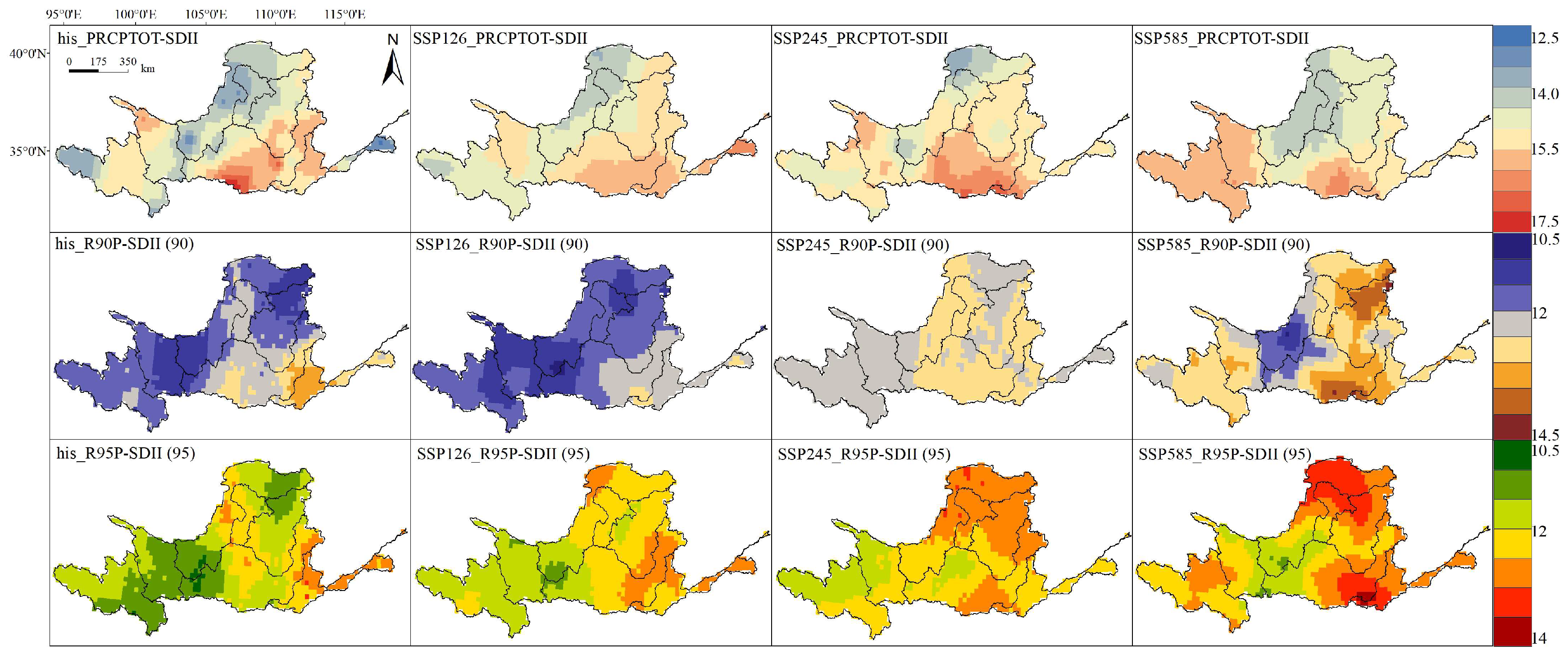
Using the Kendall rank correlation coefficient to test the correlations between three indices (PRCPTOT-SDII, R90P-SDII (90), and R90P-SDII (95)) (Figure 2), the results indicate that as precipitation became more extreme, the correlation between precipitation amount and precipitation intensity weakened, specifically Corr (PRCPTOT-SDII) > Corr (R90P-SDII (90)) > Corr (R95P-SDII (95)). With an increase in radiative intensity, the correlation between the precipitation amount and precipitation intensity became stronger, with CorrSSP126 (PRCPTOT-SDII) > CorrSSP245 (PRCPTOT-SDII) > CorrSSP585 (PRCPTOT-SDII). Spatially, there was noticeable spatial continuity in the correlation between the precipitation amount and precipitation intensity, mirroring the spatial distribution of the precipitation amount by generally exhibiting a southeast-to-northwest decreasing trend. In regions with high precipitation amounts, the correlation between precipitation amount and precipitation intensity was stronger.
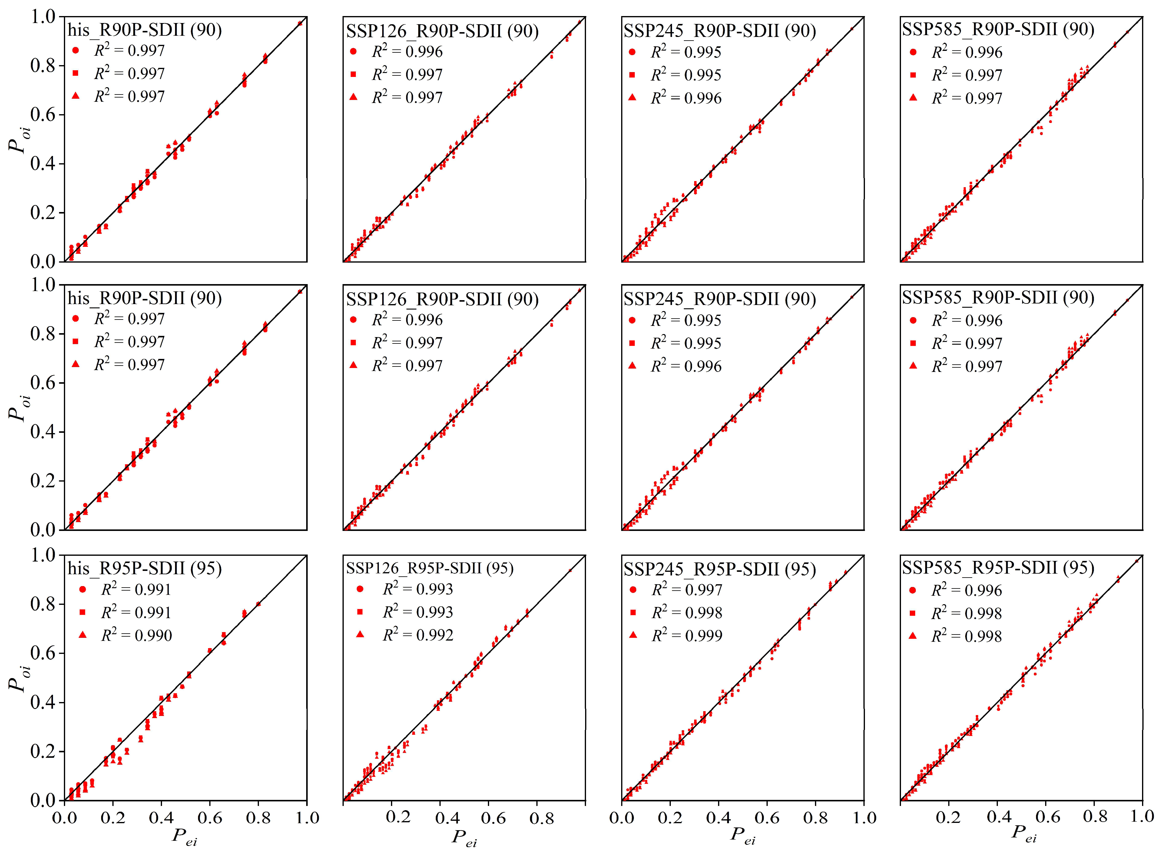
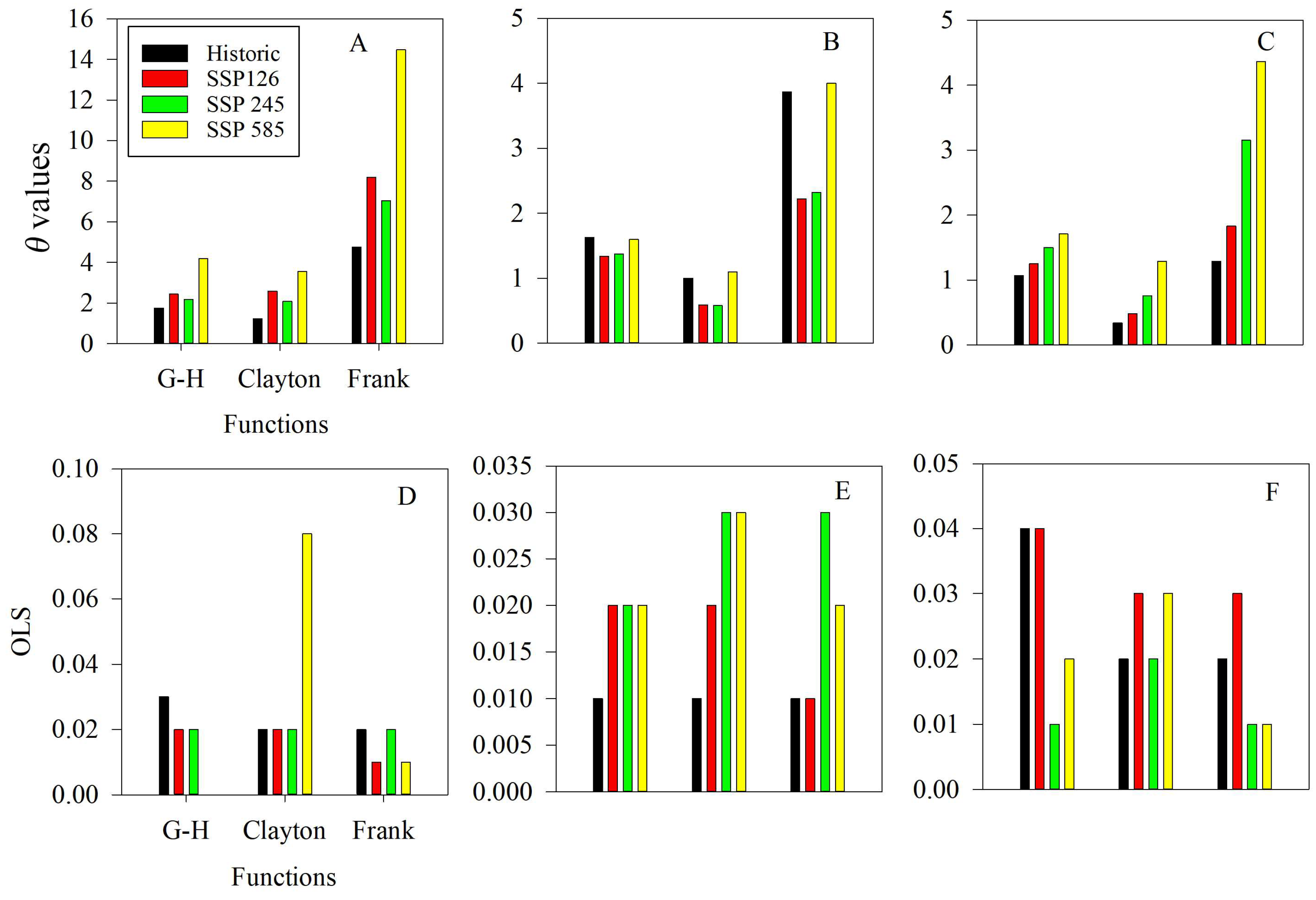
Based on the graphical analysis and taking the upstream “Jiuzhi” station in the watershed as an example (Figure 3), in the context of the two-dimensional empirical points and theoretical data points, there was a relatively uniform distribution on both sides of the 45-degree line. The differences between the three Archimedean copulas were not significant, and all of them could effectively describe the dependence between the indices. The coefficients of determination (R2) for the functional fits were all greater than 0.99. The fit of the empirical points for the three two-dimensional joint distributions was similar. The Gumbel copula and Frank copula tended to underestimate the observed points, while the Clayton copula tended to overestimate the observed points (Figure 3). Combining the graphical analysis with the Ordinary Least Squares (OLS) minimum criterion (Figure 4), the results indicate that during the historical period, the Clayton copula provided the best description for the PRCPTOT-SDII index, the Frank copula was optimal for the R90P-SDII (90) index, and the Clayton copula was optimal for the R95P-SDII (95) index. Similarly, the optimal copula functions could be obtained for various indices between other stations within the watershed, both historical and future.
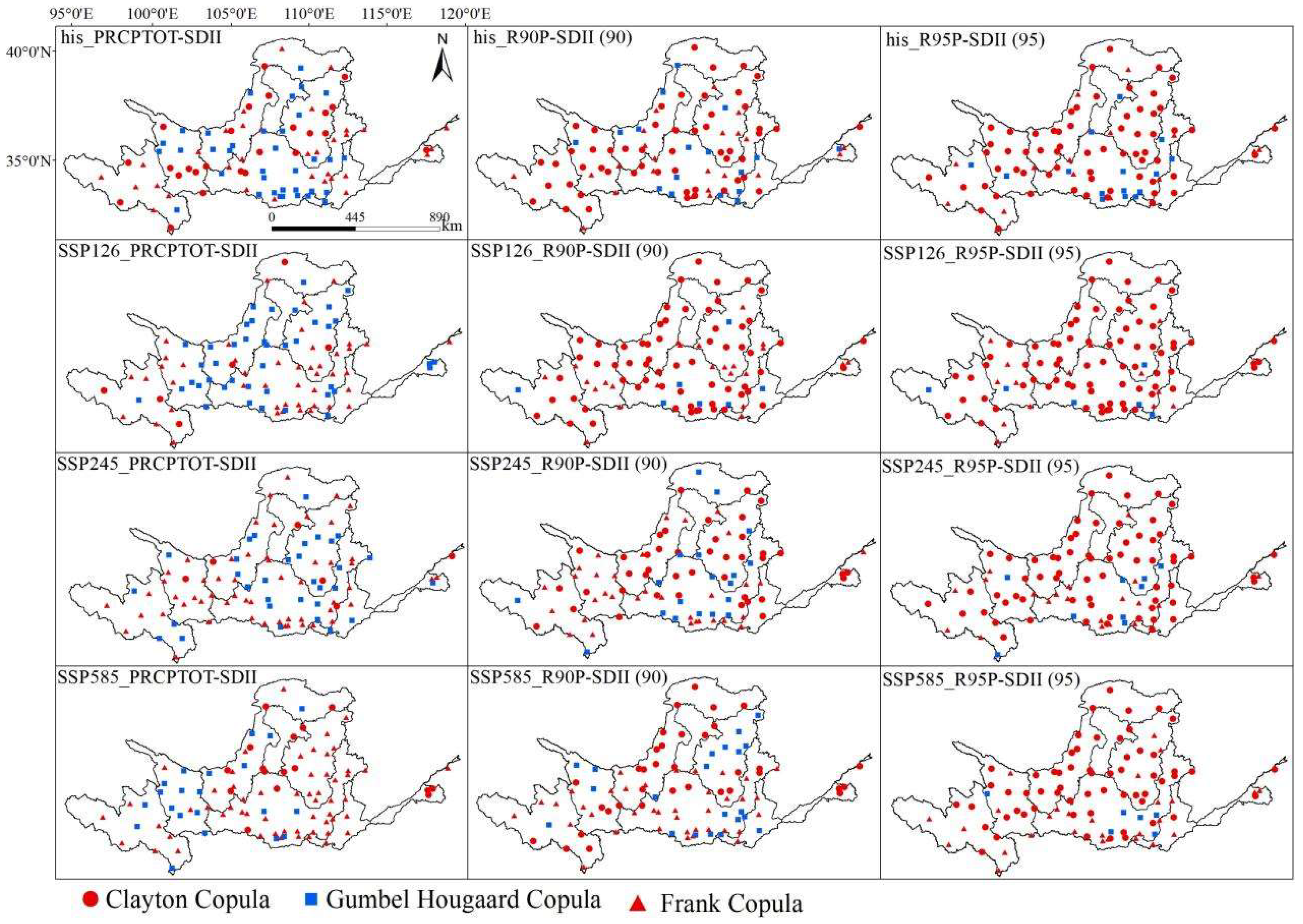
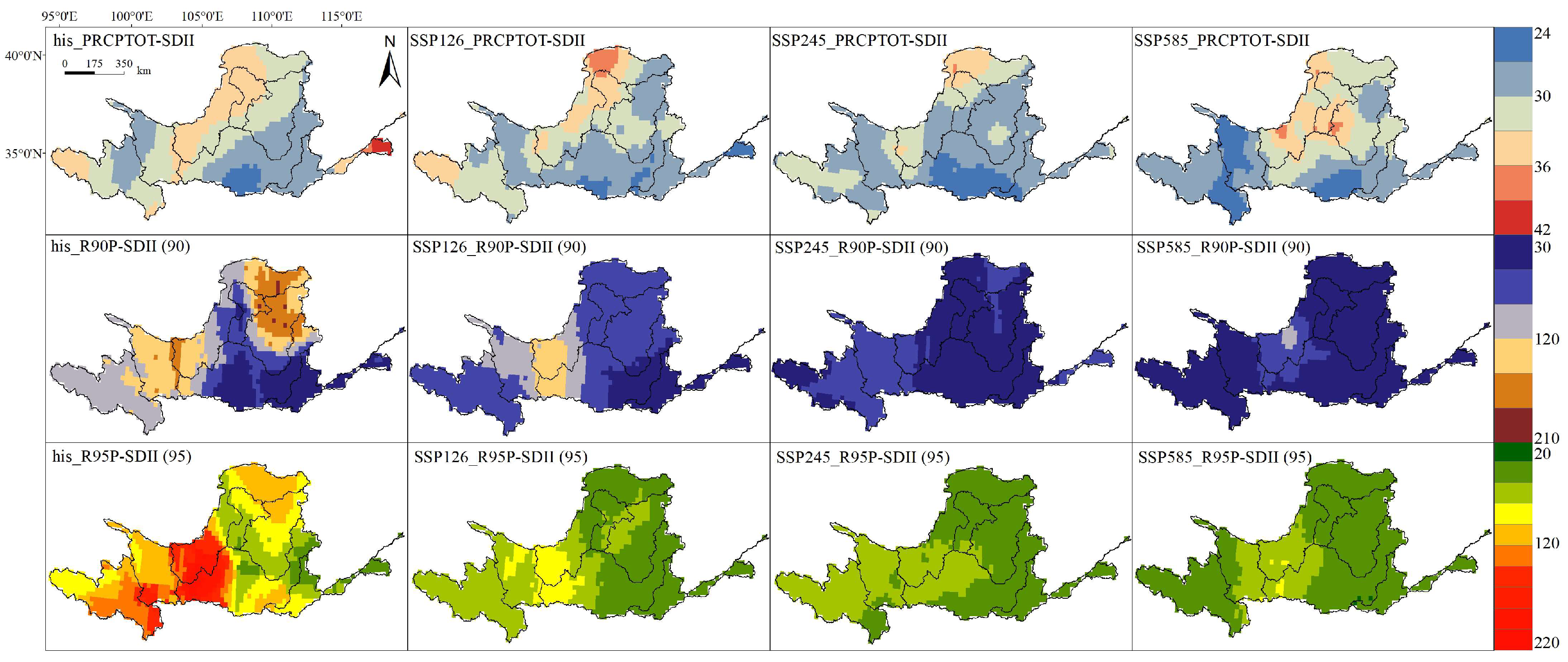
There was a clear spatial pattern in the optimal copula functions among the indices within the watershed (Figure 5). Overall, when the G-H copula function was considered as the optimal copula function, it tended to be more distributed in the midstream of the watershed. When the Frank copula function was the optimal choice, it was more prevalent in the upstream and downstream regions of the watershed. Looking specifically at the index pairs (Figure 6), the Frank copula function provided the best description of the dependence between the PRCPTOT-SDII index pairs, with proportions of 35.1%, 48.9%, 59.6%, and 60.6% for the historical and SSP126, SSP245, and SSP585 scenarios, respectively. The Clayton copula function was optimal for describing the dependence between the R90P-SDII (90) index pairs, with proportions of 56.4%, 67.0%, 44.7%, and 37.2% for the historical and SSP126, SSP245, and SSP585 scenarios, respectively. The Clayton copula was also the optimal choice for describing the dependence between the R95P-SDII (95) index pairs, with proportions of 68.1%, 78.7%, 69.1%, and 63.8% for the historical and SSP126, SSP245, and SSP585 scenarios, respectively. In general, the Clayton copula was selected more frequently as the optimal copula function as quantile values increased. This suggests that the Clayton copula has an advantage over the other two Archimedean copulas in describing the joint probability distribution of extreme events.

3.2. Bivariate Recurrence Period

The index combining the precipitation amount and precipitation intensity represents the magnitude and intensity of precipitation occurring simultaneously in the region throughout the year. If the probability of both occurring together is high or the design value is significant, it indicates that the region is prone to exposure to extreme precipitation with high amounts and intensity. This categorizes it as an area susceptible to extreme precipitation with a higher likelihood of experiencing flooding disasters. Using the selected copula functions in Equations (3)–(5). We calculated the joint recurrence periods, coincident recurrence periods, and Kendall recurrence periods between the three index pairs (PRCPTOT-SDII, R90P-SDII (90), and R95P-SDII (95)) under different scenarios for historical and future periods and the given single-variable recurrence periods (2a, 5a, 10a, 20a, 50a, and 100a). This analysis aided in identifying regions within the watershed that are prone to extreme precipitation.
As the single-variable recurrence periods increased, the joint recurrence period, coincident recurrence period, and Kendall recurrence period all increased. This suggests an inseparable inherent relationship between extreme precipitation indices, with larger single-variable recurrence periods corresponding to greater increases in these three recurrence periods. Bivariate recurrence periods exhibit significant spatial differences. Taking the example of the R90P-SDII (90) index under a 20-year recurrence period, the difference between the maximum and minimum joint recurrence periods within the Yellow River Basin is 1.4 times, that of the coincident recurrence period is 7.0 times, and that of the Kendall recurrence period is 4 times, and this difference increases with larger recurrence periods. Similar bivariate recurrence periods under the same recurrence period show distinct differences among the index pairs, with the pattern being PRCPTOT-SDII < R90P-SDII (90) < R95P-SDII (95). For instance, in terms of the Kendall recurrence period, the maximum value of PRCPTOT-SDII is 1.8 times the minimum value, that of R90P-SDII (90) is 4.0 times, and that of R95P-SDII (95) is 4.0 times.
Using a 20-year single-variable recurrence period as an example, the spatial distribution characteristics of bivariate recurrence periods are shown in Figure 7, Figure 8 and Figure 9. For the joint recurrence period (Figure 7), its distribution was similar to that of the corresponding extreme precipitation indices, generally decreasing from southeast to northwest and with a larger variability in recurrence rates from southeast to northwest. The smaller joint recurrence periods indicated a higher likelihood of large precipitation amounts or intense precipitation occurring separately during the year, implying a lower risk of concentrated extreme precipitation in these areas. High-value areas were located in the southern and northwestern parts of the basin, including the Weihe River, Yiluo River, and parts of the Jinghe River Basin. Low-value areas were found in the middle reaches of the basin, from Lanzhou to Huayuankou, including the Kuye River Basin. Compared to the historical periods, the joint recurrence periods tended to decrease in future scenarios, possibly due to different sequence lengths. For the coincident recurrence periods and Kendall recurrence periods (Figure 8 and Figure 9), their distributions were opposite to those of the corresponding extreme precipitation indices, showing an overall increasing trend from southeast to northwest. Lower joint recurrence periods indicated a higher probability of encountering heavy rainfall and intense precipitation events, implying a greater flood risk in these areas. Figure 9 and Figure 10 demonstrate that low-value areas were located in the southeastern part of the basin, where precipitation was abundant and concentrated, resulting in a higher probability of extreme precipitation risk. High-value areas were situated in the northwestern part of the basin, mainly from Lanzhou to Huayuankou, where precipitation was abundant but less intense, indicating a higher number of rainy days and dispersed precipitation, resulting in a lower risk of extreme precipitation.
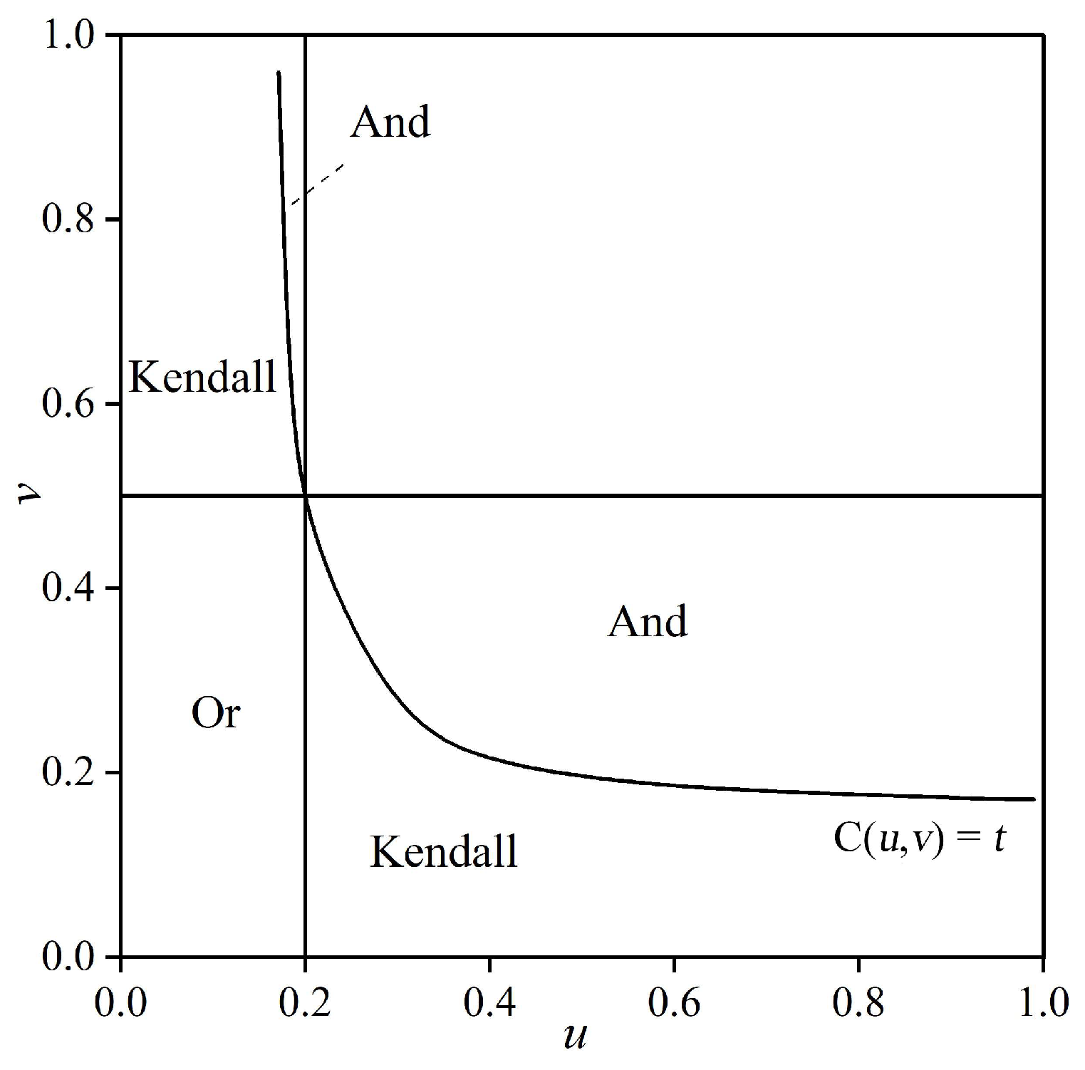
The probability order of the four recurrence periods is as follows: TAnd > TKendall > TSingle-variable > TOr. The joint recurrence period (Or) and coincident recurrence period (And) can be considered as the maximum and minimum extremes under single-variable recurrence periods, serving as the estimated range for actual recurrence periods. The patterns during recurrence periods can be explained from the perspective of safety thresholds and danger thresholds. Figure 10 describes the safety threshold ranges identified by three recurrence periods (the Kendall recurrence period, coincident recurrence period, and joint recurrence period). The safety threshold range identified by the joint recurrence period (Or) is the rectangular area in the lower left corner, while the Kendall recurrence period defines the lower part of the curve C(u,v) as the safety zone. The coincident recurrence period, building upon the Kendall recurrence period, further adds the And part as a safety threshold region. It can be observed that the danger threshold range defined by the Kendall recurrence period is not excessively large or small compared to the coincident recurrence period and joint recurrence period. This ensures engineering safety while avoiding excessive costs. Thus, this paper used the Kendall recurrence period as the recurrence period design for two-dimensional joint distribution.

3.3. Bivariate Design Values

As shown in the contour plots (Figure 11), several combinations of extreme precipitation characteristics satisfied a certain joint probability under a given recurrence period. In this study, the maximum likelihood method was used to find the combination design values that maximized the probability of occurrence under the specified Kendall recurrence periods (2a, 5a, 10a, 20a, 50a, and 100a). Larger combination design values under a given Kendall recurrence period indicated a higher probability of extreme precipitation in that region. According to Table 5, under the influence of climate change, the future bivariate design values showed variations ranging from 6.76% to 28.8% compared to historical periods. The increase in magnitude was observed to be greater with increasing radiative forcing scenarios, with a trend of SSP126 < SSP245 < SSP585. The bivariate design values were significantly different from the single-variable design values, with variations ranging from −0.79% to −18.67%. This difference increased with higher quantiles, as shown by R95P-SDII (95) > R90P-SDII (90) > PRCPTOT-SDII.
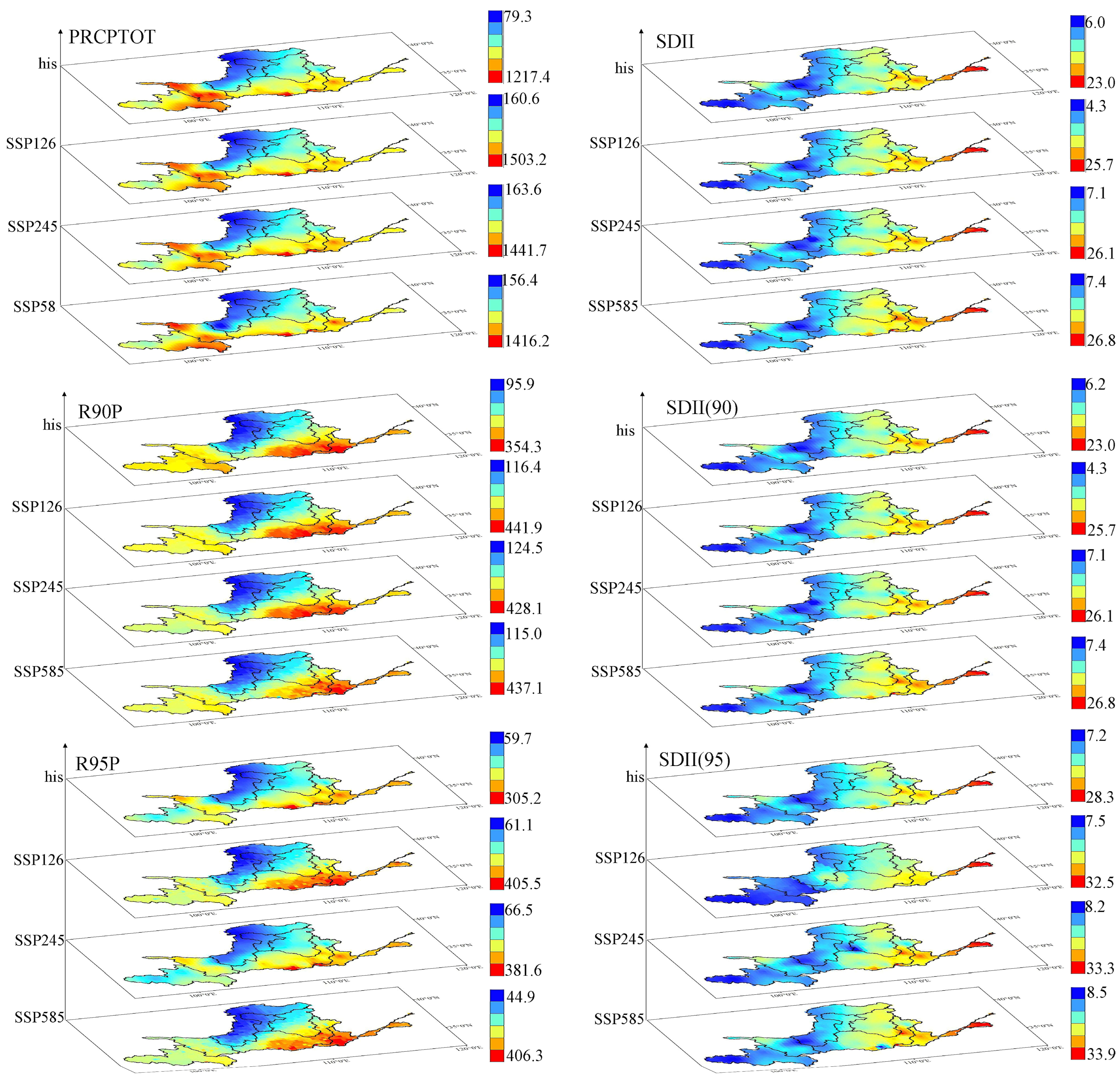
The bivariate design values for different return periods under historical and future scenarios are shown in Figure 12. The spatial patterns of the bivariate design values of the three index pairs showed relatively small changes between the historical and future scenarios and were generally consistent with the spatial patterns of their respective extreme precipitation indices. Overall, they showed an eastern surplus and a western deficit, with more in the south and less in the north. For PRCPTOT-SDII, the downstream areas of the basin were characterized as high-value regions, while the northern part of the middle reaches was a low-value region, with noticeable differences between high- and low-value areas. Differences in the SDII and PRCPTOT design value spatial patterns were mainly concentrated in the middle and upper reaches of the basin, where precipitation was abundant but less intense, indicating a significantly higher number of rainy days compared to other regions. For the R90P-SDII (90) index pair, differences compared to the PRCPTOT-SDII index pair were mainly observed in the upstream region of the basin. This shows that the proportion of extreme precipitation was significantly lower in the upstream region, meaning that extreme precipitation occurred less frequently in the upstream region, while the southeastern part of the basin showed the opposite trend. The spatial pattern of the SDII (90) index confirmed that the downstream region of the basin experienced higher intensity of extreme precipitation, and the probability of short duration heavy rainfall events was greater compared to the upstream region. For the R95P-SDII (95) index pair, the spatial patterns of the bivariate design values under historical and future scenarios were similar to those of R90P-SDII (90). The main difference was the greater contrast between high- and low-value areas, which increased with increased radiative forcing.

4. Discussion

While there has been increasing attention paid to the prediction of precipitation runoff under the influence of climate change [32,33], relatively little research has focused specifically on the contribution of extreme precipitation to runoff. This study investigated extreme precipitation and its differences from regular precipitation by analyzing the extreme annual precipitation and corresponding extreme precipitation intensity indices at different quantiles. The results show that the correlation between the annual precipitation and precipitation intensity decreased with increasing quantiles, and the relationship is shown as PRCPTOT-SDII > R90P-SDII (90) > R95P-SDII (95). The correlation between precipitation amount and intensity was weaker and in some cases negative for extreme precipitation conditions. This may be related to the different contributions of weather systems to precipitation of different intensities [34,35], making the relationship between precipitation characteristics more complex for extreme precipitation. Extreme precipitation has a higher degree of randomness compared to normal precipitation [36]. To place these findings in context, it is important to compare them with previous research in this area. Previous studies have also examined the relationship between extreme precipitation and runoff in various regions [37,38]. However, our research uniquely focused on the Yellow River Basin, where extreme precipitation events have significant implications for flood risk. Our results corroborate earlier findings regarding the increasing complexity of the relationship between precipitation amount and intensity, particularly in the context of extreme precipitation.
To estimate the tail distribution of correlated environmental variables (e.g., precipitation and wind speed) and to account for interdependencies between variables, copula functions have become the standard tool for describing joint distributions of hydrological variables. However, the optimal type of copula function for describing the dependence between hydrological extremes remains unclear among numerous choices. This study shows that three commonly used Archimedean copula functions exhibited regular patterns for the three index pairs in both spatial and index-related contexts. With increasing quantiles, the correlation between precipitation amount and precipitation intensity weakened, and the optimal copula function gradually shifted from the Frank copula to the Clayton copula. This was due to the properties of the copula functions and their relationship with the indices. The Frank copula was better at capturing upper-tail correlations, while the Clayton copula was better at modeling lower-tail, heavy-tailed relationships [39,40,41]. This advantage was consistent across historical and future scenarios, suggesting that climate change has a relatively small impact on the dependence between extreme precipitation indices. Therefore, the Clayton copula is recommended as a preferred alternative for modeling multivariate dependence in extreme precipitation studies compared to other copula functions.
In comparison to previous research on copula functions, our study provides insights into the suitability of specific copula functions for modeling the dependence between extreme precipitation indices. Our findings reinforce the utility of the Clayton copula in capturing lower-tail relationships, particularly in the context of extreme precipitation. This has significant implications for the accurate modeling of multivariate dependence in extreme precipitation studies.
Based on the bivariate recurrence periods and design values, this study identified regions prone to extreme precipitation events of high magnitude and intensity occurring simultaneously. When increasing the given return periods (2a, 5a, 10a, 20a, 50a, and 100a), all three bivariate return periods increased, indicating an inherent, inseparable relationship between the extreme precipitation indices. Moreover, as the given recurrence period increased, the variations in these three recurrence periods became larger. The observed pattern was that the coincident recurrence period increased the most, followed by the Kendall recurrence period and then the joint recurrence period. For a 100a recurrence period, the difference between the single-variable recurrence periods and the coincident recurrence periods could be several hundred times larger. This phenomenon may be related to the properties of copula functions, as the estimation error of out-of-sample frequency values increases with higher frequencies. Therefore, when using copula functions in multivariate analysis, estimates for smaller return periods are more reliable and appropriate [42,43].
In terms of hydrological frequency analysis, our research contributes to a deeper understanding of the impact of different return periods on bivariate recurrence periods. Our findings emphasize the importance of considering the reliability and appropriateness of estimates for smaller return periods in multivariate analysis, which can significantly affect the assessment of flood risk.
Due to the inconsistency in the time series length between the historical and future periods in this study, the bivariate return periods showed greater spatial differences in historical periods compared to future scenarios. Therefore, the length and consistency of time series are important considerations in studies investigating hydrological frequency analysis under climate change. Longer and more consistent time series can capture more characteristics, improve representativeness, and enhance comparability, leading to more reliable results in hydrological forecasting [44,45].
In comparing historical and future scenarios, our research underscores the significance of the time series length and consistency in the context of hydrological frequency analysis. The differences observed between historical and future periods are a critical consideration for researchers and policymakers when assessing the potential impact of climate change on extreme precipitation events.
Lower joint return periods indicate a higher likelihood of large amounts of precipitation or intense precipitation occurring separately during the year. This implies a greater likelihood of heavy precipitation events with large precipitation amounts and intensities, which means a higher risk of flooding in these areas. Overall, the southern part of the middle and upper reaches and the downstream areas of the basin are prone to extreme precipitation, while the northern part of the middle reaches is less prone [46,47,48]. Compared to historical periods, the common return periods tend to decrease in future scenarios, possibly due to different time series lengths. Similarly, regions with larger design values for given Kendall recurrence intervals have a higher probability of experiencing extreme precipitation events. The identified regions prone to extreme precipitation based on bivariate design values for PRCPTOT-SDII, R90P-SDII (90), and R95P-SDII (95) were consistent with the recurrence period-based identifications. The contrasting index pairs at different quantiles show that as precipitation becomes more extreme, high-precipitation areas shift from the southern upstream and southeastern parts of the basin to the more southeastern parts, indicating a greater likelihood of concentrated heavy rainfall in downstream areas compared to other basin regions, making them flood-prone areas. This could be due to the southeastern region of the basin being influenced by the monsoon, which is more sensitive to temperature increases [49,50]. In the same region, future bivariate design values are larger than those in historical periods, indicating a significant increase in extreme precipitation risk within the basin under the influence of climate change. In addition, the differences between the high and low values became more pronounced with increasing radiative forcing, suggesting that climate change may exacerbate the differences between wet and dry regions [4].
In the context of regional flood risk assessment, our research provides valuable insights into the geographic areas prone to extreme precipitation events and the potential changes in these patterns under the influence of climate change. These findings have implications for disaster management and planning in the Yellow River Basin and similar regions.

5. Conclusions

This study focused on the analysis of extreme annual precipitation and the associated extreme precipitation intensity indices at different quantiles in the Yellow River Basin. Copula functions were employed to assess the bivariate return periods and design values of the extreme precipitation indices for both historical and future scenarios, allowing us to identify regions within the Yellow River Basin that are prone to extreme precipitation events. Our analysis demonstrated that three Archimedean copula functions are well suited for modeling the joint distribution of precipitation amount and intensity indices at different quantiles in the Yellow River Basin. Among these, the Clayton copula exhibited a significant advantage, particularly as precipitation became more extreme. Therefore, the Clayton copula stands out as a preferable choice for the multivariate modeling of extreme precipitation events in this region. In summary, our findings identified the upper reaches in the southern and downstream regions of the basin as areas susceptible to extreme precipitation, including the Weihe River, Yellow River, and parts of the Jing River Basin. In contrast, the northern middle reaches from Lanzhou to Huayuankou were characterized as low-susceptibility areas, including the Kuye River Basin. As precipitation becomes more extreme, the high-precipitation area in the upper reaches gradually decreases, and the high-precipitation area in the southeastern downstream region also shifts to the southern downstream region. This shift suggests a higher probability of concentrated heavy precipitation events in the downstream area compared to other parts of the basin, especially under high radiative forcing scenarios.
As we conclude this study, it is important to consider future research directions in the field of extreme precipitation and hydrological risk assessment. Subsequent studies may benefit from further investigation of the impact of climate change on extreme precipitation in the Yellow River Basin, with a focus on specific climate model projections and scenarios. Additionally, the application of advanced statistical and hydrological models can enhance the accuracy of flood risk assessments. The proposed model based on copula functions was proven to be effective in characterizing the joint distribution of extreme precipitation indices. It provides valuable insights into the spatial and temporal patterns of extreme precipitation in the Yellow River Basin. However, it is important to acknowledge certain limitations of the model, including the assumptions and simplifications inherent in copula functions. Further research is needed to explore alternative modeling approaches that can address these limitations and improve the precision of extreme precipitation risk assessments.

Author Contributions

Conceptualization, G.Z.; methodology, F.L.; software, F.L.; validation, G.Z.; formal analysis, G.Z.; investigation, F.L.; resources, F.L.; data curation, G.Z.; writing—original draft preparation, G.Z.; writing—review and editing, F.L.; supervision, X.Z.; project administration, G.Z.; funding acquisition, X.Z. All authors have read and agreed to the published version of the manuscript.

Funding

This project was funded by the Huang Committee Outstanding Young Talents Science and Technology Project (HQK-202305) (Guodong, Zhang) and Qian Kehe Zhicheng (2023) Yiban 206 (Xueli, Zhang).

Data Availability Statement

Data sharing is not applicable to this article.

Conflicts of Interest

The authors declare no conflict of interest.

References

  1. Wang, S.; Fu, B.; Piao, S. Reduced sediment transport in the Yellow River due to anthropogenic changes. Nat. Geosci. 2016, 9, 38–41. [Google Scholar] [CrossRef]
  2. Chen, Y.; Fu, B.; Zhao, Y.; Wang, K.; Zhao, M.; Ma, J.; Wu, J.; Xu, C.; Liu, W.; Wang, H. Sustainable development in the Yellow River Basin: Issues and strategies. J. Clean. Prod. 2020, 263, 121223. [Google Scholar] [CrossRef]
  3. Zhao, Y.; Xu, X.; Huang, W.; Wang, Y.; Xu, Y.; Chen, H.; Kang, Z. Trends in observed mean and extreme precipitation within the Yellow River Basin, China. Theor. Appl. Climatol. 2019, 136, 1387–1396. [Google Scholar] [CrossRef]
  4. Gao, T.; Wang, H. Trends in precipitation extremes over the Yellow River basin in North China: Changing properties and causes. Hydrol. Process. 2017, 31, 2412–2428. [Google Scholar] [CrossRef]
  5. Jiang, S.; Cui, H.; Ren, L.; Yan, D.; Yang, X.; Yuan, S.; Liu, Y.; Wang, M.; Xu, C. Will China’s Yellow River basin Suffer More Serious Combined Dry and Wet Abrupt Alternation in the Future? J. Hydrol. 2023, 624, 129871. [Google Scholar] [CrossRef]
  6. Zhang, Y.; Liang, K.; Liu, C. Time distribution pattern and spatial heterogeneity of hourly scale event-based extreme precipitation in China. J. Hydrol. 2023, 622, 129712. [Google Scholar] [CrossRef]
  7. Donat, M.G.; Delgado-Torres, C.; De Luca, P.; Mahmood, R.; Ortega, P.; Doblas-Reyes, F.J. How credibly do CMIP6 simulations capture historical mean and extreme precipitation changes? Geophys. Res. Lett. 2023, 50, e2022GL102466. [Google Scholar] [CrossRef]
  8. Deng, R.; Qiao, S.; Zhu, X.; Dong, T.; Feng, G.; Dong, W. The improvements of sea surface temperature simulation over China Offshore Sea in present climate from CMIP5 to CMIP6 models. Clim. Dyn. 2023, 61, 5111–5130. [Google Scholar] [CrossRef]
  9. Nooni, I.K.; Ogou, F.K.; Chaibou, A.A.S.; Natoky, F.M.; Gnitou, G.T.; Lu, J. Evaluating CMIP6 Historical Mean Precipitation over Africa and the Arabian Peninsula against Satellite-Based Observation. Atmosphere 2023, 14, 607. [Google Scholar] [CrossRef]
  10. Yu, X.; Zhang, L.; Zhou, T.; Zheng, J. Assessing the performance of CMIP6 models in simulating droughts across global drylands. Adv. Atmos. Sci. 2023, 1–16. [Google Scholar] [CrossRef]
  11. Janizadeh, S.; Bateni, S.M.; Jun, C.; Pal, S.C.; Band, S.S.; Chowdhuri, I.; Saha, A.; Tiefenbacher, J.; Mosavi, A. Potential impacts of future climate on the spatio-temporal variability of landslide susceptibility in Iran using machine learning algorithms and CMIP6 climate-change scenarios. Gondwana Res. 2023, 124, 1–17. [Google Scholar] [CrossRef]
  12. Reddy, N.M.; Saravanan, S. Extreme precipitation indices over India using CMIP6: A special emphasis on the SSP585 scenario. Environ. Sci. Pollut. Res. 2023, 30, 47119–47143. [Google Scholar] [CrossRef] [PubMed]
  13. Mmame, B.; Ngongondo, C. Evaluation of CMIP6 model skills in simulating tropical climate extremes over Malawi, Southern Africa. Model. Earth. Syst. Environ. 2023, 1–15. [Google Scholar] [CrossRef]
  14. Ding, Y.; Jiang, C.; Zhou, Z.; Gao, T.; Wang, S.; Zhang, X.; Cai, H.; Shi, H. Evaluation of precipitation and its time series components in CMIP6 over the Yellow River Basin. Clim. Dyn. 2023, 60, 1203–1223. [Google Scholar] [CrossRef]
  15. Chen, T.; Ao, T.; Zhang, X.; Li, X.; Zhou, L.; Li, M.; Yang, K. Spatial and temporal variation and probability characteristics of extreme precipitation events in the Min River Basin from 1961 to 2016. Appl. Ecol. Environ. Res. 2019, 17, 11375–11394. [Google Scholar] [CrossRef]
  16. Innocenti, S.; Mailhot, A.; Leduc, M.; Cannon, A.J.; Frigon, A. Projected changes in the probability distributions, seasonality, and spatiotemporal scaling of daily and subdaily extreme precipitation simulated by a 50-member ensemble over northeastern North America. J. Geophys. Res. Atmos. 2019, 124, 10427–10449. [Google Scholar] [CrossRef]
  17. Murphy, C.; Kettle, A.; Meresa, H.; Golian, S.; Bruen, M.; Mellander, P.; Tsakiris, G. Climate Change Impacts on Irish River Flows: High Resolution Scenarios and Comparison with CORDEX and CMIP6 Ensembles. Water Resour. Manag. 2023, 37, 1841–1858. [Google Scholar] [CrossRef]
  18. Das, P.; Zhang, Z.; Ghosh, S.; Lu, J.; Ayugi, B.; Ojara, M.; Guo, X. Historical and projected changes in Extreme High Temperature events over East Africa and associated with meteorological conditions using CMIP6 models. Glob. Planet Chang. 2023, 222, 104068. [Google Scholar] [CrossRef]
  19. Konda, G.; Vissa, N.K. Evaluation of CMIP6 models for simulations of surplus/deficit summer monsoon conditions over India. Clim. Dyn. 2023, 60, 1023–1042. [Google Scholar] [CrossRef]
  20. Taylor, G.P.; Loikith, P.C.; Aragon, C.M.; Lee, H.; Waliser, D.E. CMIP6 model fidelity at simulating large-scale atmospheric circulation patterns and associated temperature and precipitation over the Pacific Northwest. Clim. Dyn. 2023, 60, 2199–2218. [Google Scholar] [CrossRef]
  21. Pierce, D.W.; Cayan, D.R.; Feldman, D.R.; Risser, M.D. Future Increases in North American Extreme Precipitation in CMIP6 Downscaled with LOCA. J. Hydrometeorol. 2023, 24, 951–975. [Google Scholar] [CrossRef]
  22. Sarkar, S.; Maity, S.S.; Maity, R. Precipitation-based Climate Change Hotspots across India through a Multi-model Assessment from CMIP6. J. Hydrol. 2023, 623, 129805. [Google Scholar] [CrossRef]
  23. Wang, S.; Feng, J.; Liu, X.; Ji, X. Simulation of the long-term variability of the Hadley circulation in CMIP6 models. Atmos. Res. 2023, 287, 106716. [Google Scholar] [CrossRef]
  24. Gadain, H.; Libanda, B. CMIP6 models simulate heavier future rainfall over the Highlands than across other agricultural areas of Yemen. Model. Earth. Syst. Environ. 2023, 1–13. [Google Scholar] [CrossRef]
  25. Zhang, Y.; Chiew, F.H.S.; Li, M.; Post, D. Predicting Runoff Signatures Using Regression and Hydrological Modeling Approaches. Water Resour. Res. 2018, 54, 125478. [Google Scholar] [CrossRef]
  26. Galelli, S.; Castelletti, A. Assessing the predictive capability of randomized tree-based ensembles in streamflow modelling. Hydrol. Earth. Syst. Sci. 2013, 17, 2669–2684. [Google Scholar] [CrossRef]
  27. Sklar, A. Fonctions de Repartition an Dimensions et Leurs Marges. Publ. Inst. Statist. Univ. Paris 1959, 8, 229–231. [Google Scholar]
  28. Bajracharya, A.R.; Bajracharya, S.R.; Shrestha, A.B.; Maharjan, S.B. Climate change impact assessment on the hydrological regime of the Kaligandaki Basin, Nepal. Sci. Total Environ. 2018, 625, 837–848. [Google Scholar] [CrossRef]
  29. Shrestha, N.K.; Du, X.; Wang, J. Assessing climate change impacts on fresh water resources of the Athabasca River basin, Canada. Sci. Total Environ. 2017, 601, 425–440. [Google Scholar] [CrossRef]
  30. Nejc, B.; Mojca, Š.; Matjaž, M. Copula-based IDF curves and empirical rainfall thresholds for flash floods and rainfall-induced landslides. J. Hydrol. 2016, 541, 272–284. [Google Scholar] [CrossRef]
  31. Salvatore, G.; Francesco, S. Asymmetric copula in multivariate flood frequency analysis. Adv. Water Resour. 2006, 29, 1155–1167. [Google Scholar] [CrossRef]
  32. Halwatura, D.; Najim, M.M.M. Application of the HEC-HMS model for runoff simulation in a tropical catchment. Environ. Model. Softw. 2013, 46, 155–162. [Google Scholar] [CrossRef]
  33. Muhammad, A.; Minha, C.; Tae-Woong, K.; Umar, W.L. Hydrological modeling to simulate streamflow under changing climate in a scarcely gauged cryosphere catchment. Environ. Earth Sci. 2016, 75, 186. [Google Scholar] [CrossRef]
  34. Yuan, W.L.; Liu, M.Q.; Wang, F. Calculation of Critical Rainfall for Small-Watershed Flash Floods Based on the HEC-HMS Hydrological Model. Water Resour. Manag. 2019, 33, 2555–2575. [Google Scholar] [CrossRef]
  35. Ran, G.; Jian, S.; Wu, Q.; Zhang, L.; Hu, C. Exploring the Dominant Runoff Processes in Two Typical Basins of the Yellow River, China. Water 2020, 12, 3055. [Google Scholar] [CrossRef]
  36. Luo, L.; Wang, Z.J.; Liu, X.Y.; Zhang, X.C. Changes in characteristics of precipitation in flood season over five typical basins of middle reaches of the yellow River in China. J. Hydraul. Eng. 2013, 44, 848–855, (In Chinese with English abstract). [Google Scholar]
  37. Ren, Z.; Ma, X.; Wang, K.; Li, Z. Effects of Extreme Precipitation on Runoff and Sediment Yield in the Middle Reaches of the Yellow River. Atmosphere 2023, 14, 1415. [Google Scholar] [CrossRef]
  38. Chang, D.; Li, S.; Lai, Z. Effects of extreme precipitation intensity and duration on the runoff and nutrient yields. J. Hydrol. 2023, 626, 130281. [Google Scholar] [CrossRef]
  39. Mohammad, R.R.; Fernanda, H.; Bofu, Y. Individual and combined impacts of urbanization and climate change on catchment runoff in Southeast Queensland, Australia. Sci. Total Environ. 2023, 861, 160528. [Google Scholar] [CrossRef]
  40. José, Y.G.; Suzana, M.G.; Richarde, M.; Celso, A.G. Modeling the impacts of future LULC and climate change on runoff and sediment yield in a strategic basin in the Caatinga/Atlantic forest ecotone of Brazil. Catena 2021, 203, 105308. [Google Scholar] [CrossRef]
  41. Utsumi, N.; Kim, H.; Kanae, S.; Oki, T. Relative contributions of weather systems to mean and extreme global precipitation. J. Geophys. Res. Atmos. 2016, 122, 152–167. [Google Scholar] [CrossRef]
  42. Li, J.; Qian, Y.; Leung, L.R.; Feng, Z. Summer mean and extreme precipitation over the Mid-Atlantic Region: Climatological characteristics and contributions from different precipitation types. J. Geophys. Res. Atmos. 2021, 126, e2021JD035045. [Google Scholar] [CrossRef]
  43. Gimeno, L.; Sorí, R.; Vázquez, M.; Stojanovic, M.; Algarra, I.; Eiras-Barca, J.; Gimeno-Sotelo, L.; Nieto, R. Extreme precipitation events. WIREs Water 2022, 9, e1611. [Google Scholar] [CrossRef]
  44. Naz, S.; Jamil, S.S.; Iqbal, M.J. Archimedean copula-based bivariate flood-frequency analysis on Sukkur, Pakistan. Arab J. Geosci. 2020, 13, 282. [Google Scholar] [CrossRef]
  45. Wable, P.S.; Jha, M.K. Application of Archimedean copulas to the impact assessment of hydro-climatic variables in semi-arid aquifers of western India. Hydrogeol. J. 2018, 26, 89–108. [Google Scholar] [CrossRef]
  46. Wazneh, H.; Arain, M.A.; Coulibaly, P.; Gachon, P.T.; Rigo, T. Evaluating the dependence between temperature and precipitation to better estimate the risks of concurrent extreme weather events. Adv. Meteorol. 2020, 2020, 8763631. [Google Scholar] [CrossRef]
  47. Brunner, M.I.; Liechti, K.; Zappa, M. Extremeness of recent drought events in Switzerland: Dependence on variable and return period choice. Nat. Hazards Earth Syst. Sci. 2019, 19, 2311–2323. [Google Scholar] [CrossRef]
  48. Bender, J.; Wahl, T.; Jensen, J. Multivariate design in the presence of non-stationarity. J. Hydrol. 2014, 514, 123–130. [Google Scholar] [CrossRef]
  49. Jiang, C.; Xiong, L.; Yan, L.; Dong, J.; Xu, C. Multivariate hydrologic design methods under nonstationary conditions and application to engineering practice. Hydrol. Earth Syst. Sci. 2019, 23, 1683–1704. [Google Scholar] [CrossRef]
  50. Zhu, X.; Lee, S.Y.; Wen, X.; Ji, Z.; Lin, L.; Zheng, Z.; Xu, D.; Dong, W. Extreme climate changes over three major river basins in China as seen in CMIP5 and CMIP6. Clim. Dyn. 2021, 57, 1187–1205. [Google Scholar] [CrossRef]
Figure 1. Study area.
Water 15 03957 g001
Figure 2. Correlation between extreme precipitation index pairs.
Water 15 03957 g002
Figure 3. Cooperation between the two-dimensional empirical estimates and theoretical estimates.
Water 15 03957 g003
Figure 4. Features of optimal copula functions at Jiuzhi Station: (A,D) PRCPTOT-SDII; (B,E) R90P-SDII (90); (C,F) R95P-SDII (95).
Water 15 03957 g004
Figure 5. Spatial distribution of the extreme precipitation index against the optimal copula joint distribution under historical and future scenarios.
Water 15 03957 g005
Figure 6. Combined distribution percentages of the extreme precipitation index for the optimal copula under historical and future scenarios.
Water 15 03957 g006
Figure 7. Joint recurrence period (Or).
Water 15 03957 g007
Figure 8. Recurrence period (And).
Water 15 03957 g008
Figure 9. Kendall return period (Kendall).
Water 15 03957 g009
Figure 10. Safety threshold identification for the three recurrence periods.
Water 15 03957 g010
Figure 11. Contour maps under different Kendall recurrence periods.
Water 15 03957 g011
Figure 12. Bivariate design values of the three indices in the Yellow River Basin for the 20a recurrence period under historical and future scenarios.
Water 15 03957 g012
Table 1. Extreme precipitation index.
AbbreviationNameDefinitionUnit
PRCPTOTAnnual precipitation≥1 mm precipitation daily cumulative amountmm
SDIIPrecipitation intensityThe ratio of total precipitation ≥1 mm to number of daysmm/d
R95PHeavy precipitationThe sum of 95% quantile values of intense precipitationmm
SDII (95)Heavy precipitation intensityThe ratio of the sum of heavy precipitation to the number of heavy precipitation daysmm/d
R90PHeavy rainfallThe part of precipitation exceeding the 90th percentile in precipitation eventsmm
SDII (90)Heavy precipitation intensityThe sum of rainfall for heavy rain events exceeding the 90th percentile value divided by the number of days with heavy rainmm/d
Table 2. Climate model.
NumbersClimate ModelResolution RatioCountry
1EC-Earth3100 kmBritain
2EC-Earth3-Veg100 kmSweden
3GFDL-ESM4100 kmAmerica
4MPI-ESM1-2-HR100 kmGermany
5MRI-ESM2-0100 kmJapan
6IPSL-CM6A-LR100 kmFrance
Table 3. Information on the copula functions.
Copula FunctionGenerating ElementsDensity FunctionDistribution Function
G-H φ ( t ) = ( ln t ) θ c G ( u , c ) = ( ln u ) θ 1 ( ln v ) θ 1 [ θ 1 + ( ln u ) θ + ( ln v ) θ ] u v e [ ( ln u ) θ + ( ln v ) θ ] 1 / θ ;   θ [ 1 , ) C G ( u , c ) = exp { [ ( ln u ) θ + ( ln v ) θ ] 1 / θ } ;   θ [ 1 , )
Clayton φ ( t ) = t θ 1 c c l ( u , c ) = ( 1 + θ ) μ 1 θ v 1 θ ( u θ + v θ 1 ) 1 + 2 θ θ ;   θ [ 1 , ) C c l ( u , c ) = ( u θ + v θ 1 ) 1 / θ ;   θ [ 1 , )
Frank φ ( t ) = ln e θ t 1 e θ 1 c F ( u , v ) = θ e θ ( u + v ) ( e θ 1 ) ( e θ ( u + v ) e θ u e θ + e θ ) 2 ; θ R C F ( u , v ) = 1 θ ln [ 1 + ( e θ u 1 ) ( e θ v 1 ) ( e θ 1 ) ] ; θ R
Table 4. Functional correlation and Kc.
FunctionRelationship between τ and θKc
Gumbel τ = 1 1 θ ,   θ [ 0 , 1 ) K = t t ln t θ
Clayton τ = θ 2 + θ ,   θ ( 0 , ) K = t t ( t θ 1 ) θ
Frank τ = 1 + 4 θ [ 1 θ 0 θ t exp ( t ) 1 d t 1 ] ,   θ R K = t ( e θ t 1 ) θ ln e θ t 1 e θ 1
Table 5. Bivariate design values and their change rate with univariate design values during 1980–2022 (his) and 2023–2100 (SSP126, SSP245, SSP585).
IndexRecurrence IntervalDesign ValueRate of Change Relative to Historical Period (%)Rate of Change Relative to Univariate Design Value (%)
HisSSP
126
SSP
245
SSP
585
HisSSP
126
SSP
245
SSP
585
PRCP
TOT
(mm)
100a *631.3328.8823.8324.83−5.27−3.30−3.99−0.79
50a619.4325.4523.0024.71−5.08−2.82−3.21−2.50
20a601.5620.5021.8124.12−4.75−2.14−2.42−5.17
10a585.0223.9020.7623.47−4.45−1.74−1.92−1.60
5a529.1131.3027.4030.63−9.97−1.42−1.47−1.34
2a529.1120.2515.3518.48−1.45−1.26−1.15−1.09
SDII
(mm/day)
100a4.2918.5416.3718.50−7.77−2.91−3.26−0.95
50a4.2116.1815.9118.33−7.46−2.45−2.80−2.29
20a4.1015.7815.3018.16−7.04−1.91−2.07−1.77
10a4.0015.4814.7517.89−6.71−1.51−1.48−1.40
5a3.8815.1914.1717.53−6.42−1.16−1.16−1.09
2a3.6414.9813.4116.92−6.24−0.87−0.87−0.81
R90P
(mm)
100a247.3024.5326.5632.32−14.09−15.35−14.08−11.85
50a237.4123.6924.7530.46−13.13−13.80−12.78−11.30
20a223.1322.3722.1428.55−11.61−11.50−10.81−8.53
10a210.0121.4020.0825.20−10.39−9.65−9.24−7.99
5a185.8425.4522.8823.63−12.52−7.63−7.40−9.84
2a151.6022.4320.9920.99−10.75−7.42−4.68−7.49
SDII (90)
(mm/day)
100a13.538.7711.6113.21−8.84−7.30−7.17−6.84
50a13.229.2811.5013.18−7.46−6.27−6.16−5.79
20a12.799.9511.4212.95−5.76−4.90−4.78−4.59
10a12.4410.4811.3813.05−4.56−3.87−3.76−3.49
5a12.0410.9911.3112.78−3.28−2.76−2.69−2.56
2a11.3112.3411.3512.33−1.51−0.61−1.12−1.24
R95P
(mm)
100a170.6422.6724.5228.55−16.61−17.69−18.67−17.65
50a161.0822.4823.3825.20−15.10−16.15−16.67−17.88
20a147.5322.5221.6224.50−12.73−13.40−13.73−15.22
10a135.6817.6619.8223.20−10.70−14.63−11.50−13.27
5a121.5322.2717.8920.53−8.14−8.56−8.79−11.49
2a91.2219.5314.2416.77−6.25−8.93−7.75−9.77
SDII (95)
(mm/day)
100a16.758.1710.7011.84−10.54−10.46−10.53−10.04
50a16.308.5210.8212.10−8.96−9.00−8.73−8.35
20a15.679.1511.0112.47−6.99−7.08−6.49−6.19
10a15.159.7311.2712.77−5.57−5.61−4.84−4.66
5a14.5810.2011.4413.05−4.05−4.23−3.29−3.12
2a14.086.766.799.13−1.91−2.39−2.67−1.13
* Year.
Disclaimer/Publisher’s Note: The statements, opinions and data contained in all publications are solely those of the individual author(s) and contributor(s) and not of MDPI and/or the editor(s). MDPI and/or the editor(s) disclaim responsibility for any injury to people or property resulting from any ideas, methods, instructions or products referred to in the content.