A 3D Numerical Study on the Tidal Asymmetry, Residual Circulation and Saline Intrusion in the Gironde Estuary (France)

Abstract

A full 3D numerical model is used for studying tidal asymmetry, estuarine circulation, and saline intrusion in the Gironde estuary. The model is calibrated and verified using the data measured during two field surveys in the Gironde estuary. Harmonic analysis of numerical results is proposed to understand how the superposition of M2, M4 and M6 components generate a complex estuarine circulation and salinity intrusion in the Gironde estuary. The numerical results show that the M6 component plays a significant role as important as the M4 one in modifying the nature of tidal asymmetry, especially in the Gironde upper estuary. In this case, the use of the phase lag between M2 and M4, neglecting M6, to predict the tidal asymmetry nature could produce errors. The effect of asymmetrical tides on saline intrusion and residual circulation is specifically discussed here.

1. Introduction

During their propagation into shallower water of continental shelves and estuaries, tides develop high harmonics such as quatradiurnal (M4) and sextadiurnal (M6) tides as well as several others. The M4 is generated primarily through non-linear terms in the equations of motion and continuity, but quadratic friction responsible for M6 overtides can also play a non-negligible role [1]. Overtides become important when the ratio of tidal amplitude to water depth is significant. The addition of the overtides to the M2 tidal current makes the maximum ebb and flood velocity closer to high or low water and then distorts tidal currents from the M2 component to become asymmetric. Recent studies in estuaries have revealed the significant influence of tidal asymmetry on estuarine circulation, saline intrusion and sediment transport. In analysing the data collected from the Colombia River Estuary, Jay & Smith [2] showed that flood–ebb asymmetry enhances stratification during ebb tides but makes mixing stronger during flood tides. Blanton et al. [1] examined tidal asymmetry in a 100 km shallow estuary. By comparing the relationship between the tidal current and water level under different (M2, M2+M4 and M2+M4+M6) tidal combinations, we found large discrepancies in tidal asymmetry. Li & Zhong [3] found that the asymmetry of tides with the mixing process causes significant variations in the salinity distribution but insignificant changes in the residual circulation in the Chesapeake Bay. Residual circulation also shows large variations over the spring-neap cycle there. Moore et al. [4] showed that asymmetry in tides is a dominant factor causing residual sediment transport and morphological changes in estuaries. Harmonic analysis of their numerical results for the Dee Estuary (UK) showed that the shallower intertidal areas (sand and mud banks) were the most tidally asymmetric, showing flood dominance. The main navigation channels showed some ebb dominance but the tides here were relatively undistorted. This overall flood dominance is likely to induce net sediment import to Dee, which explains known historical morphological changes. In studying tidal asymmetry, Zhang et al. [5] and Bolle et al. [6] distinguished vertical and horizontal tides: vertical tides refer to the water elevation, and horizontal tides refer to the tidal current. Friedrichs & Aubrey [7] showed that the comparison between the M2 component and its first harmonic M4 can be used as an indicator for the degree of tidal asymmetry. They proposed the following factors for describing the strength and the nature of the vertical tide asymmetry:

• Tidal asymmetry strength is defined as the ratio of a_M4/a_M2, where a_M2 and a_M4 are the tidal amplitude of M4 and M2, respectively. Usually, distortion is significant when this ratio is greater than 0.1;
• Tidal-dominant nature is defined as the phase difference between M4 and M2 Δφ = (2φ_M2 − φ_M4), where φ_M2 and φ_M4 are the tidal elevation phases of M2 and M4, respectively. The vertical tide is flood-dominant if 0° < Δφ < 180° or ebb-dominant otherwise.

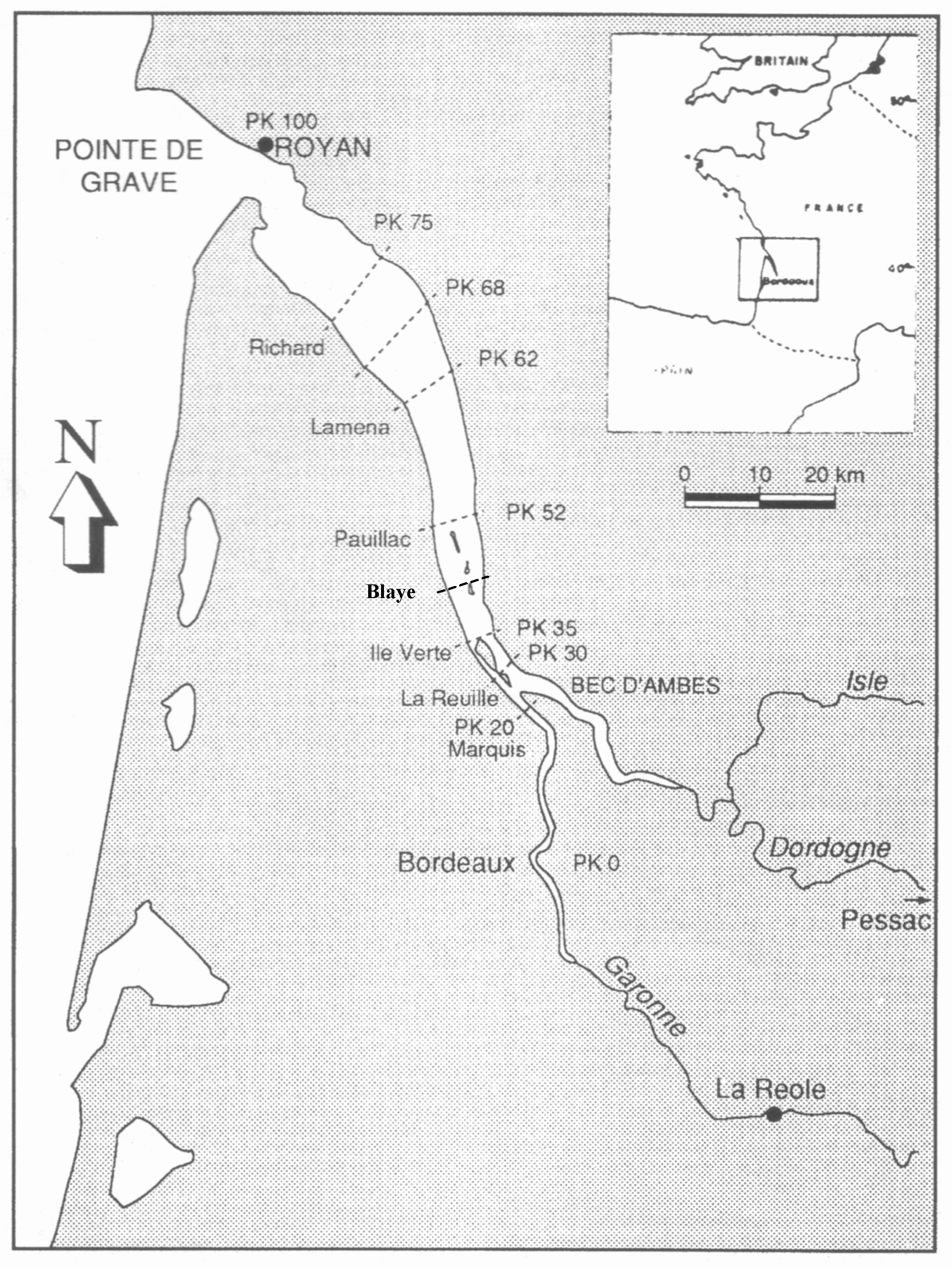
In horizontal tides, Bolle et al. [6] considered two sub-types of asymmetry: the first is related to the difference between the ebb and flood velocities, and the second is related to the duration of slack water at high and low waters. If the maximum flood velocity is higher than the maximum ebb velocity, residual mass transport will be in the flood direction. Moreover, if the slack high water is longer than the slack low water, the horizontal tide is flood-dominant. According to Friedrichs & Aubrey [7], the phase difference between M4 and M2 Δθ_M4 = (2θ_M2 − θ_M4), where θ_M2 and θ_M4 are the tidal current phases of M2 and M4, respectively, can indicate flood- or ebb-dominant states (90° < Δθ < 270° or −90° < Δθ < 90°, respectively).

Also, Bolle et al. [6] showed that asymmetry in the vertical tide will cause asymmetry in the horizontal tide. However, the relationship between vertical and horizontal tides is non-linear. Indeed, a flood-dominant vertical tide asymmetry is not necessarily associated with a flood-dominant tidal current.

The contribution of the overtide M6 to tidal asymmetry has been recently considered ([8,9,10]). Song et al. [8] showed that the asymmetry can be conveniently quantified in terms of the sample skewness, as proposed by Nidzieko [11], and reflects the asymmetry in the rise and fall of the water level. Skewness can only be generated via combinations of two or three frequency-related constituents. In such combinations, the direction of asymmetry, meaning flood- or ebb-dominant states, is determined by the relative phase (2φ_M2 − φ_M4) for the addition of two constituents or by (φ_M2 + φ_M4 − φ_M6) for triple constituents. Song et al. [10] showed that the overtide M6 can produce a double high water and a double-peak flood current. The condition to produce a double high water was given analytically between a fundamental tide, M2, and its higher harmonics (see Appendix in Song et al. [10]).

Gironde, the largest estuary in western Europe, is situated in France (Figure 1). Its total drainage area is 8 × 10⁴ km², i.e., 1/7 of the French territory. The Gironde is an estuary where the ocean tide is dominated by the semi-diurnal lunar tide (M2). The relatively restricted level of industrialisation and urban development in the southwest of France has left the Gironde as an almost undisturbed large estuary. It can be considered a valuable quasi-natural model, with a strong turbidity system due to asymmetric tides [12]. By analysing the in situ observations, Allen et al. [13] provided a synthetic description of salinity intrusion, estuarine circulation and sediment transport in the Gironde estuary. Although having addressed the tidal asymmetry characteristics of the Gironde estuary, Jouanneau et al. [8] and Allen et al. [9] did not analyse how overtides would be generated and how tidal asymmetry would affect the estuarine circulation and the saline intrusion there.

The aim of this paper, using a 3D numerical model, is to investigate (i) the spatial distribution of tidal distortion and asymmetry in the Gironde estuary in harmonically analysing tidal water levels and currents in the M2 component and M4 and M6 overtides; (ii) the estuarine circulation and the saline intrusion in the Gironde Estuary; and (iii) the reliability of the definition by Friedrichs & Aubrey [7] in predicting the nature of tidal asymmetry in the Gironde estuary.

Section 2 gives a brief description of the mathematical model. Section 3 presents the application to the Gironde estuary, the parameter settings and the calibration and verification of the model. The results and discussions are given in Section 4.

2. Study Area

The Gironde estuary is constituted by the Garonne and Dordogne rivers (Figure 1). The yearly averaged water discharge is 951 m³·s⁻¹ [12]. The tidal upper limit is observed at about 150 km upstream of the mouth, while the upper limit of salinity intrusion is at about 75 km from the estuary mouth for low river discharges and 40 km for high discharges.

According to its geographical and morphological characteristics, the Gironde estuary is divided into two, upstream and downstream, parts ([12]). The first part extends from the Bec d’Ambes to Saint-Christoly (PK68), which is nearly 30 km from the mouth (Figure 1). The morphology is complicated and characterised by a system of secondary braided channels divided by sandbanks and small islands. As a principal channel, the navigation channel is 6 to 8 m deep and flows on the left bank. The downstream part has a simple morphology forming two distinct channels separated by a succession of elongated tidal bars (Figure 2).

The navigation channel flows continuously on the left bank. In this channel, 10 km from the mouth, there is a bottom breakdown. This is where the depth falls from 10 m down to 30 m over a distance of 10 km. On the right bank, the Saintonge channel almost begins, at a depth of 6 m, 15 km from the mouth. It rejoins the navigation channel near the mouth. The bottom topography of this part is also very complex, with significant slope variations in both longitudinal and lateral directions (Figure 2). Also, the water surface width, which is uniformly about 2–3 km from Pauillac to upstream, varies from 4 km at Pauillac (60 km from the mouth) and reaches 14 km at Richard (25 km upstream from the mouth).

3. Hydrodynamic Model

3.1. Model Description

The governing equations for estuarine circulation and saline intrusion are Navier–Stokes ones using the Boussinesq approximation and the hydrostatic hypothesis, combined with transport equations for salinity (see Appendix A). A k-l-type sub-model for turbulent closure is introduced to parameterise turbulent mixing. A σ-coordinates system for the vertical is used. The governing equations are then solved by using Blumberg and Mellor’s two-successive-mode technique (for details, see [14,15,16]). The water surface elevations are determined in the external mode by solving 2D Saint-Venant equations. Then, scalar variables including the velocity components and the suspended sediment concentration are computed in the internal mode using an explicit scheme.

3.2. Computational Conditions

Besides the estuarine part, the computational domain also includes two rivers: the Garonne and the Dordogne (Figure 1). The estuarine part extends from the mouth to the confluent point at Bec d’Ambes. The river part extends from Bec d’Ambes to “La Reole” in the Garonne and to 10 km upstream of Pessac in the Dordogne. The longitudinal length of the computed domain is then nearly 160 km. Due to the tidal upper limit observed 150 km upstream of the mouth, river discharges are imposed as boundary conditions. The computational domain is discretised by a mesh of 360 × 68 × 20 in the x, y and z directions, respectively. The mesh is regular in horizontal directions with 500 m × 250 m spacing. In the vertical direction, a stretch arrangement is used to refine the mesh near the bottom. The computing time step is 30 sec, which corresponds to the maximum Courant number, Ct = 2.4. No wind is considered. The Coriolis parameter is fixed at f = 1.17 × 10⁻⁴, which corresponds to a 45° latitude. The friction stress on the bottom is calculated using Chezy’s formula, with Chezy’s coefficients varying from 50 to 80 m^−1/2·s⁻¹.

At the seaward open boundary, the observed tidal water levels are imposed. At ebb tide, no additional condition is necessary. Nevertheless, in flood tide, velocity and salinity must be additionally imposed at the offshore boundary. Therefore, the radiation method proposed by [17] and improved by [18] is used to determine the velocity component normal to the seaward open boundary. Salinity is given by a sinusoidal function, whose maximum values are observed in the Gironde mouth. At the upstream open boundaries, the discharge of the Garonne and Dordogne rivers and a salinity of 0.01 ppt corresponding to the salinity of freshwater are specified. Moreover, a radiation condition is used to determine water levels at every point. At the wall boundaries, non-slip conditions are imposed. The initial conditions for the simulations were obtained with a long simulation of 120 h.

3.3. Calibration and Verification

Until now, in the Gironde estuary, there have been several field surveys conducted. These surveys were conducted in August 2006, October–November 2009 [19] and most recently in April 2015 [20]. In general, they were performed at a few stations, poorly distributed and not sufficiently reliable for the calibration and validation of models. Strictly speaking, only two field studies are relevant for a complete validation of the model on tide-propagation, saline intrusion and sediment transport in the Gironde estuary: one was conducted from 19 to 25 May 1975 and the other from 19 to 22 May 1974 ([21]). Figure 3 illustrates the location and nature of the punctual stations used in these surveys. It is worth noting that the stations for these two field surveys were well distributed in the Gironde estuary.

As the dataset provides full data, including tidal elevations, velocity, salinity and turbidity profiles, it enables a reliable validation of the model. This justifies the use of the 1975 and 1974 data for the calibration and validation of the model, even though they are nearly 50 years old since no existing field surveys could update such information. It should be noted that the bathymetry used in the present model was measured in 1974 and 1975 (Figure 2). Therefore, the model was calibrated with measurements performed in May 1975 at six water level stations and five velocity and salinity stations, regularly spaced along the estuary. This corresponds to an average tide period. The model was then verified by measurements of water level, velocity and salinity measured during the field survey in May 1974, which corresponds to the spring tide. For both calibration and verification, a yearly averaged discharge of 700 m³·s⁻¹ was imposed for rivers at the upstream boundaries. A combination of harmonic analysis and a least-square method, LSM [22], was used to separate M2, M4 and M6, both for tidal levels and currents. Foreman and Henry [23] have shown that “meaningful results should be possible with analyses of only T = 60 h”.

Table 1. Comparison between the computed and measured water levels in M2 and the overtides M4 and M6 for the calibration step (at Richard, Lamena, Pauillac, Ile Verte, La Reuille and Marquis indicated by A1, B1, C1, D1, E1 and F1, respectively, in Figure 3).

		M2		M4		M6
		Ampli (cm)	Phase (deg)	Ampli (cm)	Phase (deg)	Ampli (cm)	Phase (deg)
Richard	Computed	222.39	21.3	15.76	64.14	55.54	174.85
	Measured	228.37	23.53	16.11	61.84	63.53	178.05
	Difference	−5.98	−2.23	−0.35	2.30	−7.99	−3.20
Lamena	Computed	246.44	11.65	11.29	66.72	61.47	161.41
	Measured	254.68	14.07	11.58	71.67	71.58	169.34
	Difference	−8.24	−2.42	−0.29	−4.95	−10.11	−7.93
Pauillac	Computed	256.89	3.02	5.05	9.34	63.8	150.16
	Measured	264.73	5.40	2.85	41.67	73.24	158.28
	Difference	−7.84	−2.38	2.2	−32.33	−9.44	−8.12
Ile Verte	Computed	253.19	11.61	14.45	25.44	62.83	132.78
	Measured	259.72	9.77	10.62	32.93	70.47	139.47
	Difference	−6.53	1.84	3.83	−7.49	−7.64	−6.69
La Reuille	Computed	255.4	15.36	14.96	22.54	64.18	129.53
	Measured	255.33	7.38	7.72	77.19	67.45	157.71
	Difference	0.07	7.98	7.24	−54.65	−3.27	−28.18
Marquis	Computed	235.58	27.15	18.92	23.56	60.8	114.98
	Measured	233.41	21.26	11.33	53.03	60.85	135.45
	Difference	2.17	5.89	7.59	−29.47	−0.05	−20.47

presents the harmonic analysis comparison between the computed and measured values for the M2 tide and the M4 and M6 overtides. It is noticed that for the M2 tide, the difference in amplitude between computed and measured values is very small: there was no difference for Marquis and La Reuille stations, and 8 cm of maximum difference was observed at Richard, Lamena and Pauillac.

The phase gap, averaged for all stations, was about 2 degrees (equivalent to 4 min approximately) with a maximum value of 8 degrees (16 min) observed at La Reuille and Marquis. Additionally, Table 1 shows that for a mean M2 tide, whose water level amplitude normally varies from 220 cm to 260 cm, the M6 contribution was more significant than that of the M4. Indeed, the water level amplitude generated by the M6 was estimated at 60–70 cm, whereas it was only 10–20 cm for the M4. Table 1 quantitatively shows small differences between the computed and measured amplitudes of the M6 at Marquis. However, it varies from 3 cm to 10 cm elsewhere.

Figure 4 shows that a reasonable agreement between the computed and measured velocity is obtained at almost all measuring stations. This agreement is more satisfactory on the surface than on the bottom. Due to the presence of fluid mud containing high concentrations near the bottom, velocity measurement by the CTD profiler could not be precise, and bottom elevation was actually not clearly determined.

Table 2. Comparison between the computed and measured values of tidal currents in M2 and the overtides M4 and M6 for the calibration step (at Richard, PK68, Lamena, Pauillac and Blaye indicated by A2, B2, C2, D2 and E2, respectively, in Figure 3).

		M2		M4		M6
		Ampli (cm/s)	Phase (deg)	Ampli (cm/s)	Phase (deg)	Ampli (cm/s)	Phase (deg)
On Surface
Richard	Computed	138.9	76.39	21.67	66.77	7.31	46.79
	Measured	107.56	54.46	25.64	63.77	18.44	132.01
	Difference	31.34	21.93	−3.97	3	−11.13	−85.22
PK68	Computed	159.55	68.19	20.93	92.99	15.39	4.95
	Measured	151.81	56.54	2.11	61.96	26.14	80.67
	Difference	7.74	11.65	18.82	31.03	−10.75	−75.72
Lamena	Computed	174.58	66.68	19.92	98.06	16.9	23.13
	Measured	164.49	45.98	9.06	178.17	19.21	127.62
	Difference	10.09	20.7	10.86	−80.11	−2.31	−104.49
Pauillac	Computed	165.03	56.35	16.18	137.46	20.54	41.73
	Measured	138.76	50.93	13.79	122.54	12.23	3.48
	Difference	26.27	5.42	2.39	14.92	8.31	38.25
Blaye	Computed	167.12	43.86	15.79	169.61	19.77	72.78
	Measured	114.13	29.13	17.73	89.36	17.14	168.9
	Difference	52.99	14.73	−1.94	80.25	2.63	−96.12
On Bottom
Richard	Computed	89.07	84.6	2.73	26.67	9.07	89.07
	Measured	55.54	87.32	2.7	75.7	6.79	55.54
	Difference	33.53	−2.72	0.03	−49.03	2.28	33.53
PK68	Computed	102.41	75.07	9.72	139.19	12.45	102.41
	Measured	108.45	47.42	14.15	131.25	11.22	108.45
	Difference	−6.04	27.65	−4.43	7.94	1.23	−6.04
Lamena	Computed	90.53	71.56	10.33	88.07	12.38	90.53
	Measured	93.99	53.07	15.51	156.43	4.81	93.99
	Difference	−3.46	18.49	−5.18	−68.36	7.57	−3.46
Pauillac	Computed	95.53	63.73	9.71	64.04	14.45	95.53
	Measured	89.4	54.5	11.83	147.34	9.08	89.4
	Difference	6.13	9.23	−2.12	−83.3	5.37	6.13
Blaye	Computed	140.5	44.53	12.59	175.69	18.83	140.5
	Measured	94.69	21.98	9.26	76.94	2.96	94.69
	Difference	45.81	22.55	3.33	98.75	15.87	45.81

gives the results of the harmonic analysis of velocity on the surface and on the bottom for M2, M4 and M6 components. Obviously, along the estuary, the contribution of overtides M4 and M6 to the velocity amplitude is nearly identical. This is about 10 cm·s⁻¹ to 20 cm·s⁻¹ over M2 tide velocity amplitudes of 100–160 cm·s⁻¹. The gap between computed and measured velocity amplitudes on average varies from 5 cm·s⁻¹ to 10 cm·s⁻¹ for all M2 tides and M4 and M6 overtides. The largest difference between calculated and measured velocity amplitudes is observed at Blaye. It is about 50 cm·s⁻¹ for the M2 tide. The Blaye station is situated between small islands near the Gironde confluent point (Figure 1), explaining this disaccord. The computing mesh includes only the largest islands because of the complex computational domain geometry. This meshing could modify the current situation in that field. In the velocity phase, the difference between computed and measured values varies from 5 degrees to 20 degrees for M2.

Figure 5 presents the excellent agreement between computed and measured salinity for the calibration step at every station. The maximum gap of 1.5 ppt for a salinity of 22 ppt was observed at Richard.

Once calibrated, the model was verified using measurements from May 1974. This was a spring tide period.

Table 3. Comparison between the computed and measured water levels in M2 and the overtides M4 and M6 for the verification step (location of PK82, PK62, PK54 and PK47 is indicated by a3, b3, c3 and d3, respectively, in Figure 3).

		M2		M4		M6
		Ampli (cm)	Phase (deg)	Ampli (cm)	Phase (deg)	Ampli (cm)	Phase (deg)
PK82	Computed	257.90	73.88	13.77	120.26	11.56	257.9
	Measured	235.95	85.35	36.85	142.12	28.25	235.95
	Difference	21.95	−11.47	−23.08	−21.86	−16.69	21.95
PK62	Computed	257.76	74.15	15.02	112.6	11.90	257.76
	Measured	233.08	86.38	36.85	142.12	28.25	233.08
	Difference	24.68	−12.23	−21.83	−29.52	−16.35	24.68
PK54	Computed	253.78	82.12	14.70	161.39	8.11	253.78
	Measured	234.96	93.30	39.58	143.62	20.49	234.96
	Difference	18.82	−11.18	−24.88	17.77	−12.38	18.82
PK47	Computed	230.06	93.54	23.48	160.53	11.53	230.06
	Measured	210.98	105.61	44.25	145.75	28.25	210.98
	Difference	19.08	−12.07	−20.77	14.78	−16.72	19.08

gives the results of the harmonic analysis of water levels for the M2 tide and the M4 and M6 overtides. The model tends to slightly over-estimate the M2 tide amplitude (a ratio of the computed amplitude of 250 cm over the measured one of 230 cm) but under-estimate the overtide amplitude (ratio of 15 cm/40 cm for M4 and 11 cm/28 cm for M6). On average, the gap between computed and measured phases is approximately 12 degrees for the M2 tide and about 22 degrees for the overtides. Figure 6 and Figure 7 present a comparison between computed and measured velocity and salinity values at four stations. Particularly, the measurements at PK82A (station a3 in Figure 3) and PK82B (station b3 in Figure 3) cover nearly 100 h and 60 h, respectively. Computational results are close to measurement ones.

4. Results and Discusion

4.1. Tidal Asymmetry

Strong tidal asymmetry in the Gironde estuary has been observed and also predicted by the present numerical model.

Table 4. Harmonic analysis of water levels for mean M2 tide and the associated M4 and M6 overtides.

	M2		M4		M6		aM4/aM2	aM6/aM2	(2φM2 − φM4) (deg)	(3φM2 − φM6) (deg)
	Ampli (cm)	Phase (deg)	Ampli (cm)	Phase (deg)	Ampli (cm)	Phase (deg)
Richard	185.21	13.73	16.16	65.84	6.23	35.28	0.09	0.03	−38.38	5.91
Lamena	202.96	4.79	11.87	70.53	8.68	32.22	0.06	0.04	−60.95	−17.86
Pauillac	210.35	3.32	4.51	20.76	14.39	81.75	0.02	0.07	−14.13	−71.80
Ile Verte	206.16	17.44	13.57	24.60	18.32	114.94	0.07	0.09	10.27	−62.63
Lareuille	207.64	21.40	14.19	21.54	17.54	123.10	0.07	0.08	21.26	−58.90
Marquis	189.17	32.84	18.27	21.78	11.89	90.94	0.10	0.06	43.91	7.60

and

Table 5. Harmonic analysis of tidal currents at mid-depth for mean M2 tide and the associated M4 and M6 overtides.

	M2		M4		M6		VM4/VM2	VM6/VM2	(2θM2 − θM4) (deg)	(3θM2 − θM6) (deg)
	Ampli (cm/s)	Phase (deg)	Ampli (cm/s)	Phase (deg)	Ampli (cm/s)	Phase (deg)
Richard	41.06	98.89	17.62	82.04	6.65	83.83	0.43	0.16	115.74	212.84
Lamena	70.07	73.27	4.40	150.60	11.65	23.00	0.06	0.17	−4.06	196.81
Pauillac	92.91	60.01	15.04	162.41	16.19	11.93	0.16	0.17	−42.38	168.11
Ile Verte	106.09	35.41	9.28	80.67	7.81	157.48	0.09	0.07	−9.84	−51.24
Lareuille	101.34	20.33	9.00	47.04	13.53	162.30	0.09	0.13	−6.38	−101.31
Marquis	77.80	14.98	10.89	15.78	24.24	172.84	0.14	0.31	14.19	−127.88

present the harmonic analysis of computed vertical (water levels) and horizontal (currents) tides obtained by using the present model for the mean tide at Richard, Lamena, Pauillac, Ile-Verte, La Reuille and Marquis, which are indicated as stations A1, B1, C1, D1, E1 and F1, respectively, in Figure 3. It is necessary to keep in mind that these locations are situated in a relatively deep zone of the navigation channel, where the average water depth is nearly 7 m, except for Richard, where the water depth is about 3.5 m.

We notice in Table 4 and Table 5 that while the amplitude of water levels of the M2 component only increased by nearly 25 cm from Richard to Pauillac, the M2 tidal current amplitude doubled its value over the same distance. This is likely due to the landward exponential decrease in estuary width. Upstream Pauillac, the tidal elevation and current amplitudes change irregularly. This may be caused by the presence of islands and confluences. Neither an increase nor decrease in the tidal elevation and current amplitude is clearly observed there. Indeed, the amplitude keeps a value nearly constant of about 208–210 cm for tidal elevations and of approximately 100 cm·s⁻¹ for currents from Pauillac to La Reuille. The amplitudes of the elevation and the velocity then decrease to 189.17 cm and 77.80 cm·s⁻¹, respectively, at Marquis. Inversely, the M4 tidal elevation amplitude decreases from 16.16 cm at Richard to a minimum value of 4.51 cm at Pauillac and then increases up to 18.27 cm at Marquis. The variation of the M6 tidal elevation amplitude has the same tendency as that of M2: the amplitude increases from Richard (6.23 cm) to Ile-Verte (18.32 cm) and then decreases to Marquis (11.89 cm).

The ratios of tidal elevation amplitude a_M4/a_M2 and a_M6/a_M2 still remain weak at less than 0.1. However, the ratios of tidal current amplitude V_M4/V_M2 and V_M6/V_M2 (where V_M2, V_M4 and V_M6 are the tidal current amplitudes of M2, M4 and M6, respectively) are especially high at Richard (0.43 and 0.16), Pauillac (0.16 and 0.17) and Marquis (0.14 and 0.31), respectively. In order to obtain an overview of the strength of horizontal tide asymmetry in the Gironde estuary, a map of isocontours of the tidal current amplitude ratios V_M4/V_M2 and V_M6/V_M2 is plotted in Figure 8 for the mean tide.

Generally, the ratio V_M4/V_M2 varies around a value between 0.1 and 0.2. This ratio becomes very large up to between 0.2 and 0.3 in the navigation channel upstream of Pauillac and especially in proximity of Richard, where it reaches a value of more than 0.40. We note that the small zone of V_M4/V_M2 values greater than 0.40 around Richard, shown in Figure 8, is a weak water depth zone. As a consequence, the term in the continuity equation should be large over there and thus promote the production of the M4 overtide via an energy transfer from M2 to M4 ([1]). The ratio of V_M6/V_M2 generally exceeds 0.15 close to the Gironde estuary and reaches 0.31 at Marquis. The increase in V_M6/V_M2 is attributed to the energy transfer from M2 to M6 via friction along the estuary. This is especially true for the islands upstream, where the estuary narrows. Clearly, the horizontal tide in the Gironde estuary would be strongly distorted by M4 and M6 overtides.

As suggested by [1], the water level–velocity diagrams describe how overtides M4 and M6 distort tidal propagation and induce tidal asymmetry. Figure 9 plots these diagrams of water levels versus mid-depth velocity at Richard, Lamena, Pauillac and Marquis. These stations are indicated as stations A1, B1, C1 and F1 in Figure 3, respectively. Clearly, the addition of M4 and M6 to M2 strongly distorts the water level–velocity ellipse. The diagrams also reveal a relatively fast clockwise shift of nearly 90° in their elliptical shape as one proceeds from Richard to Lamena. There is then a very small shift from Lamena’s further inland. This indicates a decrease in the lag between slack water and the high water level (HWL) or low water level (LWL) as a result of energy dissipation along the estuary. A maximum distortion by M4 is observed at Richard, where the ratio V_M4/V_M2 is the highest. It is 0.43 (see Table 5). As, everywhere, V_M6/V_M2 ratios are larger than 0.1, the M6 distortion is significant at all stations along the estuary. Figure 9 shows that at Richard, the combined effects of M2+M4 and M2+M4+M6 make (i) a strong ebb flow appear to shift the harmonic ebb ward at around HWL and LWL by about −0.25 m·s⁻¹ and hence (ii) increase the strength of the flood flow around slack high water by 0.20 cm·s⁻¹.

At Lamena (station B1, PK62), as the V_M6/V_M2 ratio is more significant than the V_M4/V_M2 ratio (0.17 vs. 0.06, respectively), the distortion of M2 by M2+M4+M6 is clearly distinct from that by M2+M4. The deformation by both M4 and M6 overtides at Pauillac, where the ratios V_M4/V_M2 and V_M6/V_M2 are about 0.16, modifies the strength of the maximum ebb current near LWL but does not change the strength of the peak flood current in the vicinity of HWL. At Marquis, the addition of M4 to M2 does not change the strength of both the maximum ebb and flood currents but increases HWL and LWL. As the V_M6/V_M2 ratio is approximately 0.31, distortion by M2+M4+M6 is seen as more significant at Marquis. This results in increasing the strength of the strongest tidal currents in the ebb and flood stages of the river.

Table 4 shows that relating to definition [7] and according to the phase difference Δφ = (2φ_M2 − φ_M4), the vertical tide ebbs in intensity from Richard to Pauillac and is flood-predominant from Ile-Verte to Marquis. However, according to the values of Δθ = (2θ_M2 − θ_M4) given in Table 5, the horizontal tide is ebb-predominant for most parts of the Gironde estuary except Richard. Clearly, the flood-dominant asymmetry of the vertical tide is not necessarily associated with a flood-dominant state in the horizontal tide [6].

In order to gain an overview of the horizontal tide nature in the Gironde estuary, a map of the phase differences between the M2 component and the associated overtides M4 and M6, Δθ_M4 = (2θ_M2 − θ_M4) and Δθ_M6 = (3θ_M2 − θ_M6), respectively, is plotted in Figure 10. These results are obtained from a harmonic analysis of velocities computed at mid-depth for a yearly averaged river discharge (700 m³·s⁻¹) and for the mean tide. The nature of flood- or ebb-dominant currents specified in Figure 10 has been defined following [7]. Regarding Δθ_M4 (Figure 10a), obviously only on the Maguerites bank, near the left shoreline near Richard and upstream Ile-Verte, tidal currents are flood-predominant. It is interesting to note that these areas are shallow. This is in agreement with [7], as they showed that flood dominance is associated with shoaling zones. The rest of the Gironde is dominated by ebb currents. Based on the same definition given by [7] but applied to Δθ_M6 values, Figure 10b provides a nature of a horizontal tide completely contrary to that given by Δθ_M4: flood-dominant zones previously defined according to Δθ_M4 become ebb-dependent due to Δθ_M6, and, vice versa, ebb-dominant zones defined according to Δθ_M4 become flood-dominant due to Δθ_M6. No existing study can confirm whether the definition [7] of Δθ_M4 could be applied to Δθ_M6. When the V_M6/V_M2 ratio exceeds the V_M4/V_M2 ratio, the M6 overtide decides the horizontal tide nature rather than M4. The comparison between the maps plotted in Figure 10 with maps of residual currents could give us a correct answer to these questions for the Gironde estuary.

4.2. Salinity Intrusion and Estuarine Circulation

4.2.1. Turbulence Energy

Figure 11 presents the 3D distribution of turbulence kinetic energy (TKE) intensity in the Gironde estuary at LW+3 (flood tide) and HW+3 (ebb tide). The intensity of turbulence kinetic energy (TKE) in the Gironde estuary ranges from 10⁻⁴ m²·s⁻² in proximity to the surface to 0.02 m²·s⁻² on the bottom. During ebb tides, TKE intensity is weak, with a mean value of 3.10⁻³ m²·s⁻². It reaches a maximum value of about 3.10⁻³ m²·s⁻² in the navigation channel upstream of Pauillac and in the shallow zone in proximity to the left shoreline near Richard (Figure 11b). The weak intensity of TKE reduces the vertical mixing process during ebb tides. The TKE intensity significantly increases during flood tides (Figure 11a). From LW+2 to LW+4, the TKE intensity reaches a maximum value that is greater than 0.01 m²·s⁻² upstream of Lamena and on the sandbanks such as Marguerites, Talais and Mets. This indicates that flood tides promote vertical mixings in almost the entire estuary and, in particular, on sandbanks and upstream of Lamena.

4.2.2. Saline Intrusion

Figure 12 gives the isohaline maps on three layers (on the surface, at mid-depth and on the bottom) in the Gironde estuary at different times: LW, LW+3, HW and HW+3. It is necessary to keep in mind that at LW+3 and HW+3, flows are fully in flood and ebb tide, respectively, while at LW, almost the estuary is in ebb, except for a zone that extends over 18 km from the mouth in flood. Obviously, near the mouth, the flood stage already starts at this moment. The situation is reversed at HW: the ebb stage begins in a zone extending over 24 km from the mouth, and the rest of the estuary stays in the flood stage. This explains why the saline intrusion reached the longest distance landward at HW and vice versa at LW; river freshwater pushed the farthest saltwater seaward.

Moreover, Figure 12 shows that less salty outflows have a tendency to be deflected, under the Coriolis forcing, to their right, i.e., to the right shore, and more salty inflows to the left shore along the navigation channel. As a consequence, salinity near the left shore, in particular in the navigation channel, is always higher than that near the right one in the Saintonge channel.

Table 6. Details of salinity gradients in the Gironde estuary at LW+3 (flood tide) and HW+3 (ebb tide) for the case of mean tide and of yearly averaged river discharge (700 m³·s⁻¹).

Stations (Distance from the Mouth)	Lateral Gradient of Salinity					Vertical Gradient of Salinity
	Salinity on Right Shore (ppt)	Salinity on Left Shore (ppt)	Difference (ppt)	Distance (m)	Gradient (ppt/m)	Salinity on Surface (ppt)	Salinity on Bottom (ppt)	Difference (ppt)	Depth (m)	Gradient (ppt/m)
At LW+3 (flood tide)
Pauillac (45.5 km)	Well mixed—salinity is nearly 1.50 pp everywhere in the section
Lamena (36.5 km)	6.04	4.2	1.84	5300	0.000347	2.7 9.16	6.3 9.60	3.6 0.44	7.34 10.2	0.4904 0.0431
Richard (18.5 km)	19.49	15.01	4.48	9870	0.000454	16.73 19.07	18.60 20.35	1.87 1.08	7.75 8.5	0.2412 0.1270
10 km	19.48	18.39	1.09	9800	0.000111	18.6	21.3	2.7	17	0.1588
At HW+3 (ebb tide)
Pauillac (45.5 km)	0.7	0.5	0.2	3800	0.00005	1.10	1.8	0.70	3.6	0.1944
Lamena (36.5 km)	5.03	4.76	0.27	5600	0.00048	3.4 5.12	7.4 6.5	4.0 1.38	6.0 9.0	0.6666 0.1533
Richard (18.5 km)	18.92	13.33	5.59	7810	0.00071	14.66 17.32	17.0 20.3	2.34 2.98	6.5 8.3	0.36 0.3590
10 km	20.7	18.9	1.80	9750	0.00018	19.24	23.13	3.89	5.20	0.7480

gives the numerical values of salinity gradients on the lateral and on the vertical at some locations. It shows that the lateral gradient of salinity on the surface between the right and left shores increases from Pauillac to Richard and is more important in ebb tides than in flood ones. Indeed, it varies from 0 at Pauillac to 0.00045 at Richard in flood tides versus 0.00005 to 0.00071 for the respective stations in ebb tides. At 10 km from the mouth, although the lateral gradient decreases via estuary widening, in ebb tides, it is still larger than that in flood ones (0.00018 vs. 0.00011). We note that at any time, the estuary is well mixed in the upper estuary (upstream Pauillac), where TKE is important (see Figure 11).

Figure 13 plots a 3D distribution of salinity in the Gironde estuary at different times, providing an image of vertical mixing at some crossing sections. As mentioned above, vertical mixing is more intensive in flood than in ebb tides; thus, the vertical gradient of salinity in ebb tides is larger than that in flood tides. Figure 13a shows that at LW, the moment when the ebb tide is about to finish over the estuary as a whole and river freshwater pushes saltwater farthest seaward, the vertical gradient of salinity still stays important at Richard on the Maguerites bank: the difference between salinity on the bottom and on the surface is 15 ppt and 6 ppt, respectively, over 5 m of water depth (1.8 for salinity gradient). However, in the navigation channel, the vertical gradient at the same section is less important: it is 0.79 for a difference of 6 ppt over a water depth of 7.60 m. Clearly, in the navigation channel, vertical mixing is more intensive than elsewhere.

At HW, the moment when the flood stage is about to be accomplished and saline intrusion has been fully developed and reached its upper limit in the estuary, the vertical gradient of salinity is weak: it is almost well mixed at Lamena and Pauillac, where isohalines are nearly vertical (Figure 13c). At Richard, the vertical gradient of salinity decreases to 0.466 on the Maguerites bank (4.1 ppt difference over 8.80 m water depth). Table 6 also presents the numerical values obtained from the present model for describing the variation in vertical gradients at LW+3 and LW+3 for some crossing sections.

Clearly, vertical gradients at all crossing sections in flood tides are smaller than those in ebb tides: they are 0.4904 and 0.2412 at Lamena and Richard, respectively, in flood tides in comparison with 0.6666 and 0.3600 at the same crossing sections in ebb tides. At Pauillac, in flood tides, the flow is well mixed, while in ebb tides, the vertical gradient of salinity can reach a value of 0.1944. Near the mouth, the vertical gradient of salinity in ebb tides is five times greater than that in flood tides (0.7480 vs. 0.1588 10 km from the mouth). Additional information is given in Table 6: the vertical gradients of salinity decrease in the navigation channel in both ebb and flood tides. At Lamena and Richard, in flood tides, they are, respectively, 0.0431 and 0.1270 inside the navigation channel compared with 0.4904 and 0.2412 outside. In ebb tides and at the same crossing sections, the vertical gradients of salinity inside the navigation channel are, respectively, 0.1533 and 0.3590 compared with 0.6666 and 0.3590 outside. Obviously, the vertical mixing is more intensive inside the navigation channel than outside. It is explained by the fact that inside the navigation channel, velocity is in general higher than on the outside, generates intensive TKE and then works in favour of vertical mixing inside the navigation channel.

4.2.3. Residual Circulation

The residual circulation is characterised by the upward movement of denser saline water in the lower layer and the seaward movement of fresher water in the upper layer. Figure 14 shows the map of Eulerian residual currents, superposed on iso-value contours of their intensity on the surface (a), at mid-depth (b) and on the bottom (c) for a yearly averaged river discharge (700 m³·s⁻¹) and for the mean tide. The colour scale indicates the intensity of residual currents in m·s⁻¹.

Near the bottom layer, the residual currents tend to flow upward close to the estuary even with the residual currents on the Maguerites bank, reaching a value 0.20–0.25 m·s⁻¹ stronger than that on the surface. On the mid-depth layer, there exist several eddies engendered by sandbanks (Talais, Mets and Trompeloup). The size of these eddies varies from 3 km (the eddy over the Trompeloup bank) to 10 km (that over the Talais bank), with the intensity varying from 20 to 30 cm·s⁻¹, respectively. The eddies over the Talais and Mets banks are cyclonic, and the others are anti-cyclonic. Near the mouth, rapid bottom variation affects the estuarine circulation and then the residual currents. On the other hand, the overtide M4 is a shallow water wave that reflects more or less bathymetric variation. However, the authors of [7] do not mention a clear relationship between tidal asymmetry and residual currents. We would like to compare residual currents with the flood- and ebb-predominant maps (Figure 10). The purpose of this comparison is simply to confirm or reject the hypothesis advanced by [7] concerning flood- and ebb-predominant maps. According to Friedrichs & Aubrey [7], we use the phase differences between the M2 component and the associated overtides M4 and M6, Δθ_M4 = (2θ_M2 − θ_M4) and Δθ_M6 = (3θ_M2 − θ_M6), respectively, to determine whether tidal currents are flood- or ebb-predominant. Flood- or ebb-predominant states mean that the residual current flows inlandward or seaward, respectively. It is interesting to remark that in the lower estuary extending over 40 km from the mouth, the map of Eulerian residual currents at mid-depth (Figure 14b) is in perfect agreement with the map of the horizontal tide nature defined using Δθ_M4 (Figure 10a) according to definition [7] and contradictory to the one defined using Δθ_M6 (Figure 10b). Indeed, near the mouth, Figure 10a predicts a recirculation zone, exhibited by a flood-dominant part located near the left shore and followed immediately by an ebb-dominant area situated more inside the estuary. Still, near the mouth, another recirculation zone, opposite to that previously described, is also predicted in Figure 10a. Effectively, the map of residual currents at mid-depth (Figure 14b) confirms the presence of these two recirculation zones near the mouth. In the rest of the lower estuary, and in particular, on the Maguerites bank, both Figure 10a and Figure 14b correctly indicate that this part is flood-dominant, while Figure 10b shows the opposite: the flow is ebb-dominant. The situation is reversed for the upper estuary; Figure 10b is in agreement with Figure 14b: except for inside the navigation channel where only Figure 14b shows ebb-dominant flows, both Figure 10b and Figure 14b indicate that flows are still flood-predominant close to the upper estuary, while Figure 14a indicates ebb-dominant flows in this part.

Upstream Ile-Verte, every map shows ebb-dominant flows. Therefore, we can suppose that Δθ_M4 values can be used to correctly predict tidal asymmetry. This is for zones where the V_M6/V_M2 ratio is low. In contrast, they could give an error for a high V_M6/V_M2 ratio. In this case, the M6 overtide can affect estuarine flows, and Δθ_M6 values could be used for forecasting the horizontal tide nature. This theory may be valid in this given case (i.e., yearly averaged river discharge of about 700 m³·s⁻¹ and mean tide) of the Gironde estuary. It is worthy of further research. Figure 14a shows that near the surface, residual currents flow seaward along the navigation channel. From Richard, they deviate to the right shore to exit the sea via the Saintonge channel. Inside the Saintonge Channel and at its outlet, residual currents can reach a very significant value of 0.4–0.5 m·s⁻¹. In Figure 14, the Eulerian residual circulation pattern agrees with the synthetic study conducted by [13].

5. Conclusions

This paper presents a study of tidal asymmetry, saline intrusion and residual circulation in the Gironde estuary using a fully 3D numerical model. The present model was calibrated and verified by using measurements performed during two field surveys in 1974 and 1975. These measurements correspond to mean and spring tides, respectively. The harmonic analysis of numerical results showed how the M2 component is distorted from its sinusoidal form by M4- and M6-associated overtides. The strength and nature of tide asymmetry can be determined by using the ratios V_M4/V_M2 and V_M6/V_M2 and the phase lags Δθ_M4 and Δθ_M6 (or Δφ_M4 and Δφ_M6) according to definition [7] but with caution. Indeed, the comparison between the residual circulation and the maps of phase lags proves that, for a yearly averaged river discharge (700 m³·s⁻¹) and the mean tide, the use of Δφ_M4 values could roughly correctly predict the nature of the horizontal tide for the lower part of the Gironde estuary where V_M6/V_M2 ratio is still low enough. In the upper part, where the V_M6/V_M2 ratio becomes important, it provides errors.

The use of Δθ_M6 could, under a given condition, produce fair results on the nature of horizontal tides in the upper part of the Gironde estuary. However, until now, no existing study confirmed the reliability of this use. Further research on the tide nature in relation to M4 and M6 overtides is necessary. The 3D saline distribution in the Gironde estuary was also presented under the given conditions. The variation in tidal conditions (neap or spring) and river discharges (dry or flood) will change the nature of horizontal tides and then the saline intrusion, estuarine circulation and sediment transport in the Gironde estuary. These research topics will be discussed in future articles.

References

1. Blanton, J.O.; Lin, G.; Elston, A.S. Tidal Current asymetry in shallow estuaries and tidal creeks. Cont. Shelf Res. 2002, 22, 1731–1743. [Google Scholar] [CrossRef]
2. Jay, D.A.; Smith, J.D.; Residual circulations in shallow estuaries, I.I. Weakly stratified and partially mixed. narrow estuaries. J. Geophys. Res. Oceans 1990, 95, 733–748. [Google Scholar] [CrossRef]
3. Li, M.; Zhong, L. Flood-ebb and Spring-Neap variations of mixing, stratification and circulation in Chesapeake Bay. Cont. Shelf Res. 2009, 29, 4–14. [Google Scholar] [CrossRef]
4. Moore, R.D.; Wilf, J.; Souza, A.J.; Flint, S.S. Morphological evolution of the Dee estuary, Eratern Irish Sea, UK: A tidal asymmetry approach. Geomorphology 2009, 103, 588–596. [Google Scholar] [CrossRef]
5. Zhang, Z.B.; Jeuken, M.C.J.L.; Gerritsen de Vriend, H.J.; Kornman, B.A. Morphology and asymmetry of the vertical tide in the Westerschelde estuary. Cont. Shelf Res. 2002, 22, 2599–2609. [Google Scholar] [CrossRef]
6. Bolle, A.; Wang, Z.B.; Amos, C.; De Ronde, J. The influence of changes in tidal asymmetry on residual sediment transport in the western Scheldt. Cont. Shelf Res. 2010, 30, 871–882. [Google Scholar] [CrossRef]
7. Friedrichs, C.T.; Aubrey, D.G. Non-linear Tidal Distortion in Shallow Well-Mixed Estuaries: A synthesis. Estuar. Coast. Shelf Sci. 1988, 27, 521–545. [Google Scholar] [CrossRef]
8. Song, D.; Wang, X.H.; Kiss, A.E.; Bao, X. The contribution to tidal asymmetry by different combinations of tidal constituents. J. Geophys. Res. 2011, 116, C12007. [Google Scholar] [CrossRef]
9. Song, D.; Wang, X.H.; Zhu, X.; Bao, X. Modeling studies of the far-field effects of tidal flat reclamation on tidal dynamics in the East China Seas. Estuar. Coast. Shelf Sci. 2013, 133, 147–160. [Google Scholar] [CrossRef]
10. Song, D.; Yan, Y.; Wu, W.; Diao, X.; Ding, Y.; Bao, X. Tidal distortion caused by the resonance of sexta-diurnal tides in a micromesotidal embayment. J. Geophys. Res. Oceans 2016, 121, 7599–7618. [Google Scholar] [CrossRef]
11. Nidzieko, N.J. Tidal asymmetry in estuaries with mixed semidiurnal/diurnal tides. J. Geophys. Res. 2010, 115, C08006. [Google Scholar] [CrossRef]
12. Jouanneau, J.M.; Latouche, C. The Gironde Estuary; Fuchtbauer, H., Lisitzyn, A.P., Milliman, J.D., Seibold, E., Eds.; E. Schweizerbart’sche Verlagsbuchhand: Sttugart, Germany, 1981; 115p, ISBN 978-3-510-57010-2. [Google Scholar]
13. Allen, G.P. Etude des Processus Sédimentaires Dans L’estuaire de la Gironde. Ph.D. Thesis, Université Bordeaux I, Bordeaux, France, 1972; 314p. (In French). [Google Scholar]
14. Blumberg, A.F.; Mellor, G.L. A description of a three-dimensional coastal circulation model. In Three-Dimensional Coastal Ocean Models 4; Coastal and Estuarine Sciences 4; AGU: Washington, DC, USA, 1987; 16p. [Google Scholar] [CrossRef]
15. Nguyen, K.D.; Ouahsine, A. A Numerical Study on the Tidal Circulation in the Strait of Dover. J. Waterw. Port Coast. Ocean Eng. ASCE 1997, 123, 8–15. [Google Scholar] [CrossRef]
16. Uh Zapata, M.; Zhang, W.; Pham-Van-Bang, D.; Nguyen, K.D. A parallel second-order unstructured finite volume method for 3D free-surface flows using a σ coordinate. Comput. Fluids 2019, 190, 15–29. [Google Scholar] [CrossRef]
17. Orlanski, I. A Simple Boundary Condition for Unbounded Hyperbolic Flows. J. Comput. Phys. 1976, 21, 251–269. [Google Scholar] [CrossRef]
18. Blumberg, A.F.; Kantha, L.H. Open boundary Condition for Circulation Model. J. Hydraul. Eng. 1985, 111, 237–255. [Google Scholar] [CrossRef]
19. Huybrechts, N.; Villaret, C.; Lyard, F. Optimized Predictive Two-Dimensional Hydrodynamic Model of the Gironde Estuary in France. J. Waterw. Port Coast. Ocean Eng. 2012, 138, 312–322. [Google Scholar] [CrossRef]
20. Ross, L.; Valle-Levinson, A.; Sottolichio, A.; Huybrechts, N. Lateral variability of subtidal flow at the mid-reaches of a macrotidal estuary. J. Geophys. Res. Oceans 2017, 122, 7651–7673. [Google Scholar] [CrossRef]
21. Li, Z.H.; Nguyen, K.D.; Brun-Cottan, J.C.; Martin, J.M. Numerical simulation Numerical model of the turbidity maximum transport in the Gironde estuary (France). Oceanol. Acta 1994, 17, 479–500. [Google Scholar]
22. Venedikov, A.P.; Arnoso, J.; Vieira, R. Program VAV/2000 for tidal analysis of unevenly spaced data with irregular drift and colored noise. J. Geod. Soc. Jpn. 2001, 47, 281–286. [Google Scholar]
23. Foreman, M.G.; Henry, R.F. The harmonic analysis of tidal model time series. Adv. Water Resour. 1989, 12, 109–120. [Google Scholar] [CrossRef]
24. Hieu, H.M. Modélisation de la turbulence: Ses aspect physiques et son impact sur la simulation numérique des écoulements réel. In Proceedings of the 11ème Congrés Français de Mécanique, Lille, France, 6–10 September 1993. (In French). [Google Scholar]
25. Nihoul, J.C.J. A 3D general marine circulation model in a remote sensing perpective. Ann. Geophsicae 1984, 2, 433–442. [Google Scholar]
26. Escudier, M.P. The Distribution of Mixing Length in Turbulent Flow Near Walls, Imperial College, Heat Transfer Section, Report TWF/TN/1; Cambridge University Press: Cambridge, UK, 1966. [Google Scholar]
27. Phillips, N.A. A coordinate system having some special advantages for numerical forecasting. J. Metorol. 1957, 14, 184–185. [Google Scholar] [CrossRef]
28. Chorin, A.J. Numerical solution of the Navier-Stokes equations. Math. Comput. 1968, 22, 745–762. [Google Scholar] [CrossRef]
29. Nguyen, K.D.; Martin, J.M. A two-dimensional fourth-order simulation for scalar trasnport in estuaries and coastal seas. J. Estuar. Coast. Shelf Sci. 1988, 27, 263–281. [Google Scholar] [CrossRef]
Figure 1. Location map of the Gironde estuary (France) showing the sampling section (PK: kilometric point, downstream from Bordeaux, [9]).
Water 15 04042 g001
Figure 2. Bathymetry of the Gironde estuary (the sandbanks are reported in the figure).
Water 15 04042 g002
Figure 3. Location of the measure stations in the field surveys from May 1975 (for calibration) and May 1974 (for verification).
Water 15 04042 g003
Figure 4. Comparison between computed and measured velocity on surface and on bottom for calibration (mean tide, yearly average discharge ≈ 700 m3·s−1).
Water 15 04042 g004
Figure 5. Comparison between computed and measured values of salinity on surface and on bottom for calibration (mean tide, yearly average discharge ≈ 700 m3·s−1).
Water 15 04042 g005
Figure 6. Comparison between the computed and measured values of velocity on surface and on bottom for verification (spring tide, yearly averaged river discharge ≈ 700 m3·s−1).
Water 15 04042 g006
Figure 7. Comparison between the computed and measured salinity (ppt) on surface and on bottom for verification (spring tide, yearly averaged river discharge ≈ 700 m3·s−1).
Water 15 04042 g007
Figure 8. Isocontours of tidal current amplitude ratios VM6/VM2 (upper) and VM4/VM2 (lower) computed at mid-depth for a yearly averaged river discharge (≈700 m3·s−1) and for the mean tide in the Gironde estuary.
Water 15 04042 g008
Figure 9. Water level-velocity diagrams at the mid-depth at station Richard, Lamena, Pauillac and Marquis for a yearly averaged river discharge (≈700 m3·s−1) and the mean tide.
Water 15 04042 g009
Figure 10. Isocontours of phase lag (a) ΔθM4 = (2θM2 − θM4) and (b) ΔθM6 = (3θM2 − θM6) in the Gironde estuary, computed at mid-depth for a yearly averaged discharge (≈700 m3·s−1) and for the mean tide. F denotes flood-dominant zones, and E denotes ebb-dominant ones.
Water 15 04042 g010
Figure 11. Three-dimensional distribution of turbulent kinetic energy at LW+3 (a) and HW+3 (b) in the navigation channel (discharge ≈ 700 m3·s−1, mean tide).
Water 15 04042 g011
Figure 12. Isohaline maps for different layers (on surface (a), mid-depth (b) and on bottom (c)) at LW, LW+3 (flood tide), HW and HW+3 (ebb tide) (river discharge ≈ 700 m3·s−1, mean tide).
Water 15 04042 g012aWater 15 04042 g012b
Figure 13. Three-dimensional distribution of salinity at LW (a), LW+3 (b), HW (c) and HW+3 (d) in the Gironde estuary (river discharge ≈ 700 m3·s−1, mean tide).
Water 15 04042 g013aWater 15 04042 g013b
Figure 14. Five-day Eulerian residual currents on surface (a), at mid-depth (b) and on bottom (c) for a yearly averaged river discharge ≈700 m3·s−1 and mean tide under the effect of sandbanks: (A) Talais, (B) Mets, (C) Trompeloup1 and Trompeloup2. Colour scale shows the intensity in m·s−1 of residual currents.
Water 15 04042 g014