Review

Understanding How Reservoir Operations Influence Methane Emissions: A Conceptual Model

by
Henriette I. Jager
*,
Rachel M. Pilla
,
Carly H. Hansen
,
Paul G. Matson
,
Bilal Iftikhar
and
Natalie A. Griffiths
Oak Ridge National Laboratory, Oak Ridge, TN 37831-6038, USA
*
Author to whom correspondence should be addressed.
Current address: Irrigation Department, Government of Punjab, Lahore 54840, Punjab, Pakistan.
Water 2023, 15(23), 4112; https://doi.org/10.3390/w15234112
Submission received: 4 October 2023 / Revised: 9 November 2023 / Accepted: 11 November 2023 / Published: 27 November 2023

Abstract

:
Because methane is a potent greenhouse gas (GHG), understanding controls on methane emissions from reservoirs is an important goal. Yet, reservoirs are complex ecosystems, and mechanisms by which reservoir operations influence methane emissions are poorly understood. In part, this is because emissions occur in ‘hot spots’ and ‘hot moments’. In this study, we address three research questions, ‘What are the causal pathways through which reservoir operations and resulting water level fluctuations (WLF) influence methane emissions?’; ‘How do influences from WLF differ for seasonal drawdown and diurnal hydropeaking operations?’; and ‘How does understanding causal pathways inform practical options for mitigation?’. A graphical conceptual model is presented that links WLF in reservoirs to methane emissions via four causal pathways: (1) water-column mixing (2) drying–rewetting cycles, (3) sediment delivery and redistribution, and (4) littoral vegetation. We review what is known about linkages for WLF at seasonal and diurnal resolutions generate research questions, and hypothesize strategies for moderating methane emissions by interrupting each causal pathway. Those related to flow management involve basin-scale management of tributary flows, seasonal timing of hydropeaking (pathway #1), timing and rates of drawdown (pathway #2). In addition, we describe how sediment (pathway #3) and vegetation management (pathway #4) could interrupt linkages between WLF and emissions. We demonstrate the strength of conceptual modeling as a tool for generating plausible hypotheses and suggesting mitigation strategies. Future research is needed to develop simpler models at appropriate timescales that can be validated and used to manage flow releases from reservoirs.

1. Introduction

Freshwater networks return a substantial proportion of terrestrial carbon to the atmosphere as methane [1], accounting for half of global emissions [1]. Knowledge about the effects of water-level fluctuations on methane comes from rivers [2,3], lakes [4], and wetlands [5]. In particular, rewetting of river floodplains during warm periods is associated with high methane emissions [3].
Reservoirs are now a part of freshwater networks. A subset of these has structures to control water level fluctuations, which has implications for greenhouse gas emissions. Relationships between reservoir operations and greenhouse-gas (GHG) emissions are complex and poorly understood. As a renewable energy source, hydropower displaces fossil fuels and adds grid stability by filling in for other renewables. However, reservoirs that support hydropower generation also tend to have large surface areas and can emit significant amounts of methane [6,7,8]. Reconciling the costs and benefits of hydropower generation, particularly in terms of its carbon footprint [9], is crucial to meet sustainable energy production goals.
Reservoirs are complex systems with carbon dynamics influenced by both natural and anthropogenic factors. The initial inundation and subsequent decay of terrestrial organic matter typically occurs over the first decade of a reservoir’s life [10,11]. In older reservoirs, methane production is supported by the decomposition of terrestrial organic matter from upstream inputs and the surrounding watershed, as well as by in situ algal production. Methane emissions have been described as sporadic, often occurring as ‘hot moments’ during which conditions are right for the gas to be produced and emitted [12,13]. The timing of hot moments is influenced by seasonal patterns of flows, carbon and nutrient inputs [14], water-column stratification [15], and water-level fluctuations [16,17,18,19].
Fewer than 3% of reservoirs in the US support hydropower [20]. For this subset, GHG emissions are mediated by the timing and amounts of water released, which control reservoir water-level fluctuations (WLF) at seasonal and diurnal time scales. At a seasonal timescale, water levels in storage reservoirs used for flood control are drawn down by releasing water in the fall. This ensures that enough storage capacity is available in the reservoir to store water from spring high flows to fulfill water demand during drier summer conditions. Some hydropower reservoirs are operated to release more water when energy prices are high. The increased release of water during times of peak, unmet electricity demand results in diurnal fluctuations in water level (‘hydropeaking’) [21]. A review of 33% of US hydropower plants found that roughly 40% of them released flows with significant sub-daily variation during at least part of the year [22]. As variable renewables (solar and wind power) are being added to the grid, twice-daily hydropeaking is becoming more frequent to compensate when variable renewables are not generating (‘double peaking’) [23]. Dams operated in peaking mode either have more storage than non-peaking projects or, for run-of-river reservoirs with short residence times, they pass stored water from upstream storage reservoirs releasing fluctuating flows [22]. Most run-of-river hydroelectric reservoirs are required to balance inflows and outflows on a daily timescale and can therefore experience significant within-day fluctuations in water level. Both seasonal and diurnal fluctuations in reservoir water level can affect methane emissions through various mechanisms, including changes in hydrostatic pressure [24], mixing dynamics [25], and drying–rewetting cycles [26].
The goal of this study is to improve our understanding of processes linking reservoir operations to carbon dynamics leading to methane emissions. Key questions addressed include:
  • What are the causal pathways through which reservoir operations and resulting WLF influence methane emissions?
  • How do influences from WLF differ for seasonal drawdown and diurnal hydropeaking operations?
  • How does understanding causal pathways inform practical options for mitigation (i.e., reducing methane emissions via scheduled releases)?
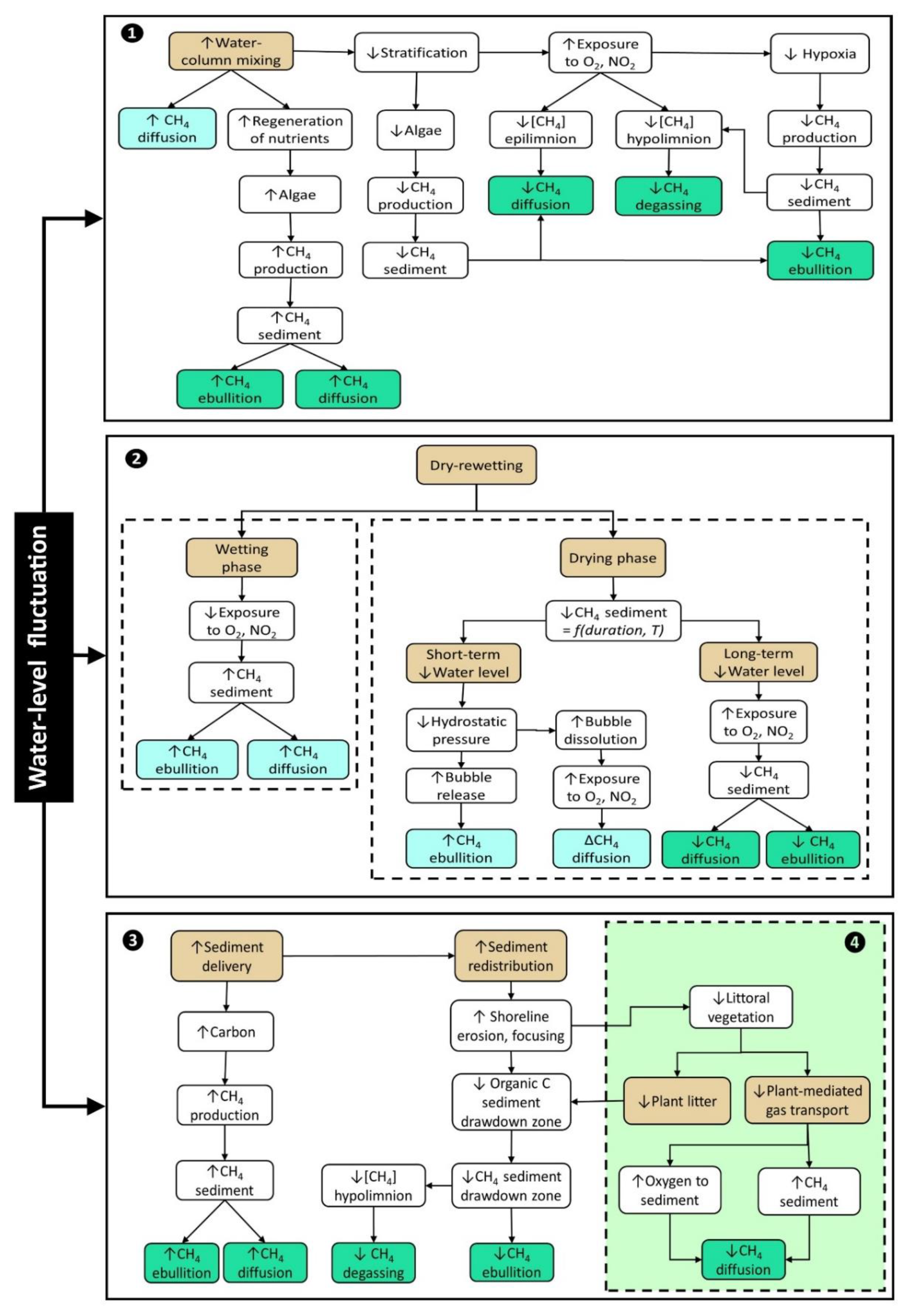
We developed a conceptual model to clarify the causal linkages between WLF (specifically those associated with hydropower operations) and methane emissions. Conceptual ecological models (also called ‘causal models’) are graphic representations (diagrams) with a written description of predicted relationships between anthropogenic stressors and environmental outcomes. They are used as a first step in ecological risk analysis [27]. The diagrams represent hypotheses about causal linkages between the management actions of interest (e.g., reservoir operation) and outcomes (e.g., methane emissions). Although they are qualitative, causal models can be used as a first step in developing quantitative models, such as structural equation models [28] or dynamic systems models [29]. We also review equations associated with the system.

2. Conceptual Model

A review of the recent literature on GHG emissions from reservoirs identified key processes and factors that can aid in predicting emissions [9]. Here, we update and augment that review to understand key predictors to consider in future when constructing indicators of methane emissions. Our expanded review includes information from other ecosystems, such as wetlands and floodplains, that are relevant to understanding linkages between WLF and methane emissions. Based on our review and understanding of methane dynamics, we produced a graphical conceptual model of causal linkages between reservoir operations and methane emissions from reservoirs. We organized our review of methane production and transport to the atmosphere around causal pathways (drying–rewetting, sediment delivery and redistribution, plant-mediated emissions, mixing and stratification, turbine withdrawal) with distinctions made between two temporal scales (seasonal dynamics, diurnal hydropeaking). This should be seen as a strawman and used as the basis for further refinement. For each causal pathway, we report relevant equations and describe which methane generation and emission processes are most influenced by each pathway.
Our conceptual model seeks to understand the causal pathways through which methane emissions are linked to WLF at different time scales (Figure 1). Three causal pathways take place mainly in the littoral zone (drying–rewetting, sediment delivery and redistribution, and plant-mediated emissions), whereas mixing mainly takes place in the limnetic zone along with turbine withdrawal. First, WLF can alter the mixing dynamics of reservoirs (causal pathway #1 in Figure 1). WLF can disrupt thermal stratification and vertical oxygen gradients that control oxygen levels below the thermocline and conditions that promote methane production. The second causal pathway identified here is mediated by drying and rewetting of littoral sediments. In the middle box of Figure 1, we distinguish between the dominant effects of WLF during the wetting phase and the drying phase (Figure 2). We also distinguish diurnal (short-term) and seasonal (long-term) effects of drying, where we assume that drawdown and refill represent slower, longer-term changes in water elevation than hydropeaking. Third, WLF can deliver sediment from floodplains and cause resuspension and focusing of sediment in deeper areas of the reservoir [30]. This should lower the potential for methane emissions during rewetting cycles, which can become limited by availability of organic carbon in shallower areas [31,32]. Fourth, alternate drying and rewetting of sediments can result in a loss of littoral vegetation as few plant species are adapted to extended periods of dry and wet soils or sediment erosion. Reduced vegetation reduces the potential for plant-mediated methane transport. Each of these pathways is described in more detail in the sections below.
In addition to conceptual modeling, we diagramed a simplified systems model with methane pools and fluxes (Figure 2). Although a complete systems model is beyond our scope, we present equations corresponding with the system depicted in Figure 2 for amounts of methane (masses) in three pools, sediment, C H 4 ( t ) s e d , deep, hypolimnetic water,   C H 4 ( t ) d e e p , and the epilimnion,   C H 4 ( t ) t o p (Table S1, Equations (S1)–(S3)). We refer to mass flows as ‘fluxes’ for convenience, and many parameters are rates representing fluxes as a proportion of a donor pool’s mass (Table 1). The flux of methane produced in sediment P ( t ) s e d adds to the pool of methane in sediment ,   C H 4 ( t ) s e d , which can leave the pool in three ways, via (1) sediment diffusion at rate, D f t s e d , (2) bubble release from the sediment at rate B r t , or (3) as a flux to the atmosphere through plants, A p [33] (Figure 2). Rates depend on temperature and other factors not explicitly included. Variables used in the equations are defined in Table 1.
Dissolved methane concentration in the hypolimnion, C H 4 d e e p , increases via diffusion of methane from sediment at rate D f s e d , and dissolution of methane bubbles from pool C H 4 b u b at rate Bd. The deep-water pool loses methane to oxidation, Ox, diffusion into the surface layer, Dfdeep, and degassing due to turbine passage, Tb [Table S1, Equation (S2)]. Degassing depends indirectly on the production of methane, Psed, in sediment and competing losses from sediment via transport through plant aerenchyma tissue, Ap. In a spatial model representing methane dynamics in littoral areas separately from the limnetic/open-water zone, one could assume that Ap is negligible in the limnetic zone.
Ebullition is an important pathway whereby methane protected inside bubbles avoids oxidation during their ascent through the water column. Ebullition is influenced by the sum of changes in atmospheric and hydrostatic pressure [34]. Decreases in reservoir elevation reduce hydrostatic pressure, ∆Pa, experienced by littoral sediments, which can produce a short-term pulse of methane via ebullition [16,17,35,36]. When the rate of methane production in sediment exceeds the rate at which it can diffuse into the water column, bubbles form and ebullition takes place [37]. The rate of bubble release from sediment, Br, is controlled by temperature and hydrostatic pressure [see [38], Equation (S5)]. One study reported that methane ebullition followed an exponential increase with decreasing pressure as water levels dropped from 0.2 to 1.3 m [39]. Conversely, ebullition diminished as water levels rose [39].
The pool of methane contained in bubbles, C H 4 ( t ) b u b , is incremented by methane released from sediment and decremented by methane lost to bubble dissolution or ebullition flux from the surface (Figure 2). The flux of methane bubbles released from sediment, Br(t), depends on an upper methane concentration threshold [Table S1, Equation (S7)], which, in turn depends on pressure, bubble volume, and temperature [38,40]. Because bubbles form and release only at low ambient hydrostatic pressures, models that consider pressure predict ebullition events better than those relying on sediment methane concentration alone [38,41]. In addition to depth-related hydrostatic pressure, ebullition increases with increasing temperature and decreases with increasing wind speed [42].
Methane in bubbles dissolve at rate Bd, resulting in a lower ebullitive emission by the time the bubbles reach the water’s surface and increased concentrations of dissolved methane (Figure 1, pathway #2; Figure 2). Bubble dissolution, B d t [Table S1, Equation (S8)], depends on bubble depth at release and dissolution rate while traveling through the water column and other factors, such as bubble size [43]. The distribution of initial bubble sizes is an important factor because bubble size is proportional to bubble rise velocity [44]. Bubble size, in turn, is determined by sediment characteristics, decreasing from clay to sand to silt [45]. Thus, WLF may influence bubble size through grain size distributions, an outcome of sediment redistribution (Section 2.3).
When methane bubbles dissolve, aerobic methanotrophs in the water column incorporate carbon into microbial biomass in the oxycline [46]. This can prevent a significant fraction of dissolved methane from reaching the atmosphere [46]. This process has been represented differently by different models. For example, the monthly Reservoir Methane Emissions model (ResME) represents oxidation in oxic portions of sediment layers as a function of bubble dissolution, but it does not represent oxidation of dissolved methane in the water column [47]. ResME describes bubble dissolution from the point of bubble release from sediment as a function of average reservoir depth. A 60-m reservoir depth limit [Table S1, Equation (S8)] is based on the inference that 4–6-mm diameter bubbles will completely dissolve after rising through Dox = 60 m of water [48]. This depth may vary among reservoirs. For example, a model of emissions from a well-studied reservoir in Israel estimated that 60% of simulated methane in bubbles released from sediment reached the atmosphere [49], even though methane was almost-completely oxidized. ResME assumes that the daily fraction of methane in bubbles that dissolves, Bdmax, is less than 20% because some methane produced in littoral sediments will still reach the atmosphere, even in deep reservoirs. The remainder of methane produced is oxidized after bubbles dissolve [47]. Another model, the GHG Reservoir (G-Res) model represents oxidation of dissolved methane, but not bubble dissolution [17].
Model assumptions about depth-dependent oxidation rates in the water column can be supported by isotopic depth profiles of methane [14,46]. Ideally, depth dependence of oxidation should reflect both the increased availability of dissolved oxygen to methanotrophs and the decreased dissolution of methane bubbles in shallower water. Consistent with our two-layer conceptual model (Figure 2), methane in the surface layer is incremented by diffusion from deeper layers and decremented by ebullitive and diffusive surface fluxes to the atmosphere (Figure 2). Diffusive methane emission, D f t o p , emanating from the pool of methane in the epilimnion, C H 4 t t o p , can be estimated by subtracting the proportion oxidized, O x t [Table S1, Equation (S6)], and adding methane from bubble dissolution, which occurs at rate B d t , a function of water depth [Table S1, Equation (S8)]. Oxidation within sediment (under certain conditions), bubble release from sediment to deep water, and subsequent dissolution and oxidation in the water column, would be represented as separate processes.

2.1. Water-Column Mixing

WLF induces mixing (pathway #1 in Figure 1), which has different short- and long-term effects on methane production and emission. Typically, turnover events are seen as producing pulses of diffusive emissions in the short term, but oxygenation of deep waters reduces methane concentrations and decreases methane emissions over the long term. For example, in the short-term, diurnal interruptions of stratification in Iron Gate I, a relatively shallow run-of-river reservoir on the Danube River, enabled diffusion of methane in the water column [50]. Advective mixing also influences oxidative methanotrophy by controlling where the supply of oxygen, dissolved methane, and methanotrophs in the water column [46] coincide with thermal conditions that favor methanotrophy.
The proportion of the world’s largest reservoirs that stratify is not well known [51], with a recent estimate of 70% based on reservoir morphometry [52]. Both the timing and depth of water releases from reservoirs influence mixing and stratification, especially when the change in volume associated with WLF is a large proportion of reservoir volume at full pool [53]. Selective withdrawal from deep water layers shortens the period of summer stratification by depleting cold water in the hypolimnion and decreasing the stability of the water column [54]. Generally, faster-flowing waters (those with shorter residence times) do not stratify because there is no opportunity for surface heating to produce depth gradients as it does in more stagnant waters. The source of carbon fueling methane production also depends on residence time. In reservoirs with short residence times, methane production is linked to allochthonous carbon, whereas methane production in reservoirs with longer residence times is better predicted by autochthonous carbon (e.g., algae) [47].
Degassing, i.e., emissions from water flowing through turbines, are a poorly quantified, component of reservoirs’ carbon footprint of particular relevance to hydropower [55]. Estimates vary widely. One estimate based on the G-Res model suggested that degassing accounts for 31–52% of global methane fluxes from reservoirs [8]. This estimate is likely high because it assumed that all reservoirs stratify and that all flows in reservoirs that support hydropower are drawn from methane-rich hypolimnetic water. Another study of US reservoirs did not find degassing to be the dominant emissions pathway [55]. Degassing is strongly dependent on methane concentration and flow; as water passes through the intakes (or turbines in the case of hydropower), hydrostatic pressure decreases and dissolved methane is released immediately downstream of the discharge [56].
Lima, Ramos, Bambace and Rosa [56] modelled degassing as a fraction, ф, of methane passing through turbines. For reservoirs with bottom withdrawals, degassing is proportional to the concentration of methane in the hypolimnion, [ C H 4 ] ( t ) d e e p . We refined the equation to represent the fraction of flow, Q(t), passing through turbines on day t, by incorporating fractional turbine flow, Tf(t), which ranges from zero (no generation, 100% spill) to one (100% generation, no spill) [Table S1, Equation (S10))].
Methane emissions from managed reservoirs are influenced by the timing of water releases (i.e., reservoir operation), the depth of intakes, and the proportion of flow passed through turbines versus non-turbine routes, such as bypass structures and spill. Spillways may only be active for part of the year to cope with seasonal precipitation or snowmelt events [56] or to provide downstream fish passage [24]. To integrate reservoir operations in a way that is consistent with our conceptual model, turbine degassing can be represented by integrating Tf(t) over time, where [ C H 4 ] ( t ) d e e p is a function of antecedent hypoxic conditions [Table S1, Equation (S1) or Equation (S2)]. Note also that methane removal through turbines from the deep-water layer decreases the pool of hypolimnetic methane when withdrawals exceed production (Figure 2). In addition to degassing, elevated methane levels in tailwaters can lead to high downstream emissions that decays with distance downstream [57,58].

2.1.1. Seasonal Dynamics (Stratification, Turnover, and Drawdown)

Typical seasonal patterns in stratification and WLF that influence methane emissions are depicted in Figure 3. In temperate regions, deeper reservoirs become thermally stratified as the gradient between warmer surface waters and colder, denser bottom waters increases in late spring. This leads to a separation of oxygenated water above the thermocline and less-oxygenated water below, where resupply of oxygen to deeper waters via wind-driven mixing or photosynthesis is negligible. Inverse stratification can also occur after ice-over in northern latitudes. During fall turnover, surface temperatures decrease causing shallower waters to reach similar densities as deeper waters, at which point the water is less resistant to advective forcings (e.g., wind, flow) that induce mixing (Box 3 in Figure 3). Similarly, in reservoirs that freeze over, mixing events occur after ice-off in spring (left-most Box 5 in Figure 3).
Seasonal dynamics of methane emissions differ significantly in reservoirs that stratify and those that do not, and for those that stratify, reservoir release patterns can have important effects. Typical seasonal patterns with reservoir drawdown lead to lower water releases in summer, which decreases mixing and increases surface heating and water-column stability (i.e., stratification) [60]. While a reservoir is stratified, methane concentrations increase in the hypolimnion, controlled by redox dynamics and temperature. During stratification, methane build-up in the hypolimnion has been observed across a range of reservoir types in the US [16,17,24]. If we assume negligible oxidation occurs in the deep, anoxic portion of the water column, methane accumulation in the hypolimnion can be modeled by adding daily methane diffusion, Dfsed from the anoxic sediment to the deep-water pool and bubble dissolution below the oxycline and subtracting daily amounts removed by turbine degassing, Tb [Equation (1)].
C H 4 T m i x d e e p = C H 4 T s d e e p + t = T s + 1 T m i x Δ C H 4 t d e e p ,  
where
Δ C H 4 t d e e p = C H 4 t d e e p 1 T b t + D f t s e d C H 4 t s e d + B d t C H 4 t b u b
T m i x = day   of fall overturn ,
t s = day   of stratification , onset
Any significant mixing events during the stratification period would result in oxidation of a proportion, pM, of CH4deep that could be modeled as an increasing function of the magnitude of WLF. Equation (1) can be generalized by defining R ‘runs’ of dates with anoxic conditions, r = 1 to R, where the first day of fall turnover occurs at the end of the last, Rth, run, i.e., Tmix = tm(R). Let the start of the stratification (or restratification) period r be ts(r) and the end of the stratified period r be tm(r). Cumulative methane in the deep layer can then be represented by Equation (2).
C H 4 T m i x d e e p = r = 1 t m r p M r t = t s r t m r 1 Δ C H 4 t d e e p ,
where
t m r = day   of rth mixing event
t s = day   of   [ re ] stratification
Fall turnover is considered a potential ‘hot moment’ for emissions [61]. Methane generated in the sediments and water column of the hypolimnion is trapped in deep water during stratification. Later, the portion of this accumulated methane emitted via diffusion and ebullition pathways can represent a significant fraction of reservoir emissions, especially as a pulse of emissions during turnover [62]. In one Virginia reservoir, ebullition rates peaked just before fall turnover, whereas methane diffusion peaked during turnover [42]. These turnover pulses may be localized hot spots; for example, cold temperatures and replenished dissolved oxygen at the time of fall turnover may depress methane production in shallow areas [14]. Diffusion of some accumulated methane across the thermocline may occur prior to turnover, especially when concentrations below the thermocline are high [14]. Often, a fraction of methane is not oxidized during fall mixing and remains in the dissolved methane pool. The remaining fraction varies (e.g., a reasonable range may be from 50 to 90% [47]) depending on reservoir geomorphology. The opportunity for oxidation is greater in deep hydropower reservoirs, preventing 90% [62] to 99% [49] of dissolved methane in the hypolimnion from reaching the atmosphere via diffusion.
Like emissions during fall turnover, emissions of methane accumulated under ice may peak after spring ice-off. For example, spring pulse emissions were reported from the surface waters of deep boreal reservoirs [63]. In warmer climates, extended anoxic conditions and methane storage during summer produce larger emissions during autumn overturn, whereas in cooler climates, larger pulses are produced during spring turnover [61]. However, methane generation in winter is likely lower due to lower water temperatures.
Superimposed on natural seasonal patterns are the effects of reservoir operations. A large majority of US reservoirs experience at least one annual drawdown > 0.5 m [17]. This typically occurs in autumn in snowmelt-dominated and many rainfall-dominated catchments of the US. Because methane builds up in the hypolimnion during stratification, the timing of artificial reservoir drawdown relative to natural seasonal patterns is important. Several studies have documented increases in ebullitive methane emissions in stratified reservoirs following drawdown prior to fall turnover. Drawdown increases methane ebullition (pathway #2 in Figure 1) by decreasing hydrostatic pressure, which increases bubble formation and release [17]. For example, in Harsha Lake, a eutrophic Midwestern US reservoir, ebullitive methane emissions increased substantially following an experimental fast drawdown in September, especially at shallower sites [16]. Harsha Lake stratifies from mid-May to mid-October [16]. Because the pulse was short-lived, it constituted only 3% of emissions measured over a 7-month period [16]. Another study of two reservoirs in the Pacific Northwest produced different results. In these reservoirs, that stratified from June to October, ebullitive emissions during an August drawdown [64], accounted for 90% of annual methane emissions [17]. In one reservoir, the annual mass of dissolved methane, C H 4 ( t ) d e e p ,   was modeled [Equation (3)] as a function of duration of antecedent hypoxic conditions and a variable indicating whether water was being spilled from the epilimnion to achieve drawdown [24].
C H 4 t + 1 d e e p = α + β Year + γ if drawdown 0 otherwise
Drawdown was found to be a significant predictor in the best-performing models. Differences among years were better explained by water-column stability than by algal production [24]. In years with higher water-column stability (i.e., high resistance to mechanical mixing), oxidants in the water column were depleted and methane produced in sediments was able to accumulate in the hypolimnion without being oxidized [24]. However, we note that unlike the reservoirs studied by Deemer and Harrison, most hydropower reservoirs achieve drawdown through hypolimnetic withdrawals. Drawdown is likely to have different effects on upstream emissions in reservoirs with hypolimnetic withdrawals because methane accumulated in the hypolimnion is removed and instead contributes to downstream degassing emissions.
Methane degassing is directly related to flow rates and partial pressure of methane in the reservoir at the intake depth, which are both influenced by seasonal release patterns [65]. Specifically, hypolimnetic releases from hydropower reservoirs promote thermal mixing and disrupt stratification [66,67]. Operations that promote mixing will lower degassing emissions by bringing oxygenated water down to the sediments. Kemenes et al. [68] reported lower methane degassing fluxes from a Brazilian reservoir during the rainy season when stratification was weak and hypolimnetic methane concentrations were low. Low methane degassing fluxes were also reported from several run-of-river reservoirs in the Columbia Basin, US from summer through fall, possibly because they did not stratify [69].

2.1.2. Diurnal Hydropeaking

According to our conceptual model, hydropeaking can have positive or negative effects on methane emissions depending on whether the dominant mechanism is reduced hydrostatic pressure (leading to increased ebullition, pathway #2 in Figure 1) in the drawdown zone or water column mixing (leading to lower methane production) (pathway #1 in Figure 1). Positive effects on ebullition rates mediated by reduced hydrostatic pressure as a result of hydropeaking were reported by one study of reservoirs in the Pacific Northwest [17]. The study compared time series of methane concentrations and emissions in two cascade reservoirs, Keno and J.C. Boyle. Keno feeds into J.C. Boyle, which is a peaking reservoir. Diurnal fluctuations in J.C. Boyle produced pulses of methane ebullition that increased emissions by a factor of 3.5 relative to Keno [17].
On the other hand, over a longer time horizon, volatility in water levels might decrease emissions for several reasons. Repeated ebullition events could deplete sediment methane faster than it is produced so that integrated emissions over time might not be higher under peaking operations, especially in reservoirs with low sediment storage capacity for methane [17].
Secondly, hydropeaking shortens the period of stratification in summer and fall [70,71]. For example, in the Three-Gorges reservoir, increased daily WLF (i.e., peaking operation) weakened stratification from June to late September [72]. This was evidenced by increased thermocline thickness (i.e., penetration of temperature and oxygen to deeper depths) accompanied by decreased thickness of the hypolimnion [72]. A shorter period of stratification reduces methane accumulation prior to fall turnover.
Vertical mixing associated with thermopeaking (fast fluctuations in temperature associated with hydropeaking) in summer reduces water-column stability (stratification) and increases dissolved oxygen in the hypolimnion. This mixing also moderates water temperature, decreasing summer highs and increasing winter lows relative to temperatures under non-peaking operations [70]. Both the moderation of summer temperatures and increased oxygenation of the hypolimnion should inhibit methanogenesis in bottom sediments. Internal waves produced by hydropeaking can enhance vertical mixing by an order of magnitude, decreasing the thickness of the hypolimnion in proportion to the square root of outflow volume [67]. Effects of WLF on vertical mixing are also cumulative under daily peaking operations [67]. Even in non-peaking reservoirs, relatively small fluctuations in flow releases can have significant negative effects on stratification and bottom temperatures [73].
Hydropeaking may also influence methane emissions indirectly through its effects on algal production. Although methane produced from algal production is not counted in net carbon emissions [74], the moderation of temperatures and mixing induced by hydropeaking during summer should reduce methane production stimulated by eutrophication and associated hypoxia (pathway #1 in Figure 1). Hydropeaking has been shown to decrease algal production [75]. Likewise, diurnal disruptions in stratification caused by nighttime decreases in temperature also decrease algal production [48]. However, in eutrophic reservoirs, the redistribution of nutrients from deeper water and bottom sediments may stimulate algal blooms [76] and later increase methane generation in sediments by reducing oxygen levels upon decay [77] (pathway #1 in Figure 1).
The potential effects of diurnal hydropeaking on degassing methane emissions are mediated by the diurnal effects of temperature and pressure on gas saturation and fluctuations in turbine flows. One recent study in a ‘double-peaking’ tropical reservoir found that diurnal flow peaks corresponded with high CO2 degassing emissions, termed ‘carbo-peaking’ [78]. During the summer stratification period, when the concentrations of CO2 in the hypolimnetic waters were supersaturated, these peaks occurred twice daily—once in the morning and once in the evening [78]. If it is driven by saturation, methane may follow similar patterns. In addition to pressure changes, changes in flow produce fluctuations in degassing emissions Table 1, Equation (S10). Hydropeaking increases both the baseline values and diurnal fluctuations in total gas saturation compared with free-flowing rivers [79].
In summary, although hydropeaking may cause short-term pulses of ebullitive emissions and resuspend nutrients, when averaged over longer time periods, we hypothesize that methane emissions will decrease in response to hydropeaking by disrupting stratification and depleting sediment methane.

2.2. Drying–Rewetting Cycles

WLFs induce drying–rewetting cycles in the littoral zone that influence methane emissions in complex ways (Figure 1, pathway #2). Sediment drying–rewetting cycles can enhance emissions of methane [80], especially during transitional phases. For example, one study reported that alternate drying and rewetting produced higher methane fluxes at frequently flooded sites compared to rarely flooded and non-flooded sites [81].
A key question in understanding the effects of drying–rewetting cycles is the relative residence time of water in the soil profile compared to the rates of relevant biogeochemical reactions, which are largely controlled by temperature [18,82]. The rate of methane production in sediments [83,84,85] and diffusive sediment fluxes of methane both increase exponentially with increasing temperature [86]. To better understand how the timing of short-term fluctuations influence methane emissions requires understanding the outcome of coupled methane production and oxidation, which is controlled by temperature-dependent rates of methanogenesis and methanotrophy.

2.2.1. Seasonal Dynamics

A global assessment of reservoir recently highlighted the importance of including drawdown areas in carbon footprints [87]. Methane and CO2 show opposite responses to inundation because one predominates under anoxic conditions and the other under well-oxygenated conditions, In contrast to CO2 emissions, methane emissions decrease as drawdown area increases [87]. However, drawdown areas may have a lower impact at hydropower reservoirs than other types, as the median percentage of area in drawdown is 9%, compared to a median of 17% across all reservoirs [87]. Although global extrapolations have estimated methane emissions by extrapolating from the areal extent of drawdown [87], such footprint approaches (i.e., based on area) do not consider dynamics linking methane emissions to seasonal drawdown and rewetting [7,9]. Some of these mechanisms are outlined below.
Prolonged exposure to the atmosphere during drawdown reduces diffusive methane emissions [88] as oxygen infiltrates soil pores. After drawdown, methanogenesis is suppressed because reservoir sediments in littoral areas are exposed to the atmosphere and/or to water rich in favorable electron acceptors that promote aerobic respiration (and produce CO2). This is why, under warm conditions, dry soils become a sink for atmospheric methane [89].
Prolonged inundation during full-pool conditions leads to build-up of methane in sediments and the water column if methane production rates exceed removals [17,38,90]. For example, in the Three Gorges reservoir, where the drawdown area represents one-third of the surface area, methane emissions were higher during the inundation phase than the drawdown phase [91]. When stratification is prolonged, there is sufficient time for methanotrophic microbial populations to develop [92,93].
Methane build-up can be exacerbated by eutrophic conditions [94]. For example, the increase in emissions between pre- and post-drawdown scaled linearly with the log of chlorophyll-a concentration In eutrophic reservoirs with low turnover rates [17]. Following such a build-up of methane, seasonal drawdown can lead to a substantial increase in ebullition in shallow areas especially as hydrostatic pressure is decreased [16,17,95,96]. In addition, dissolution of methane bubbles during drawdown likely contributes to elevated methane concentrations in the water column [24].
Methane oxidation also varies with water level. Anaerobic methane oxidation is concentrated in the narrow band within the oxycline where oxygen and other electron acceptors (e.g., NO2) and dissolved carbon co-occur [97,98]. WLF disrupt stratification by promoting mixing, as discussed earlier. Methane production decreases exponentially with sediment depth and is less likely to be oxidized while diffusing from shallow sediments and rising for a short distance through the water column.
To understand methane responses to WLF in reservoirs, models should also account for the effects of water saturation on the availability of sediment carbon. Existing models differ in this respect. For example, the monthly ResME reservoir model accounts for methane production from pools of carbon with different ages and decay parameters [47]. However, it does not represent the effects of rewetting or changes with depth in sediment. WETMETH, a model developed for wetlands, does consider wet–dry cycles [99]. In WETMETH, total methane production, P t s e d ,   is estimated by integrating over methane produced in each depth layer of soil (or sediment) column per unit time. Other 1D biogeochemical models represent the rate of methane production as the product of a Q10 function of temperature and the soil carbon available to anaerobic decomposers. Production can be integrated over wetted sediment layers with mean depths, z [Table S1, Equation (S5)] or this can be simplified to represent just one soil layer [100,101].
To represent sediments in reservoir margins (i.e., the littoral zone), linkages between reservoir operations, WLF, and sediment saturation depth must be established. For example, WETMETH demonstrated an increase in methane fluxes when the water table in a wetland was high (Figure 4). If sediments along the edges of reservoirs behave similarly to wetlands, we would expect them to produce higher methane fluxes when inundated (e.g., full pool) compared to conditions under drawdown conditions (Figure 4). At a given reservoir pool elevation, methane emissions reflect a trade-off between oxidation and methane production, both of which decrease with depth as the percent organic matter and methanogens declines (Figure 4). There is evidence that microorganisms involved in methane production can develop strategies to recover 20–40 d following drying–rewetting events, subject to the availability of organic matter [102]. However, we are not aware of studies of short-term recovery of microbial function in response to sub-daily fluctuations.

2.2.2. Diurnal Hydropeaking

Hydropeaking influences methane emissions by decreasing methane production but increasing ebullition (causal pathway #2 in Figure 1). Most field studies of ebullition have been short-term sampling efforts conducted during summer and fall. The question is, ‘How does methane production in sediment in the drawdown zones of peaking projects compare to methane production in reservoirs that do not fluctuate flow releases significantly on a sub-daily scale?’ Several hypotheses for linking diurnal WLF to annual methane emissions consider whether sediment erosion, methane production and destruction by microbes, or ebullition play a more-dominant role in shaping the net outcome:
  • Short-term drying–rewetting cycles will increase bank erosion and focusing of sediment, thereby depleting carbon in sediment and reducing net emissions, or alternatively;
  • Short-term drying–rewetting cycles will maximize production of methane (during wetting) and subsequent opportunities to reach the atmosphere without significant depletion (mineralization) of sediment carbon (during drying), and/or;
  • Short-term drying–rewetting cycles will disrupt methanogenesis by disturbing microbial communities, and/or;
  • Short-term drying–rewetting cycles will increase ebullitive emissions due to reduced hydrostatic pressure.

2.3. Sediment Delivery and Redistribution

Reservoir fluctuations are also linked to methane emissions via the delivery and redistribution of carbon-laden sediment (pathway #3 in Figure 1). Consistent with the flood-pulse paradigm in river floodplains [103], WLF promote exchange with adjacent terrestrial ecosystems such as floodplains in reservoir tributaries and bays. This adds nutrients and carbon to the main channel. In addition, methane emissions are more strongly related to transport from shallow areas than to reservoir total surface area [104]. Therefore, the aspect ratio, defined as the ratio of shallow to total surface area, is a better morphometric correlate of methane emissions than reservoir area alone [104].
Trade-offs exist between benefits of sediment flushing to downstream ecosystems and the increased risk of higher methane emissions in upstream reservoirs [105]. Sediment flushing can produce ‘hot moments’ in methane releases [106]. Specific mitigations targeting sediment supply to downstream ecosystems are required for fewer than 3% of privately owned projects in the US [107]. Yet, mobilizing sediments has both short-term and long-term benefits. In the long-term, geomorphologic processes that shape downstream river channels by creating shallow, slow habitat for aquatic biota depend on sediment scouring [108]. Meanwhile, the supply of sediment-bound nutrients, including phosphorus and silica, is needed to support diatoms and other vegetation in downstream ecosystems [109]. Research is needed to understand trade-offs between upstream methane emissions and benefits to downstream biota associated with the frequency of different magnitudes of flushing events [105].
Erosion and focusing of sediments in deeper areas of the reservoir is another mechanism by which sediment dynamics mediate the relationship between WLF and methane emissions. Drawdown zones of tropical water impoundments lost nearly 40% of organic soils over ~80 years due to erosion [110]. Worldwide, reservoirs are accumulating sediment at a rate of about 1% each year [111]. More specifically, storage is depleting at the rate of 1.1% for reservoirs with storage volumes less than 500 m3 and 0.6% for larger dams [112]. Sediment accumulating in a reservoir reduces the size of the conservation pool (i.e., volume of water required for the purposes of the reservoir, such as hydropower, water supply) and thus sets the useful lifespan of reservoirs [113,114].
Based on our conceptual model, we expect that causal pathway #3 leads to lower the GHG emissions in reservoirs when drawdown and water-level fluctuations are considered. In general, we expect that WLF will increase the net transport (delivery or redistribution) of sediment from shallow to deeper areas. Erosion and sediment transport from land to deposition zones in reservoir bends and bays produces methane emission hotspots and carbon burial zones. However, WLF mainly affects subsequent redistribution of sediment, rather than its initial delivery after precipitation events. Bank erosion typically removes fine material first (i.e., at a lower critical velocity). Water erosion also redistributes littoral organic sediments away from shallow areas, that are prime locations for methanogenesis and ebullition, to deeper water. Spatial zonation of sediments in reservoirs reveals focusing of deposition in deeper areas; beyond around 20 m, resuspension typically does not occur [30]. Movement of sediment to deeper areas and removal from the littoral zone should therefore result in lower methane emissions along the perimeter of the reservoir.
By concentrating sediments, WLF may create hotspots of methane emissions via ebullition [110]. However, this depends on whether the deposited sediments have sufficiently high organic content at a shallow depth and are deposited at a sufficiently slow rate. Bubble formation tends to occur when organic carbon concentrations exceed 2.4% [36] and redistributed (eroded) soils tend to be low in organic matter [115]. Fast deposition can result in both a high bubble release frequency (e.g., at accumulation rates of 2–2.8 cm y−1 [36]) and high rates of carbon burial, so that carbon is sequestered below the sediment depth at which microbial methanogens are most active.
Estimates of the ratio of emissions to burial have included only CO2 (not methane). For medium to large reservoirs in the conterminous US, the ratio was estimated to be 0.72 [116] and carbon burial exceed emission rates in most temperate reservoirs [117,118,119]. By simply removing the area constituting drawdown zones from burial and assigning higher CO2 emissions, a larger estimate showing emissions in excess of burial was produced for all global reservoirs (not just the subset used for hydropower, which typically have smaller drawdown zones) [87]. An improved conceptual framework is needed to understand how WLF in reservoirs influence the balance between emissions and long-term carbon storage.

2.3.1. Seasonal Dynamics (Drawdown)

Generally, we assume that drawdown occurs gradually over a period of multiple weeks, rather than days. The effects of drawdown depend on how fast it occurs. Fast drawdown erodes fine sediments, nutrients, and organic matter from exposed sediments [120]. If seasonal drawdown occurs in a short time period (days to weeks), limiting exposure to oxygen, rapid mobilization and focusing of sediment enhance carbon burial rates [36]. Lateral transport of sediment also contributes to carbon burial. For example, in the Three Gorges reservoir, China, WLF resulted in transport of nutrients and carbon-laden sediments from tributaries and bays into deeper areas of reservoirs during drawdown [121]. Decreases in carbon-rich sediment in the littoral zone can decrease methane emissions, but redistribution of sediment within the reservoir also creates hotspots of methane production below the drawdown zone [36]. Reflooding does not increase carbon emissions after prolonged drawdown [88].

2.3.2. Diurnal Hydropeaking

Diurnal fluctuations in water level influence erosion via three mechanisms. First, short-term reservoir fluctuations can cause bank slumping [122]. When sediments do not dry out between drawdown events, slumping can result from the added weight of water in pores [122]. Shoreline erosion depends on the flow recession rate, which is usually faster for diurnal WLF than for drawdown. Stability analysis has shown that rapid decreases in water level can produce landslides near the toe slope when sediments are saturated [123]. Second, wave action is an important factor that can undermine bank stability. Hydropeaking generates waves that increase shoreline erosion. At high latitudes, the scouring effects of diurnal fluctuations in winter are especially erosive if surface ice is moving up and down [79]. Beyond this, seiches with amplified energy are sometimes generated by WLF [124,125,126,127]. Third, hydropeaking WLF causes changes in sediment biogeochemistry that can result in lower methane production. Scouring removes smaller grain sizes first and exposes new sediments to subsequent erosion, potentially suppressing methanogenesis. WLF can decrease total carbon and nitrogen in sediment, likely due to increased mineralization and nitrification rates, respectively, a pattern that attenuates with distance above a peaking dam [128]. Repeated drying ensures that carbon in sediments are released primarily as CO2 rather than methane [129]. Although short-term increases in respiration can occur due to a priming effect upon rewetting, repeated wet–dry cycles substantially lower long-term rates of soil C mineralization [130], presumably due to loss of mineralizable organic matter.

2.4. Littoral Vegetation

Causal relationships linking aquatic plants to methane production and emission are complex, and research examining the effects of littoral vegetation on methane emissions in reservoirs is slim, especially compared to studies in wetlands. Vegetation stimulates methane production by adding organic carbon (via senescence/litter inputs) and reducing erosion [131] (sediment stabilization and focusing along causal pathway #3 in Figure 1).
The best-known vegetation-mediated causal pathway is shunting methane from sediment interstices to the atmosphere, Ap, (Figure 2) via plant vascular systems [132,133]. Riparian-adapted species have aerenchyma tissue that allows oxygen transport during long-periods of inundation (anoxic conditions) [134]. Venting of methane is highest when plant transpiration is high and when water levels are high [135]. On the other hand, macrophytes and other vegetation with aerenchyma also reduce methane emissions by leaking oxygen into sediment via roots [136], which reduces methanogenesis and increases methane oxidation by methanotrophs [132]. One study reported a single nighttime peak in methane, with lower daytime emissions due to transport of oxygen to the root zone supporting methanotrophy [133].
WLF can reduce littoral vegetation [137] and we hypothesize that this, in turn, would reduce shunting of methane through aerenchyma by plants, but also decrease oxygen and organic-matter inputs to sediments (Figure 1). Transport varies by macrophyte species, with higher transport in those with a higher density of stems and leaves emerging from the water [138]. In addition, decomposition of leaf litter can be a dominant factor leading to higher littoral emissions from vegetated zones. Some evidence suggests that submerged macrophytes can also produce methane in the presence of oxygen [139], although this is not considered to be a primary pathway.
The complex relationship between WLF and shoreline vegetation effects on methane production and emission should not be used to infer that reservoirs should be managed to decrease vegetation because littoral vegetation provides many positive ecosystem services. These range from stabilizing sediment to providing important nursery habitat for fishes. For this reason, some reservoir managers advocate that drawdown patterns be shifted to overlap with the growing season to benefit vegetation [140]. In shallow waterbodies, two alternative stable states are dominance by macrophytes and dominance by algae [141]. These states are separated by a tipping point mediated by fish predation and turbidity [141]. Attempting to reduce methane emissions through eliminating macrophytes could backfire by increasing algal blooms in smaller reservoirs [142,143], which, when they decompose, can increase methane emissions and degrade fish habitat. The balance among these mechanisms is poorly understood and it is unclear whether they also apply in shallow areas of larger reservoirs.

2.4.1. Seasonal Drawdown

At the seasonal scale, both prolonged desiccation and prolonged inundation associated with seasonal drawdown and refill have the effect of reducing littoral vegetation, and presumably alter methane emissions (causal pathway #4 in Figure 1). In the 1980s, reservoir drawdown was studied as a means of controlling macrophytes by the US Army Corps of Engineers [137]. Effective ‘control’ required dewatering of sediments for at least a month [137]. Prolonged inundation is also problematic for many species of plants that are not adapted to extended wet conditions.

2.4.2. Diurnal Hydropeaking

Although duration of dewatering and inundation regulates the impacts of seasonal drawdown on vegetation, the impacts of hydropeaking on vegetation likely increase with the frequency and magnitude of WLF. Erosion of fine sediments leaves sediment with low cohesion that prevents establishment of rooted plants. As discussed in Section 2.3, erosion and scouring are key mechanisms that act against the persistence of aquatic and shoreline vegetation. In general, native riparian trees and grasses (e.g., willow, Salix spp.) are better adapted to persist under the altered disturbance regime created by hydropeaking [144]. Effects of hydropeaking on dispersal, germination, establishment and growth, and reproduction of aquatic plants are summarized by Bejarano, Jansson and Nilsson [79].

3. Strategies for Reducing Methane Emissions

Harrison et al. [17] distinguish between a ‘forcing-controlled regime’ in which WLF can be used to regulate emissions and a ‘methane production-controlled regime’ in which methane production rates overwhelm the sediment’s capacity to modulate emissions. This is an important distinction in deciding which strategies to focus on.

3.1. Flow Management

For ‘forcing-controlled’ regimes, flow management can play an important role in managing emissions. Flow regimes that limit the duration of stratification or promote periodic mixing events that bring oxygen down to the sediment interface and ‘reset’ the sediments [17], can help to reduce emissions over an annual time horizon. This assumes that increased bottom temperatures associated with mixing will not stimulate methane production in the presence of oxygen or other terminal electron acceptors. Drawdown during times with a well-oxygenated hypolimnion may partially mitigate ebullitive fluxes that would otherwise result from the decrease in hydrostatic pressure [24]. This can be achieved by delaying seasonal drawdown from the end of the summer until after fall turnover (and reservoir mixing) [17]. Alternatively, drawdown before turnover can be achieved by spilling or generating on surface water, which avoids degassing of potentially methane-rich, hypolimnetic water running through turbines [14].
Research is needed to understand whether methane production in shallow areas could be disrupted by managing the timing and duration of ramping events or by preventing intrusion of dissolved methane from shallow areas in side-channels into the epilimnion of the main channel. The risk of triggering ebullition can presumably be reduced by achieving drawdown over a longer period. Restricting constraints on the up ramping phase at times when sediment methane concentrations are high near the forebay may help to minimize ebullition events.
Causal pathway #1 suggests that summer hydropeaking offers another strategy to reduce annual methane emissions if initial sediment methane levels are low. Mixing induced by WLF can disrupt stratification, which reduces methane production and accumulation in the hypolimnion (Note: this can also be achieved by higher summer flows). Fluctuations also promote erosion and mineralization of carbon in organic sediments by exposing organic sediments to oxygen. Adjustments in diurnal reservoir operation could play a significant role in controlling emissions in reservoirs where sediment storage capacity is high relative to annual methane fluxes [17].
Current patterns of hydropower operation and associated WLF are shifting as hydropower ‘fills-in’ for variable renewables like wind and solar [9,145]. One diurnal pattern that is emerging is ‘double peaking’ in the early morning before solar comes online and in the evening after sunset. Seasonal patterns in WLF are also likely to shift in response to patterns of wind and solar generation. Adaptive strategies should therefore consider the GHG implications of expected shifts in the renewable portfolio as well as those that are currently optimal.

3.2. Selective Withdrawal/Spill/Forebay Oxygenation

During stratification, withdrawal of water from above the thermocline can prevent passing methane-rich water through the turbine and reduce methane emissions through degassing. Some reservoirs are equipped with selective withdrawal structures that allow intake of water from different depths to control for temperature and dissolved oxygen [146,147]. Seasonal and diurnal peaks in degassing can be mitigated at critical times through selective withdrawal, surface spill, or through forebay oxygenation [148]. To minimize degassing emissions, we suggest that monitoring methane concentrations at the depth of intake(s) in the forebay can help guide the timing of surface releases in real time. This is important because most of these options are costly and minimizing the period of deployment is valuable.

3.3. Sediment Management

Our conceptual model (pathway #3) suggests that intercepting sediment loadings could be used to break the link between sediment delivery and methane emissions from reservoirs. Watershed attributes affect the supply of sediment to reservoirs (prior to its erosion and redistribution). Watershed-based practices for sediment management can provide a wide range of benefits to society [149], including minimizing methane emissions and prolonging the life of hydropower reservoirs. For example, riparian buffers slow flows, increase soil infiltration, and trap sediments from watershed sources, and have been shown to be methane sinks [150,151]. Although the fate of trapped carbon in such buffers might be groundwater or soil respiration (as CO2), less carbon is likely to be transformed to methane, especially if they are rarely inundated.
Given the importance of shallow areas as sources of methane, research is needed to examine how WLF affects sediment inputs and redistribution, which can have cascading effects on methane production, especially in the littoral zone. This is especially important in reservoirs with an abundance of shallow littoral area within the drawdown zone. Sediment management within reservoirs can influence the amount and spatial distribution of organic carbon. Altering sediment redistribution (pathway #3) can involve construction of internal barriers, flushing, dredging, and the use of sediment bypass structures [152]. Understanding seasonal patterns in sediment methane concentration may also be important when planning seasonal flow regimes.

3.4. Basin-Wide Coordination

Reservoirs are not isolated; they often exist within cascades or complexes that are linked by a common river network. To date, few studies of methane emissions have focused on cascades [17,34]. Improved results can be obtained by coordinating releases among reservoirs to achieve water quality objectives across a river basin. For example, in the Cumberland River basin in the southeast US, control of dissolved oxygen throughout the system is achieved by storing colder water in tributary reservoirs later into the fall [153]. Conversely, releasing cold water from upstream reservoirs earlier in summer can strengthen thermocline stability and reduce mixing in downstream reservoirs [153]. In the Tennessee River basin, US high runoff events that occur too early in summer force premature releases from tributary reservoirs and reduce operational flexibility later in the year. Within the physical constraints of the system, basin-wide coordination could seek to reduce methane emissions by intermittently disrupting prolonged hypoxic conditions in downstream reservoirs.

4. Summary

In this paper, we demonstrated the strength of conceptual modeling as a tool for generating plausible hypotheses and suggesting mitigation strategies. By diagramming four causal pathways, we explored how different patterns of reservoir operation might alter methane emissions. In some cases, our causal diagrams showed clear directional controls on emissions, and in others revealed potential for competing directions of influence depending on conditions that should be explored further.
Research questions identified by our analysis include: (1) How can up-ramping be managed to avoid ebullition during times when risk is high?; (2) Do the effects of peaking operations vary among seasons?; (3) Do different diurnal peaking patterns (e.g., single versus double peaking) have different effects on methane emissions?; (4) Does bank erosion play a significant role in decreasing methane emissions from the drawdown zone?; (5) Are there ways that sediment and vegetation management could be used to moderate methane emissions?; (6) Do flow regimes designed to moderate temperatures and or maintain higher levels of dissolved oxygen effectively lower methane emissions from reservoirs?; and (7) Can the information derived from real-time monitoring of forebay methane concentrations be used to prevent degassing emissions?
In addition to these research questions, we produced a series of hypotheses for how methane emissions could be interrupted along each causal pathway (Section 3). These hypotheses require testing and refinement.

5. Future Directions

We currently lack models suitable for predicting the effects of reservoir operations on methane emissions. In this study, a conceptual modeling approach was used to examine causal linkages. However, other types of models can also be useful. It is impossible to construct a model to serve all purposes, and trade-offs exist among the goals of generality, precision, and realism [154]. At the extreme of high realism and precision, CE-QUAL-W2 is a complex lake model that over time has been used to answer many different questions. Of particular relevance is a version that includes sediment diagenesis [155,156] that represents all electron acceptors in the redox cascade, bacteria, and dynamics of multiple algal species. As such, it requires many input parameters and can only be used for well-studied reservoirs. At the other extreme, simpler models (e.g., ResME) focus specifically on representing carbon dynamics and methane, but they currently do not have a fine-enough temporal resolution to represent responses to short-term (subdaily) WLF. Regardless of complexity, validation of models is a challenge because reservoirs with highly resolved temporal and spatial measurements needed to capture hotspots and moments, and long-term data are not available. These models may also not be suitable for exploring pathways involving sediment transport or vegetation.
We see a need for simpler, targeted models to predict hot spots and hot moments. Model-based indicators can serve as proxies along each of the causal pathways (and subpathways) linking reservoir operation to methane emissions. For example, along the ‘water-column mixing’ pathway, ‘habitat’ indicators can be developed based simply on where and for how long thermal and oxygen conditions are suitable for methane production and avoiding oxidation under different reservoir operation scenarios. As one nice example of this in a riverine setting, hot spots and hot moments in the Ogeechee River were well-represented simply by mapping the extent of inundated floodplain area during warm periods [3]. In the case of reservoirs, it is more complex because a sub-daily resolution is needed to match that of reservoir releases (the control variable) and to simulate depth stratification and turnover. An important research question is to discern the overall significance of antecedent conditions (hysteresis in responses to WLF and temporal lags). Suitable conditions for methane emissions are not simply a function of reservoir elevation because sediments may have been previously wetted (or not) and microbial communities take time to recover. Indicators for the ‘drying–rewetting’ pathway would address these non-linear responses. In contrast, questions about the role of sediment and vegetation might best be explored by comparing reservoirs, although there may also be a need for modeling.

Supplementary Materials

The following are available online at https://www.mdpi.com/article/10.3390/w15234112/s1, Table S1. Equations associated with the systems diagram shown in Figure 2. System boundaries exclude upstream inflows.

Author Contributions

Conceptualization, H.I.J.; methodology, H.I.J.; investigation, H.I.J.; writing—original draft preparation, H.I.J.; writing—review and editing, H.I.J.; R.M.P.; P.G.M.; C.H.H.; B.I. and N.A.G.; visualization, H.I.J. and N.A.G.; supervision, H.I.J.; project administration, N.A.G.; funding acquisition, N.A.G.; C.H.H. and H.I.J. All authors have read and agreed to the published version of the manuscript.

Funding

This research was supported by the U.S. Department of Energy (DOE), Office of Energy Efficiency and Renewable Energy, Waterpower Technologies Office.

Data Availability Statement

Data sharing is not applicable to this article.

Acknowledgments

This manuscript has been authored by UT-Battelle, LLC under Contract No. DE-AC05-00OR22725 with the U.S. Department of Energy (DOE). By accepting the article for publication, acknowledges that the U.S. Government retains a non-exclusive, paid-up, irrevocable, world-wide license to publish or reproduce the published form of this manuscript, or allow others to do so, for U.S. Government purposes. The DOE will provide public access to these results of federally sponsored research in accordance with the DOE Public Access Plan (http://energy.gov/downloads/doe-public-access-plan). We thank Ben Sulman for providing a collegial review and we appreciate a review and comments from Charles Scaife and John Bursi (DOE Waterpower Technologies Office).

Conflicts of Interest

The authors declare no conflict of interest. Beyond providing a review, the funders had no role in the design of the study; in the collection, analyses, or interpretation of data; in the writing of the manuscript, or in the decision to publish the results.

References

  1. Rocher-Ros, G.; Stanley, E.H.; Loken, L.C.; Casson, N.J.; Raymond, P.A.; Liu, S.; Amatulli, G.; Sponseller, R.A. Global methane emissions from rivers and streams. Nature 2023, 621, 530–535. [Google Scholar] [CrossRef] [PubMed]
  2. Hondula, K.L.; Jones, C.N.; Palmer, M.A. Effects of seasonal inundation on methane fluxes from forested freshwater wetlands. Environ. Res. Lett. 2021, 16, 084016. [Google Scholar] [CrossRef]
  3. Pulliam, W.M.; Meyer, J.L. Methane emissions from floodplain swamps of the Ogeechee River: Long-term patterns and effects of climate change. Biogeochemistry 1992, 15, 151–174. [Google Scholar] [CrossRef]
  4. Sanches, L.F.; Guenet, B.; Marinho, C.C.; Barros, N.; Esteves, F.D. Global regulation of methane emission from natural lakes. Sci. Rep. 2019, 9, 255. [Google Scholar] [CrossRef] [PubMed]
  5. Bao, T.; Jia, G.; Xu, X. Weakening greenhouse gas sink of pristine wetlands under warming. Nat. Clim. Chang. 2023, 13, 462–469. [Google Scholar] [CrossRef]
  6. Deemer, B.R.; Harrison, J.A.; Li, S.Y.; Beaulieu, J.J.; Delsontro, T.; Barros, N.; Bezerra-Neto, J.F.; Powers, S.M.; dos Santos, M.A.; Vonk, J.A. Greenhouse gas emissions from reservoir water surfaces: A new global synthesis. Bioscience 2016, 66, 949–964. [Google Scholar] [CrossRef]
  7. Pilla, R.M.; Griffiths, A.; Gu, L.; Kao, S.C.; McManamay, R.; McManamay, R.; Ricciuto, D.M.; Shi, X. Anthropogenically driven climate and landscape change effects on inland water carbon dynamics: What have we learned and where are we going? Glob. Change Biol. 2022, 5601–5629. [Google Scholar] [CrossRef]
  8. Harrison, J.A.; Prairie, Y.T.; Mercier-Blais, S.; Soued, C. Global distribution and pathways of reservoir methane and carbon dioxide emissions according to the greenhouse gas from reservoirs (G-res) model. Glob. Biogeochem. Cycles 2021, 35, e2020GB006888. [Google Scholar] [CrossRef]
  9. Jager, H.I.; De Silva, T.; Uria-Martinez, R.; Pracheil, B.M.; Macknick, J. Shifts in hydropower operation to balance wind and solar will modify effects on aquatic biota. Water Biol. Secur. 2022, 1, 100060. [Google Scholar] [CrossRef]
  10. Barros, N.; Cole, J.J.; Tranvik, L.J.; Prairie, Y.T.; Bastviken, D.; Huszar, V.L.M.; del Giorgio, P.; Roland, F. Carbon emission from hydroelectric reservoirs linked to reservoir age and latitude. Nat. Geosci. 2011, 4, 593–596. [Google Scholar] [CrossRef]
  11. Felix-Faure, J.; Gaillard, J.; Descloux, S.; Chanudet, V.; Poirel, A.; Baudoin, J.M.; Avrillier, J.N.; Millery, A.; Dambrine, E. Contribution of flooded soils to sediment and nutrient fluxes in a hydropower reservoir (Sarrans, Central France). Ecosystems 2019, 22, 312–330. [Google Scholar] [CrossRef]
  12. McClain, M.E.; Boyer, E.W.; Dent, C.L.; Gergel, S.E.; Grimm, N.B.; Groffman, P.M.; Hart, S.C.; Harvey, J.W.; Johnston, C.A.; Mayorga, E.; et al. Biogeochemical hot spots and hot moments at the interface of terrestrial and aquatic ecosystems. Ecosystems 2003, 6, 301–312. [Google Scholar] [CrossRef]
  13. Bernhardt, E.S.; Blaszczak, J.R.; Ficken, C.D.; Fork, M.L.; Kaiser, K.E.; Seybold, E.C. Control points in ecosystems: Moving beyond the hot spot hot moment concept. Ecosystems 2017, 20, 665–682. [Google Scholar] [CrossRef]
  14. Beaulieu, J.J.; Smolenski, R.L.; Nietch, C.T.; Townsend-Small, A.; Elovitz, M.S. High methane emissions from a midlatitude reservoir draining an agricultural watershed. Environ. Sci. Technol. 2014, 48, 11100–11108. [Google Scholar] [CrossRef] [PubMed]
  15. Waldo, S.; Beaulieu, J.J.; Barnett, W.; Balz, D.A.; Vanni, M.J.; Williamson, T.; Walker, J.T. Temporal trends in methane emissions from a small eutrophic reservoir: The key role of a spring burst. Biogeosciences 2021, 18, 5291–5311. [Google Scholar] [CrossRef] [PubMed]
  16. Beaulieu, J.J.; Balz, D.A.; Birchfield, M.K.; Harrison, J.A.; Nietch, C.T.; Platz, M.C.; Squier, W.C.; Waldo, S.; Walker, J.T.; White, K.M.; et al. Effects of an experimental water-level drawdown on methane emissions from a eutrophic reservoir. Ecosystems 2018, 21, 657–674. [Google Scholar] [CrossRef] [PubMed]
  17. Harrison, J.A.; Deemer, B.R.; Birchfield, M.K.; O’Malley, M.T. Reservoir water-level drawdowns accelerate and amplify methane emission. Environ. Sci. Technol. 2017, 51, 1267–1277. [Google Scholar] [CrossRef]
  18. Gu, C.; Anderson, W.; Maggi, F. Riparian biogeochemical hot moments induced by stream fluctuations. Water Resour. Res. 2012, 48, W09546. [Google Scholar] [CrossRef]
  19. Vidon, P.; Allan, C.; Burns, D.; Duval, T.P.; Gurwick, N.; Inamdar, S.; Lowrance, R.; Okay, J.; Scott, D.; Sebestyen, S. Hot spots and hot moments in riparian zones: Potential for improved water quality management. J. Am. Water Resour. Assoc. 2010, 46, 278–298. [Google Scholar] [CrossRef]
  20. Jager, H.I.; Griffiths, N.A.; Hansen, C.H.; King, A.W.; Matson, P.G.; Singh, D.; Pilla, R.M. Getting lost tracking the carbon footprint of hydropower. Renew. Sustain. Energy Rev. 2022, 162, 112408. [Google Scholar] [CrossRef]
  21. Jager, H.I.; Bevelhimer, M.S. How run-of-river operation affects hydropower generation and value. Environ. Manag. 2007, 40, 1004–1015. [Google Scholar] [CrossRef] [PubMed]
  22. McManamay, R.A.; Oigbokie, C.O.; Kao, S.C.; Bevelhimer, M.S. Classification of US hydropower dams by their modes of operation. River Res. Appl. 2016, 32, 1450–1468. [Google Scholar] [CrossRef]
  23. Shi, X.; Qian, Y.; Yang, S. Fluctuation analysis of a complementary wind–solar energy system and integration for large scale hydrogen production. ACS Sustain. Chem. Eng. 2020, 8, 7097–7110. [Google Scholar] [CrossRef]
  24. Deemer, B.R.; Harrison, J.A. Summer redox dynamics in a eutrophic reservoir and sensitivity to a summer’s end drawdown event. Ecosystems 2019, 22, 1618–1632. [Google Scholar] [CrossRef]
  25. Kennedy, R.H.; Thornton, K.W.; Ford, D.E. Characterization of the reservoir ecosystem. In Microbial Processes in Reservoirs; Gunnison, D., Ed.; Springer: Dordrecht, The Netherlands, 1985; pp. 27–38. [Google Scholar]
  26. Maavara, T.; Chen, Q.; Van Meter, K.; Brown, L.E.; Zhang, J.; Ni, J.; Zarfl, C. River dam impacts on biogeochemical cycling. Nat. Rev. Earth Environ. 2020, 1, 103–116. [Google Scholar] [CrossRef]
  27. Norton, S.B.; Schofield, K.A. Conceptual model diagrams as evidence scaffolds for environmental assessment and management. Freshwat. Sci. 2016, 36, 231–239. [Google Scholar] [CrossRef]
  28. VanderWeele, T.J. Invited Commentary: Structural equation models and epidemiologic analysis. Am. J. Epidemiol. 2012, 176, 608–612. [Google Scholar] [CrossRef]
  29. Lin, G.; Palopoli, M.; Dadwal, V. From Causal Loop Diagrams to System Dynamics Models in a Data-Rich Ecosystem. In Leveraging Data Science for Global Health; Celi, L.A., Majumder, M.S., Ordóñez, P., Osorio, J.S., Paik, K.E., Somai, M., Eds.; Springer International Publishing: Cham, Switzerland, 2020; pp. 77–98. [Google Scholar]
  30. Blais, J.M.; Kalff, J. The influence of lake morphometry on sediment focusing. Limnol. Oceanogr. 1995, 40, 582–588. [Google Scholar] [CrossRef]
  31. Douglas, M.M.; Li, G.K.; Fischer, W.W.; Rowland, J.C.; Kemeny, P.C.; West, A.J.; Schwenk, J.; Piliouras, A.P.; Chadwick, A.J.; Lamb, M.P. Organic carbon burial by river meandering partially offsets bank erosion carbon fluxes in a discontinuous permafrost floodplain. Earth Surf. Dynam. 2022, 10, 421–435. [Google Scholar] [CrossRef]
  32. Lopez-Sangil, L.; Hartley, I.P.; Rovira, P.; Casals, P.; Sayer, E.J. Drying and rewetting conditions differentially affect the mineralization of fresh plant litter and extant soil organic matter. Soil Biol. Biochem. 2018, 124, 81–89. [Google Scholar] [CrossRef]
  33. Bejarano, M.D.; Sordo-Ward, A.; Alonso, C.; Jansson, R.; Nilsson, C. Hydropeaking affects germination and establishment of riverbank vegetation. Ecol. Appl. 2020, 30, e02076. [Google Scholar] [CrossRef]
  34. Serça, D.; Deshmukh, C.; Pighini, S.; Oudone, P.; Vongkhamsao, A.; Guédant, P.; Rode, W.; Godon, A.; Chanudet, V.; Descloux, S.; et al. Nam Theun 2 Reservoir four years after commissioning: Significance of drawdown methane emissions and other pathways. Hydroécol. Appl. 2016, 19, 119–146. [Google Scholar] [CrossRef]
  35. Joyce, J.; Jewell, P.W. Physical controls on methane ebullition from reservoirs and lakes. Environ. Eng. Geosci. 2003, 9, 167–178. [Google Scholar] [CrossRef]
  36. Hilgert, S.; Fernandes, C.V.S.; Fuchs, S. Redistribution of methane emission hot spots under drawdown conditions. Sci. Total Environ. 2019, 646, 958–971. [Google Scholar] [CrossRef]
  37. Liu, L.; De Kock, T.; Wilkinson, J.; Cnudde, V.; Xiao, S.; Buchmann, C.; Uteau, D.; Peth, S.; Lorke, A. Methane bubble growth and migration in aquatic sediments observed by X-ray μCT. Environ. Sci. Technol. 2018, 52, 2007–2015. [Google Scholar] [CrossRef]
  38. Ma, S.; Jiang, L.; Wilson, R.M.; Chanton, J.P.; Bridgham, S.; Niu, S.; Iversen, C.M.; Malhotra, A.; Jiang, J.; Lu, X.; et al. Evaluating alternative ebullition models for predicting peatland methane emission and its pathways via data–model fusion. Biogeosciences 2022, 19, 2245–2262. [Google Scholar] [CrossRef]
  39. Liu, L.; Yang, Z.J.; Delwiche, K.; Long, L.H.; Liu, J.; Liu, D.F.; Wang, C.F.; Bodmer, P.; Lorke, A. Spatial and temporal variability of methane emissions from cascading reservoirs in the Upper Mekong River. Water Res. 2020, 186, 116319. [Google Scholar] [CrossRef]
  40. Stepanenko, V.; Mammarella, I.; Ojala, A.; Miettinen, H.; Lykosov, V.; Vesala, T. LAKE 2.0: A model for temperature, methane, carbon dioxide and oxygen dynamics in lakes. Geosci. Model Dev. 2016, 9, 1977–2006. [Google Scholar] [CrossRef]
  41. Peltola, O.; Raivonen, M.; Li, X.; Vesala, T. Technical note: Comparison of methane ebullition modelling approaches used in terrestrial wetland models. Biogeosciences 2018, 15, 937–951. [Google Scholar] [CrossRef]
  42. McClure, R.P.; Lofton, E.; Chen, S.; Krueger, K.M.; Little, J.C.; Carey, C.C. The magnitude and drivers of methane ebullition and diffusion vary on a longitudinal gradient in a small freshwater reservoir. J. Geophys. Res. Biogeosci. 2020, 125, e2019JG005205. [Google Scholar] [CrossRef]
  43. DelSontro, T.; McGinnis, D.F.; Wehrli, B.; Ostrovsky, I. Size does matter: Importance of large bubbles and small-scale hot spots for methane transport. Environ. Sci. Technol. 2015, 49, 1268–1276. [Google Scholar] [CrossRef]
  44. Leifer, I.; Patro, R.K. The bubble mechanism for methane transport from the shallow sea bed to the surface: A review and sensitivity study. Cont. Shelf Res. 2002, 22, 2409–2428. [Google Scholar] [CrossRef]
  45. Liu, L.; Wilkinson, J.; Koca, K.; Buchmann, C.; Lorke, A. The role of sediment structure in gas bubble storage and release. J. Geophys. Res. Biogeosci. 2016, 121, 1992–2005. [Google Scholar] [CrossRef]
  46. Morana, C.; Borges, A.V.; Roland, F.A.E.; Darchambeau, F.; Descy, J.P.; Bouillon, S. Methanotrophy within the water column of a large meromictic tropical lake (Lake Kivu, East Africa). Biogeosciences 2015, 12, 2077–2088. [Google Scholar] [CrossRef]
  47. Delwiche, K.B.; Harrison, J.A.; Maasakkers, J.D.; Sulprizio, M.P.; Worden, J.; Jacob, D.J.; Sunderland, E.M. Estimating drivers and pathways for hydroelectric reservoir methane emissions using a new mechanistic model. J. Geophys. Res. Biogeosci. 2022, 127, e2022JG006908. [Google Scholar] [CrossRef]
  48. McGinnis, D.F.; Greinert, J.; Artemov, Y.; Beaubien, S.E.; Wüest, A. Fate of rising methane bubbles in stratified waters: How much methane reaches the atmosphere? J. Geophys. Res. 2006, 111, C09007. [Google Scholar] [CrossRef]
  49. Schmid, M.; Ostrovsky, I.; McGinnis, D.F. Role of gas ebullition in the methane budget of a deep subtropical lake: What can we learn from process-based modeling? Limnol. Oceanogr. 2017, 62, 2674–2698. [Google Scholar] [CrossRef]
  50. McGinnis, D.F.; Bocaniov, S.; Teodoru, C.; Friedl, G.; Lorke, A.; Wüest, A. Silica retention in the Iron Gate I reservoir on the Danube River: The role of side bays as nutrient sinks. River Res. Appl. 2006, 22, 441–456. [Google Scholar] [CrossRef]
  51. Winton, R.S.; Calamita, E.; Wehrli, B. Reviews and syntheses: Dams, water quality and tropical reservoir stratification. Biogeosciences 2019, 16, 1657–1671. [Google Scholar] [CrossRef]
  52. Kirillin, G.; Shatwell, T. Generalized scaling of seasonal thermal stratification in lakes. Earth-Sci. Rev. 2016, 161, 179–190. [Google Scholar] [CrossRef]
  53. Feldbauer, J.; Kneis, D.; Hegewald, T.; Berendonk, T.U.; Petzoldt, T. Managing climate change in drinking water reservoirs: Potentials and limitations of dynamic withdrawal strategies. Environ. Sci. Eur. 2020, 32, 48. [Google Scholar] [CrossRef]
  54. Casamitjana, X.; Serra, T.; Colomer, J.; Baserba, C.; Pérez-Losada, J. Effects of the water withdrawal in the stratification patterns of a reservoir. Hydrobiologia 2003, 504, 21–28. [Google Scholar] [CrossRef]
  55. Hansen, C.; Pilla, R.; Matson, P.; Skinner, B.; Griffiths, N.; Jager, H. Variability in modelled reservoir greenhouse gas emissions: Comparison of select US hydropower reservoirs against global estimates. Environ. Res. Commun. 2022, 4, 121008. [Google Scholar] [CrossRef]
  56. Lima, I.B.T.; Ramos, F.M.; Bambace, L.A.W.; Rosa, R.R. Methane Emissions from Large Dams as Renewable Energy Resources: A Developing Nation Perspective. Mitig. Adapt. Strateg. Glob. Chang. 2008, 13, 193–206. [Google Scholar] [CrossRef]
  57. DelSontro, T.; Perez, K.K.; Sollberger, S.; Wehrli, B. Methane dynamics downstream of a temperate run-of-the-river reservoir. Limnol. Oceanogr. 2016, 61, S188–S203. [Google Scholar] [CrossRef]
  58. Yang, L. Contrasting methane emissions from upstream and downstream rivers and their associated subtropical reservoir in eastern China. Sci. Rep. 2019, 9, 8072. [Google Scholar] [CrossRef]
  59. Carmignani, J.R.; Roy, A.H. Ecological impacts of winter water level drawdowns on lake littoral zones: A review. Aquat. Sci. 2017, 79, 803–824. [Google Scholar] [CrossRef]
  60. Cheng, Y.F.; Voisin, N.; Yearsley, J.R.; Nijssen, B. Reservoirs modify river thermal regime sensitivity to climate change: A case study in the Southeastern United States. Water Resour. Res. 2020, 56, e2019WR025784. [Google Scholar] [CrossRef]
  61. Encinas Fernández, J.; Peeters, F.; Hofmann, H. Importance of the autumn overturn and anoxic conditions in the hypolimnion for the annual methane emissions from a temperate lake. Environ. Sci. Technol. 2014, 48, 7297–7304. [Google Scholar] [CrossRef]
  62. Mayr, M.J.; Zimmermann, M.; Dey, J.; Wehrli, B.; Bürgmann, H. Lake mixing regime selects apparent methane oxidation kinetics of the methanotroph assemblage. Biogeosciences 2020, 17, 4247–4259. [Google Scholar] [CrossRef]
  63. Rust, F.; Bodmer, P.; del Giorgio, P. Modeling the spatial and temporal variability in surface water CO2 and CH4 concentrations in a newly created complex of boreal hydroelectric reservoirs. Sci. Total Environ. 2022, 815, 152459. [Google Scholar] [CrossRef]
  64. Deemer, B.R.; Henderson, S.M.; Harrison, J.A. Chemical mixing in the bottom boundary layer of a eutrophic reservoir: The effects of internal seiching on nitrogen dynamics. Limnol. Oceanogr. 2015, 60, 1642–1655. [Google Scholar] [CrossRef]
  65. Demarty, M.; Deblois, C.; Tremblay, A.; Bilodeau, F. Greenhouse gas emissions from newly-created boreal hydroelecric reservoirs of La Romaine complex in Quebec, Canada. In Sustainable and Safe Dams Around the World; CRC Press: Boca Raton, FL, USA, 2019; p. 11. [Google Scholar]
  66. Ward, J.V.; Stanford, J.A. The serial discontinuity concept—Extending the model to floodplain rivers. Regul. Rivers Res. Manag. 1995, 10, 159–168. [Google Scholar] [CrossRef]
  67. Ibarra, G.; De la Fuente, A.; Contreras, M. Effects of hydropeaking on the hydrodynamics of a stratified reservoir: The Rapel Reservoir case study. J. Hydraul. Res. 2015, 53, 760–772. [Google Scholar] [CrossRef]
  68. Kemenes, A.; Forsberg, B.R.; Melack, J.M. Downstream emissions of CH4 and CO2 from hydroelectric reservoirs (Tucurui, Samuel, and Curua-Una) in the Amazon basin. Inland Waters 2016, 6, 295–302. [Google Scholar] [CrossRef]
  69. Arntzen, E.V.; Miller, B.L.; O’Toole, A.C.; Niehus, S.E.; Richmond, M.C. Evaluating Greenhouse Gas Emissions from Hydropower Complexes on Large Rivers in Eastern Washington; Pacific Northwest National Lab: Richland, WA, USA, 2013; p. 46. [Google Scholar]
  70. Li, Z.S.; Zhu, D.J.; Chen, Y.C.; Fang, X.; Liu, Z.W.; Ma, W. Simulating and understanding effects of water level fluctuations on thermal regimes in Miyun Reservoir. Hydrol. Sci. J. J. Sci. Hydrol. 2016, 61, 952–969. [Google Scholar] [CrossRef]
  71. Kerimoglu, O.; Rinke, K. Stratification dynamics in a shallow reservoir under different hydro-meteorological scenarios and operational strategies. Water Resour. Res. 2013, 49, 7518–7527. [Google Scholar] [CrossRef]
  72. Jin, J.X.; Wells, S.A.; Liu, D.F.; Yang, G.L.; Zhu, S.L.; Ma, J.; Yang, Z.J. Effects of water level fluctuation on thermal stratification in a typical tributary bay of Three Gorges Reservoir, China. Peerj 2019, 7, e6925. [Google Scholar] [CrossRef] [PubMed]
  73. Politano, M.; Laughery, R. A CFD model to assess lower Granite Dam operations under stratified conditions. J. Appl. Water Eng. Res. 2020, 8, 298–312. [Google Scholar] [CrossRef]
  74. Prairie, Y.T.; Alm, J.; Beaulieu, J.; Barros, N.; Battin, T.; Cole, J.; Del Giorgio, P.; Delsontro, T.; Guérin, F.; Harby, A.; et al. Greenhouse gas emissions from freshwater reservoirs: What does the atmosphere see? Ecosystems 2018, 21, 1058–1071. [Google Scholar] [CrossRef] [PubMed]
  75. Rossel, V.; de la Fuente, A. Assessing the link between environmental flow, hydropeaking operation and water quality of reservoirs. Ecol. Eng. 2015, 85, 26–38. [Google Scholar] [CrossRef]
  76. Naselli-Flores, L.; Barone, R. Water-level fluctuations in Mediterranean reservoirs: Setting a dewatering threshold as a management tool to improve water quality. Hydrobiologia 2005, 548, 85–99. [Google Scholar] [CrossRef]
  77. West, W.E.; Coloso, J.J.; Jones, S.E. Effects of algal and terrestrial carbon on methane production rates and methanogen community structure in a temperate lake sediment. Freshw. Biol. 2012, 57, 949–955. [Google Scholar] [CrossRef]
  78. Calamita, E.; Siviglia, A.; Gettel, G.M.; Franca, M.J.; Winton, R.S.; Teodoru, C.R.; Schmid, M.; Wehrli, B. Unaccounted CO2 leaks downstream of a large tropical hydroelectric reservoir. Proc. Natl. Acad. Sci. USA 2021, 118, e2026004118. [Google Scholar] [CrossRef] [PubMed]
  79. Bejarano, M.D.; Jansson, R.; Nilsson, C. The effects of hydropeaking on riverine plants: A review. Biol. Rev. 2018, 93, 658–673. [Google Scholar] [CrossRef] [PubMed]
  80. Paranaíba, J.R.; Quadra, G.; Josué, I.I.P.; Almeida, R.M.; Mendonça, R.; Cardoso, S.J.; Silva, J.; Kosten, S.; Campos, J.M.; Almeida, J.; et al. Sediment drying-rewetting cycles enhance greenhouse gas emissions, nutrient and trace element release, and promote water cytogenotoxicity. PLoS ONE 2020, 15, e0231082. [Google Scholar] [CrossRef] [PubMed]
  81. Machado dos Santos Pinto, R.; Weigelhofer, G.; Diaz-Pines, E.; Guerreiro Brito, A.; Zechmeister-Boltenstern, S.; Hein, T. River-floodplain restoration and hydrological effects on GHG emissions: Biogeochemical dynamics in the parafluvial zone. Sci. Total Environ. 2020, 715, 136980. [Google Scholar] [CrossRef]
  82. Hucks Sawyer, A.; Bayani Cardenas, M.; Bomar, A.; Mackey, M. Impact of dam operations on hyporheic exchange in the riparian zone of a regulated river. Hydrol. Process. 2009, 23, 2129–2137. [Google Scholar] [CrossRef]
  83. Marotta, H.; Pinho, L.; Gudasz, C.; Bastviken, D.; Tranvik, L.J.; Enrich-Prast, A. Greenhouse gas production in low-latitude lake sediments responds strongly to warming. Nat. Clim. Chang. 2014, 4, 467–470. [Google Scholar] [CrossRef]
  84. Yvon-Durocher, G.; Allen, A.P.; Bastviken, D.; Conrad, R.; Gudasz, C.; St-Pierre, A.; Thanh-Duc, N.; Del Giorgio, P.A. Methane fluxes show consistent temperature dependence across microbial to ecosystem scales. Nature 2014, 507, 488–491. [Google Scholar] [CrossRef]
  85. Zeikus, J.G.; Winfrey, M.R. Temperature limitation of methanogenesis in aquatic sediments. Appl. Environ. Microbiol. 1976, 31, 99–107. [Google Scholar] [CrossRef] [PubMed]
  86. Peeters, F.; Encinas Fernandez, J.; Hofmann, H. Sediment fluxes rather than oxic methanogenesis explain diffusive CH4 emissions from lakes and reservoirs. Sci. Rep. 2019, 9, 243. [Google Scholar] [CrossRef] [PubMed]
  87. Keller, P.S.; Marcé, R.; Obrador, B.; Koschorreck, M. Global carbon budget of reservoirs is overturned by the quantification of drawdown areas. Nat. Geosci. 2021, 14, 402–408. [Google Scholar] [CrossRef]
  88. Pinheiro, T.L.; Amado, A.M.; Paranaiba, J.R.; Quadra, G.R.; Barros, N.; Becker, V. Out of gas: Re-flooding does not boost carbon emissions from drawdown areas in semiarid reservoirs after prolonged droughts. Aquat. Sci. 2022, 84, 8. [Google Scholar] [CrossRef]
  89. Topp, E.; Pattey, E. Soils as sources and sinks for atmospheric methane. Can. J. Soil Sci. 1997, 77, 167–177. [Google Scholar] [CrossRef]
  90. Encinas Fernández, J.; Hofmann, H.; Peeters, F. Diurnal pumped-storage operation minimizes methane ebullition fluxes from hydropower reservoirs. Water Resour. Res. 2020, 56, e2020WR027221. [Google Scholar] [CrossRef]
  91. Yang, L.; Lu, F.; Wang, X.; Duan, X.; Song, W.; Sun, B.; Chen, S.; Zhang, Q.; Hou, P.; Zheng, F.; et al. Surface methane emissions from different land use types during various water levels in three major drawdown areas of the Three Gorges Reservoir. J. Geophys. Res. Atmos. 2012, 117, D10109. [Google Scholar] [CrossRef]
  92. Su, G.; Lehmann, M.F.; Tischer, J.; Weber, Y.; Lepori, F.; Walser, J.-C.; Niemann, H.; Zopfi, J. Water column dynamics control nitrite-dependent anaerobic methane oxidation by Candidatus “Methylomirabilis” in stratified lake basins. ISME J. 2023, 17, 693–702. [Google Scholar] [CrossRef]
  93. He, C.; Feng, H.; Zhao, Z.; Wang, F.; Wang, F.; Chen, X.; Wang, X.; Zhang, P.; Li, S.; Yi, Y.; et al. Mechanism of nitrous oxide (N2O) production during thermal stratification of a karst, deep-water reservoir in southwestern China. J. Clean. Prod. 2021, 303, 127076. [Google Scholar] [CrossRef]
  94. Beaulieu, J.J.; DelSontro, T.; Downing, J.A. Eutrophication will increase methane emissions from lakes and impoundments during the 21st century. Nat. Commun. 2019, 10, 1375. [Google Scholar] [CrossRef]
  95. Jin, H.; Yoon, T.K.; Lee, S.H.; Kang, H.; Im, J.; Park, J.H. Enhanced greenhouse gas emission from exposed sediments along a hydroelectric reservoir during an extreme drought event. Environ. Res. Lett. 2016, 11, 124003. [Google Scholar] [CrossRef]
  96. Limpert, K.E.; Carnell, P.E.; Trevathan-Tackett, S.M.; Macreadie, P.I. Reducing emissions from degraded floodplain wetlands. Front. Environ. Sci. 2020, 8, 8. [Google Scholar] [CrossRef]
  97. Musenze, R.S.; Fan, L.; Grinham, A.; Werner, U.; Gale, D.; Udy, J.; Yuan, Z. Methane dynamics in subtropical freshwater reservoirs and the mediating microbial communities. Biogeochemistry 2016, 128, 233–255. [Google Scholar] [CrossRef]
  98. Milucka, J.; Kirf, M.; Lu, L.; Krupke, A.; Lam, P.; Littmann, S.; Kuypers, M.M.M.; Schubert, C.J. Methane oxidation coupled to oxygenic photosynthesis in anoxic waters. ISME J. 2015, 9, 1991–2002. [Google Scholar] [CrossRef] [PubMed]
  99. Nzotungicimpaye, C.-M.; Zickfeld, K.; Macdougall, A.H.; Melton, J.R.; Treat, C.C.; Eby, M.; Lesack, L.F.W. WETMETH 1.0: A new wetland methane model for implementation in Earth system models. Geosci. Model Dev. 2021, 14, 6215–6240. [Google Scholar] [CrossRef]
  100. Tan, Z.; Zhuang, Q.; Walter Anthony, K. Modeling methane emissions from Arctic lakes: Model development and site-level study. JAMES 2015, 7, 459–483. [Google Scholar] [CrossRef]
  101. Zhuang, Q.; Guo, M.; Melack, J.M.; Lan, X.; Tan, Z.; Oh, Y.; Leung, L.R. Current and future global lake methane emissions: A process-based modeling analysis. J. Geophys. Res. Biogeosci. 2023, 128, e2022JG007137. [Google Scholar] [CrossRef]
  102. Liu, T.; Li, X.; Yekta, S.S.; Björn, A.; Mu, B.-Z.; Masuda, L.S.M.; Schnürer, A.; Enrich-Prast, A. Absence of oxygen effect on microbial structure and methane production during drying and rewetting events. Sci. Rep. 2022, 12, 16570. [Google Scholar] [CrossRef]
  103. Junk, W.J.; Bayley, P.B.; Sparks, R.E. The flood-pulse concept in river floodplain systems. Can. J. Fish. Aquat. Sci. 1989, 106, 110–127. [Google Scholar]
  104. Encinas Fernández, J.; Peeters, F.; Hofmann, H. On the methane paradox: Transport from shallow water zones rather than in situ methanogenesis is the major source of CH4 in the open surface water of lakes. J. Geophys. Res. Biogeosci. 2016, 121, 2717–2726. [Google Scholar] [CrossRef]
  105. Yin, X.A.; Yang, Z.F.; Petts, G.E.; Kondolf, G.M. A reservoir operating method for riverine ecosystem protection, reservoir sedimentation control and water supply. J. Hydrol. 2014, 512, 379–387. [Google Scholar] [CrossRef]
  106. Lessmann, O.; Encinas Fernández, J.; Martínez-Cruz, K.; Peeters, F. Methane emissions due to reservoir flushing: A significant emission pathway? EGUsphere 2023, 2023, 4057–4068. [Google Scholar] [CrossRef]
  107. Schramm, M.P.; Bevelhimer, M.S.; DeRolph, C.R. A synthesis of environmental and recreational mitigation requirements at hydropower projects in the United States. Environ. Sci. Policy 2016, 61, 87–96. [Google Scholar] [CrossRef]
  108. Kondolf, G.M.; Gao, Y.X.; Annandale, G.W.; Morris, G.L.; Jiang, E.H.; Zhang, J.H.; Cao, Y.T.; Carling, P.; Fu, K.D.; Guo, Q.C.; et al. Sustainable sediment management in reservoirs and regulated rivers: Experiences from five continents. Earths Future 2014, 2, 256–280. [Google Scholar] [CrossRef]
  109. Pitlick, J.; Wilcock, P. Relations between streamflow, sediment transport, and aquatic habitat in regulated rivers. Geomorphic Process. Riverine Habitat 2001, 4, 185–198. [Google Scholar]
  110. Felix-Faure, J.; Walter, C.; Balesdent, J.; Chanudet, V.; Avrillier, J.N.; Hossann, C.; Baudoin, J.M.; Dambrine, E. Soils drowned in water impoundments: A new frontier. Front. Environ. Sci. 2019, 7, 53. [Google Scholar] [CrossRef]
  111. Dutta, S. Soil erosion, sediment yield and sedimentation of reservoir: A review. Model. Earth Syst. Environ. 2016, 2, 123. [Google Scholar] [CrossRef]
  112. World Commission on Dams. Dams and Development: A New Framework for Decision-Making; World Commission on Dams: London, UK, 2000; p. 356. [Google Scholar]
  113. Morris, G.L.; Fan, J. Reservoir Sedimentation Handbook, Design and Management of Dams, Reservoirs, and Watersheds for Sustainable Use; McGraw-Hill: New York, NY, USA, 1998. [Google Scholar]
  114. James, W.F.; Barko, J.W.; Eakin, H.L.; Helsel, D.R. Changes in sediment characteristics following drawdown of Big Muskego Lake, Wisconsin. Archiv. Hydrobiol. 2001, 151, 459–474. [Google Scholar] [CrossRef]
  115. Oelbermann, M.; Schiff, S.L. The redistribution of soil organic carbon and nitrogen and greenhouse gas production rates during reservoir drawdown and reflooding. Soil Sci. 2010, 175, 72–80. [Google Scholar] [CrossRef]
  116. Clow, D.W.; Stackpoole, S.M.; Verdin, K.L.; Butman, D.E.; Zhu, Z.; Krabbenhoft, D.P.; Striegl, R.G. Organic carbon burial in lakes and reservoirs of the conterminous United States. Environ. Sci. Technol. 2015, 49, 7614–7622. [Google Scholar] [CrossRef]
  117. Isidorova, A.; Mendonca, R.; Sobek, S. Reduced mineralization of terrestrial OC in anoxic sediment suggests enhanced burial efficiency in reservoirs compared to other depositional environments. J. Geophys. Res. Biogeosci. 2019, 124, 678–688. [Google Scholar] [CrossRef] [PubMed]
  118. Mendonca, R.; Kosten, S.; Sobek, S.; Cardoso, S.J.; Figueiredo-Barros, M.P.; Estrada, C.H.D.; Roland, F. Organic carbon burial efficiency in a subtropical hydroelectric reservoir. Biogeosciences 2016, 13, 3331–3342. [Google Scholar] [CrossRef]
  119. Mendonça, R.; Müller, R.A.; Clow, D.; Verpoorter, C.; Raymond, P.; Tranvik, L.J.; Sobek, S. Organic carbon burial in global lakes and reservoirs. Nat. Commun. 2017, 8, 1694. [Google Scholar] [CrossRef] [PubMed]
  120. Furey, P.C.; Nordin, R.N.; Mazumder, A. Water level drawdown affects physical and biogeochemical properties of littoral sediments of a reservoir and a natural lake. Lake Reserv. Manag. 2004, 20, 280–295. [Google Scholar] [CrossRef]
  121. Xiao, S.; Liu, D.; Wang, Y.; Yang, Z.; Chen, W. Temporal variation of methane flux from Xiangxi Bay of the Three Gorges Reservoir. Sci. Rep. 2013, 3, srep02500. [Google Scholar] [CrossRef] [PubMed]
  122. Sri, L.; Iwan, K.H.; Azmeri, A. Estimation of bank erosion due to reservoir operation in cascade (case study: Citarum Cascade Reservoir). J. Eng. Technol. Sci. 2009, 41, 148–166. [Google Scholar]
  123. Mao, J.-Z.; Guo, J.; Fu, Y.; Zhang, W.-P.; Ding, Y.-N. Effects of rapid water-level fluctuations on the stability of an unsaturated reservoir bank slope. Adv. Civ. Eng. 2020, 2020, 2360947. [Google Scholar] [CrossRef]
  124. Avalos Cueva, D.; Monzón, C.O.; Filonov, A.; Tereshchenko, I.; Limón Covarrubias, P.; Galaviz González, J.R. Natural Frequencies of seiches in Lake Chapala. Sci. Rep. 2019, 9, 11863. [Google Scholar] [CrossRef]
  125. Kirillin, G.; Lorang, M.S.; Lippmann, T.C.; Gotschalk, C.C.; Schimmelpfennig, S. Surface seiches in Flathead Lake. Hydrol. Earth Syst. Sci. 2015, 19, 2605–2615. [Google Scholar] [CrossRef]
  126. Coutant, C.C. Hydropower peaking and stalled salmon migration are linked by altered reservoir hydraulics: A multidisciplinary synthesis and hypothesis. River Res. Appl. 2023, 39, 1439–1456. [Google Scholar] [CrossRef]
  127. Hofmann, H.; Lorke, A.; Peeters, F. Temporal scales of water-level fluctuations in lakes and their ecological implications. Hydrobiologia 2008, 613, 85–96. [Google Scholar] [CrossRef]
  128. Zhao, Q.; Liu, S.; Deng, L.; Dong, S.; Wang, C. Soil degradation associated with water-level fluctuations in the Manwan Reservoir, Lancang River Basin. Catena 2014, 113, 226–235. [Google Scholar] [CrossRef]
  129. Hoffmann, T.O. 9.20—Carbon Sequestration on Floodplains. In Treatise on Geomorphology, 2nd ed.; Shroder, J.F., Ed.; Academic Press: Oxford, UK, 2022; pp. 458–477. [Google Scholar]
  130. Fierer, N.; Schimel, J.P. Effects of drying-rewetting frequency on soil carbon and nitrogen transformations. Soil Biol. Biochem. 2002, 34, 777–787. [Google Scholar] [CrossRef]
  131. Tan, D.B.; Luo, T.F.; Zhao, D.Z.; Li, C. Carbon dioxide emissions from the Geheyan Reservoir over the Qingjiang River Basin, China. Ecohydrol. Hydrobiol. 2019, 19, 499–514. [Google Scholar] [CrossRef]
  132. Benelli, S.; Bartoli, M. Worms and submersed macrophytes reduce methane release and increase nutrient removal in organic sediments. Limnol. Oceanogr. Lett. 2021, 6, 329–338. [Google Scholar] [CrossRef]
  133. Zhang, M.; Xiao, Q.T.; Zhang, Z.; Gao, Y.Q.; Zhao, J.Y.; Pu, Y.N.; Wang, W.; Xiao, W.; Liu, S.D.; Lee, X.H. Methane flux dynamics in a submerged aquatic vegetation zone in a subtropical lake. Sci. Total Environ. 2019, 672, 400–409. [Google Scholar] [CrossRef]
  134. Jackson, M.B.; Colmer, T.D. Response and adaptation by plants to flooding stress. Ann. Bot. 2005, 96, 501–505. [Google Scholar] [CrossRef]
  135. Yang, M.; Geng, X.M.; Grace, J.; Lu, C.; Zhu, Y.; Zhou, Y.; Lei, G.C. Spatial and seasonal CH4 flux in the littoral zone of Miyun Reservoir near Beijing: The effects of water level and Its fluctuation. PLoS ONE 2014, 9, e94275. [Google Scholar] [CrossRef]
  136. Bastviken, D.; Treat, C.C.; Pangala, S.R.; Gauci, V.; Enrich-Prast, A.; Karlson, M.; Gålfalk, M.; Romano, M.B.; Sawakuchi, H.O. The importance of plants for methane emission at the ecosystem scale. Aquat. Bot. 2023, 184, 103596. [Google Scholar] [CrossRef]
  137. Cooke, G.D. Lake level drawdown as a macrophyte control technique. J. Am. Water Resour. Assoc. 1980, 16, 317–322. [Google Scholar] [CrossRef]
  138. Desrosiers, K.; Delsontro, T.; Del Giorgio, P.A. Disproportionate contribution of vegetated habitats to the CH4 and CO2 budgets of a boreal lake. Ecosystems 2022, 25, 1522–1541. [Google Scholar] [CrossRef]
  139. Hilt, S.; Grossart, H.-P.; McGinnis, D.F.; Keppler, F. Potential role of submerged macrophytes for oxic methane production in aquatic ecosystems. Limnol. Oceanogr. 2022, 67, S76–S88. [Google Scholar] [CrossRef]
  140. Kenow, K.P.; Benjamin, G.L.; Schlagenhaft, T.W.; Nissen, R.A.; Stefanski, M.; Wege, G.J.; Jutila, S.A.; Newton, T.J. Process, policy, and implementation of pool-wide drawdowns on the Upper Mississippi River: A promising approach for ecological restoration of large impounded rivers. River Res. Appl. 2016, 32, 295–308. [Google Scholar] [CrossRef]
  141. Scheffer, M.; Jeppesen, E. Regime shifts in shallow lakes. Ecosystems 2007, 10, 1–3. [Google Scholar] [CrossRef]
  142. Scheffer, M.; Carpenter, S.; Foley, J.A.; Folke, C.; Walker, B. Catastrophic shifts in ecosystems. Nature 2001, 413, 591–596. [Google Scholar] [CrossRef] [PubMed]
  143. Genkai-Kato, M. Macrophyte refuges, prey behaviour and trophic interactions: Consequences for lake water clarity. Ecol. Lett. 2007, 10, 105–114. [Google Scholar] [CrossRef] [PubMed]
  144. Stella, J.C.; Battles, J.J.; McBride, J.R.; Orr, B.K. Riparian seedling mortality from Ssmulated water table recession, and the design of sustainable flow regimes on regulated rivers. Restor. Ecol. 2010, 18, 284–294. [Google Scholar] [CrossRef]
  145. De Silva, T.; Jorgenson, J.; Macknick, J.; Keohan, N.; Miara, A.; Jager, H.; Pracheil, B. Hydropower operation in future power grid with various renewable power integration. Renew. Energy Focus 2022, 43, 329–339. [Google Scholar] [CrossRef]
  146. Fontane, D.G.; Labadie, J.W.; Loftis, B. Optimal control of reservoir discharge quality through selective withdrawal. Water Resour. Res. 1981, 17, 1594–1602. [Google Scholar] [CrossRef]
  147. Rheinheimer, D.E.; Null, S.E.; Lund, J.R. Optimizing selective withdrawal from reservoirs to manage downstream temperatures with climate warming. J. Water Resour. Plan. Manag. 2015, 141, 04014063. [Google Scholar] [CrossRef]
  148. Deshmukh, C.; Guerin, F.; Labat, D.; Pighini, S.; Vongkhamsao, A.; Guedant, P.; Rode, W.; Godon, A.; Chanudet, V.; Descloux, S.; et al. Low methane (CH4) emissions downstream of a monomictic subtropical hydroelectric reservoir (Nam Theun 2, Lao PDR). Biogeosciences 2016, 13, 1919–1932. [Google Scholar] [CrossRef]
  149. Fortier, J.; Truax, B.; Gagnon, D.; Lambert, F. Potential for hybrid poplar riparian buffers to provide ecosystem services in three watersheds with contrasting agricultural land use. Forests 2016, 7, 37. [Google Scholar] [CrossRef]
  150. Jacinthe, P.A.; Vidon, P. Hydro-geomorphic controls of greenhouse gas fluxes in riparian buffers of the White River watershed, IN (USA). Geoderma 2017, 301, 30–41. [Google Scholar] [CrossRef]
  151. Kim, D.-G.; Isenhart, T.M.; Parkin, T.B.; Schultz, R.C.; Loynachan, T.E. Methane flux in cropland and adjacent riparian buffers with different vegetation covers. J. Environ. Qual. 2010, 39, 97–105. [Google Scholar] [CrossRef]
  152. Morris, G. Classification of management alternatives to combat reservoir sedimentation. Water 2020, 12, 861. [Google Scholar] [CrossRef]
  153. Hayes, D.F.; Labadie, J.W.; Sanders, T.G.; Brown, J.K. Enhancing water quality in hydropower system operations. Water Resour. Res. 1998, 34, 471–483. [Google Scholar] [CrossRef]
  154. Levins, R. The strategy of model building in population biology. Am. Sci. 1966, 54, 421–431. [Google Scholar]
  155. Zhang, Z.; Sun, B.; Johnson, B.E. Integration of a benthic sediment diagenesis module into the two dimensional hydrodynamic and water quality model—CE-QUAL-W2. Ecol. Model. 2015, 297, 213–231. [Google Scholar] [CrossRef]
  156. Prakash, S.; Vandenberg, J.A.; Buchak, E.M. Sediment diagenesis module for CE-QUAL-W2 part 2: Numerical formulation. Environ. Model. Assess. 2015, 20, 249–258. [Google Scholar] [CrossRef]
Figure 1. Causal diagram showing linkages between reservoir water level fluctuations and associated changes in methane emissions via different emission pathways (ebullitive, diffusive, and degassing) shown in cyan boxes. Longer- (short-)term responses are shown in green (cyan). Four causal pathways, indicated by black circles with numbers, are (1) water-column mixing, (2) drying rewetting cycles, (3) sediment delivery and redistribution, and (4) vegetation.
Water 15 04112 g001
Figure 2. Diagram linking pools (rectangles), internal fluxes (dashed arrows), and atmospheric emissions (solid arrows) of methane in a reservoir. Pathways linking methane production in sediment, Psed, to its release to the atmosphere include direct transport through plant tissue, Ap, and multiple pathways through the water column. The diffusive pathway to the atmosphere involves three steps: (1) diffusion from deep sediment to the hypolimnion, Dfsed, (2) from the hypolimnion to the epilimnion, Dfdeep the surface flux to the atmosphere, Df. A second pathway is ebullition, Eb, and a third is via degassing during turbine passage, Tb and downstream methane. See text and equations for definitions of fluxes. Ebullition emissions occur if methane produced in sediment, Psed, forms into bubbles that are released at rate, Br, from the sediment and reach the atmosphere without dissolving. In deeper areas, bubble dissolution, Bd, adds to the pool of dissolved methane in the hypolimnion, CH4deep. Within and above the oxycline, oxidation, Ox, converts a proportion of dissolved methane to CO2 and thereby reduces diffusive methane emissions. Some pathways are depicted on only one side of the reservoir cross-section to improve clarity.
Water 15 04112 g002
Figure 3. Diagram relating seasonal patterns including stratification, turnover, along with reservoir operations for flood control (winter drawdown and spring refill) as they influence causal pathways for methane emissions. Within seasonal boxes, processes in black decrease whereas those in purple italics increase. The lower Box #5 applies only to dimictic reservoirs (i.e., those that ice over in winter), whereas seasonal refill applies to most managed reservoirs. The circle represents seasonal phenological patterns corresponding to water level drawdown, low winter water levels, and subsequent refill in littoral areas of temperate reservoirs. Credits: Insets drawn by Adam Malin (ORNL) and inspired by Carmignani and Roy [59].
Water 15 04112 g003
Figure 4. Hypothetical diagrams of (A) saturated (left) and (B) dry (right) sediments associated with summer full pool and winter drawdown. Gradients in methane in sediment, % organic matter, and oxidation are depicted [redrawn from [99]].
Water 15 04112 g004
Table 1. Definitions of symbols.
SymbolDescriptionGeneric Units
A p Fractional mass discharge (i.e., rate) of methane transfer from sediment to atmosphere via plant aerenchyma from sediment methane pool,   C H 4 ( t ) s e d Mass/mass/time
B d Fractional mass discharge (i.e., rate) of methane bubble dissolution from pool   C H 4 ( t ) b u b Mass/mass/time
B d m a x Maximum B d Same as above
B r t s e d Rate of methane bubble release from sediment, fractional mass discharge from sediment pool,   C H 4 ( t ) s e d Mass/mass/time
C H 4 t b u b Pool of methane contained in bubbles at time tMass
C H 4 t d e e p Pool of methane in the hypolimnion at time tMass
C H 4 t s e d Pool of methane in the sediment at time tMass
C H 4 t t o p Pool of methane in the epilimnion at time tMass
C H 4 t * Threshold sediment methane concentration for ebullitionMass/sediment volume
D o x Vertical distance (depth) at which 4–6 mm diameter bubbles completely dissolveDepth (e.g., m)
D f d e e p Rate of methane diffusion from hypolimnion to the epilimnion Mass/mass/time
D f s e d Rate of methane diffusion from sediment to the hypolimnion Mass/mass/time
D f Rate of methane from epilimnion to the atmosphere via diffusionMass/mass/time
E b t Ebullition mass discharge from sediment as a proportion of   C H 4 ( t ) s e d at time tMass/mass/time
K e b u Rate of ebullition when sediment methane concentration exceeds threshold, C H 4 t * Mass/mass/time
O x ( t ) Proportion of methane oxidized (in a given pool) per unit timeMass/mass/time
P a   Atmospheric pressure near sedimentForce/area
P t s e d Rate of production of methane in sediment per unit mass in sediment at time tMass/mass/time
T f ( t ) Degassing rate from hypolimnetic inflow to the atmosphere at time tMass/mass/time
T b ( t ) Degassing flux of methane to the atmosphere due to turbine passage at time t
Disclaimer/Publisher’s Note: The statements, opinions and data contained in all publications are solely those of the individual author(s) and contributor(s) and not of MDPI and/or the editor(s). MDPI and/or the editor(s) disclaim responsibility for any injury to people or property resulting from any ideas, methods, instructions or products referred to in the content.

