1. Introduction
Although South Korea’s water supply network is being designated by the United States Environmental Protection Agency (USEPA) as one of the greatest contributions to humanity in the 20th century, it is inadequately maintained for emergency situations. Numerous cities often face situations where the water supply is interrupted because of large pipe bursts and water quality accidents caused by corroding water pipes [
1].
Discoloration events in water supply networks are primarily caused by the resuspension of accumulated loose particles, which mainly originate from water treatment plants [
1] due to incomplete treatment of particulate matters [
2]. The water supply network can also produce particulate matters which can be attributed to corrosion at water pipe connectors and detachment of lining material [
3,
4].
Rust water, primarily caused by oxidized colloidal ferrous hydroxide or manganese (Mn) present in water pipes, discolors tap water. As iron (Fe)-containing minerals are more abundant than Mn-containing minerals, Fe is more commonly found in groundwater [
5]. Furthermore, when water passes through soil, oxygen content is depleted owing to organic matter decomposition and aerobic microorganism activities in the soil. Consequently, Fe is reduced to Fe(II), which may enter the water body at the soil and water interface [
5]. Dissolved Fe
2+ undergoes oxidation to produce Fe
3+, leading to the discoloration of water within the network. Even low concentrations of Fe can cause discoloration and increase water turbidity [
6]. In addition, even at low concentrations, Mn affects the taste of drinking water [
7]. Particularly, trace amounts of Mn in tap water are oxidized by free residual chlorine, leading to an increase in the intensity of color by approximately 300–400 times [
8]. When Mn is not treated in water treatment plants, it enters water distribution pipes, resulting in the generation of blackwater [
9].
A substantial portion of customer complaints to water supply companies worldwide stem from discolored water originating from drinking water distribution systems (DWDS). For instance, in the United Kingdom (UK), discoloration issues accounted for 34% of all customer complaints to water companies over a 5-year period (2015–2020) [
10].
When measuring colorants using standard methods, high concentrations of coloring substances can negatively interfere with turbidity measurements [
11]. As turbid materials in samples can interfere with color measurements [
12], it is necessary to eliminate turbidity as a pre-treatment step [
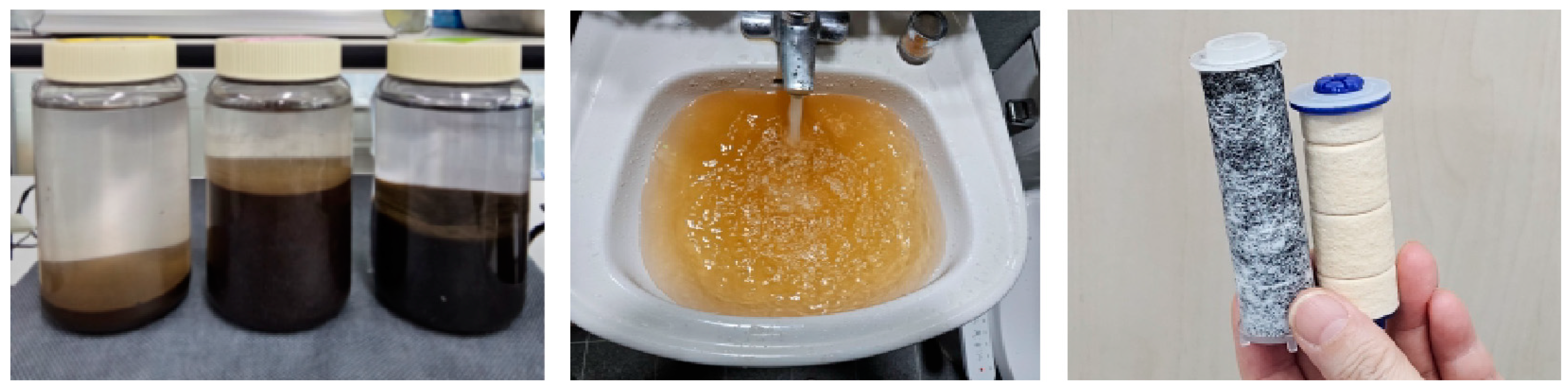
13]. Therefore, as depicted in
Figure 1, the results of water quality analysis performed using available turbidity and color tests do not accurately reflect the color of discolored tap water, thus, causing customer dissatisfaction.
To effectively respond to water quality issues caused by colored particles in tap water and address the limitations of water quality standard parameters such as turbidity and color, the National Institute of Environmental Research has proposed a filter test method for water quality management [
14]. However, this method involves visual inspection of filters’ color, making quantitative measurement difficult. Colorimeters and spectrophotometers have been extensively used in the food industry for color measurement [
15]. Therefore, in this study, we investigated a new test method by applying spectrophotometric colorimetry quantification.
2. Materials and Methods
2.1. Pipeline Status of the Study Area and Field Sample Collection
As of the end of 2021, Cheong-Ju (CJ) City, the study area in Chungcheongbuk-do, had a population of 836,711 individuals receiving water supply at a rate of 97.2%. The city supplies a total quantity of 350,000 m
3/d of domestic water from Jibuk (BJ) and CJ water treatment plants. The total length of pipelines in CJ City is 3066 km, and as shown in
Figure 2, 78% of them are ˂30 years old. Therefore, the proportion of aged pipes is relatively low.
Samples of sediments and coloring materials were obtained from pipes of a reservoir, a water tank, and an apartment during the supply of tap water in areas serviced by two water treatment plants located in CJ City (
Figure 3). The samples were collected at three points: The YulRang reservoir in Cheongwon-gu (Sample 1, YR), a Gagyeong Daewon apartment water tank in Heungdeok-gu (Sample 2, DT), and a Sachang Buheung apartment in Seowon-gu (Sample 3, BC). The pipe material, pipe diameter, and installation year at each sample collection point are presented in
Table 1.
2.2. Coloring Reference Material
The most common forms of Fe and Mn compounds, Fe
2O
3·H
2O and MnO
2, which cause discoloration of water in the DWDS, were selected as coloring reference materials and prepared as shown in
Table 2. The dissolved solution of iron (yellow) was prepared with a concentration of 1000 mg/L as Fe, using 1.62 g of 98% Fe
2O
3·H
2O. Similarly, the dissolved solution of manganese (black) was prepared at a concentration of 1000 mg/L as Mn, using 1.75 g of 90% MnO
2.
2.3. Analytical Equipment
2.3.1. Field Emission Scanning Electron Microscopy
In field emission scanning electron microscopy (FE–SEM), electrostatic and magnetic fields are combined to maximize the optical performance of the objective lens, thereby enabling excellent imaging of samples, including samples with characteristics similar to those of magnetic materials. Moreover, through the beam booster method, FE–SEM can capture images of particles less than a nanometer without an immersion lens at very low voltages (<1 kV).
The FE–SEM system used in this study was ULTRA Plus (ZEISS, Oberkochen, Germany) and the detector (energy dispersive X-ray spectroscopy, EDS) was XTrace (BRUKER, Berlin, Germany).
2.3.2. Inductively Coupled Plasma Optical Emission Spectroscopy
Inductively coupled plasma optical emission spectroscopy (ICP–OES) enables qualitative or quantitative analysis based on the wavelength and intensity of elements emitted by high-temperature plasma. Liquid samples are aerosolized and injected into high-temperature plasma for decomposition into atoms; the device then analyzes the atoms through ionization and excitation. The ICP–OES device used in this study was ARCOS FMX-36 (SPECTRO, Klev, Germany). For sample preprocessing, combining a microwave heating equipment with a high-pressure reactor enhances sample decomposition and shortens the processing time. The microwave equipment used in this study was UltraWAVE (Milestone, Sorisole, Italy).
2.3.3. Colorimetry
In the Drinking Water Quality Process Test Standard of South Korea, color measurement methods include visual colorimetric and spectrophotometric color measurement methods. Among the spectrophotometric methods, the multi-wavelength method (based on the principle of absorption) uses either the 10- or 30-division method. The wavelengths selected correspond to various organic and inorganic compounds that cause water coloration.
According to the Drinking Water Quality Process Test Standard, if a sample is turbid, color measurement using the multi-wavelength method is performed by determining the true color unit (TCU) after passing the sample through a 0.45 μm filter to eliminate any interference effects. Color measurement in this study was conducted using RICO 690 (HACH LANGE, Berlin, Germany).
2.3.4. Turbidity Measurement
Turbidity is measured based on the optical properties of water, where light is scattered and absorbed by particles. In South Korea, the turbidity of tap water is measured using the nephelometric turbidity unit (NTU) per the Drinking Water Quality Process Test Standard. The turbidity meter, equipped with a light source and photoelectric detector, uses a tungsten filament as the light source and detects scattered light. The color of the medium or measuring cell influences the turbidity measurement [
16]. In this study, we used HACH 2100AN (HACH Company, Loveland, CO, USA), which meets the criteria set in the Drinking Water Quality Process Test Standard, as the turbidity meter.
2.3.5. Spectrocolorimetry
Spectrocolorimeter (or spectrophotometer) and chroma meter are used to quantify color by assigning values to hue, brightness, and saturation, enabling the distinction of minute color differences not discernible by the human eye [
17].
There are color spaces or ways to represent the color, such as hue, value, saturation (HSV); red, green, blue (RGB); cyan, magenta, yellow, key (CMYK); and the data-based Commission Internationale de l’éclairage (CIE)/color space [
18]. In a 3D space, the distance between coordinates denotes color difference (
Figure 4) [
19].
In this study, we used a spectrocolorimeter equipped with a chroma meter (CM-700d model; KONICA MINOLTA, Tokyo, Japan,
Figure 4b).
2.4. Experimental
2.4.1. Experimental Method
To quantify coloring substances in tap water, we aimed to develop a new membrane filter colorimetry (MFC) method that quantifies the color difference, △E*ab. We performed color cross-testing and measured turbidity to confirm the limitations of available methods. Furthermore, we quantified coloring substances such as Fe and Mn compounds in the samples using scanning electron microscopy/energy-dispersive X-ray spectroscopy (SEM–EDS) and ICP–OES, prepared standard solutions of similar concentrations, and passed the samples and standard solutions through a 0.45 μm filter. The samples and standard solutions were analyzed using a spectrocolorimeter.
2.4.2. Review of Previous Testing Methods
In this study, we considered two methods. The first method was the filter test method (FTM), in which color is measured visually by passing a solution through a filter and then observing the color of the filter paper, per the guidelines for the use of FTM by the National Institute of Environmental Research (NIER). The second was the membrane patch colorimetry (MPC) method, in which color is quantified spectroscopically by first filtering lubricant oil and measuring the color of the filter paper using a colorimeter, per the “Standard Test Method for Measurement of Lubricant Generated Insoluble Color Bodies in In-Service Turbine Oils using Membrane Patch Colorimetry” by the American Society for Testing and Materials (ASTM).
The approaches currently used by the NIER and ASTM measure colorants in drinking water and lubricant oil; they have advantages and disadvantages in terms of specificity of samples and quantification methods. Therefore, we combined the beneficial elements of these two methods and modified them to develop a new test method, MFC.
Table 3 presents a comparison of the new and old test methods.
2.4.3. Application of MFC
MFC, developed by combining and modifying the FTM of NIER-GP2020-177 (2021) and MPC of ASTM D7843-21 (2023), was used to quantitatively measure colorants that occur during the supply of tap water. The MPC test results are expressed as filter color units (FCU).
This testing method can be used to analyze insoluble coloring substances in drinking water (e.g., tap water) by using a filter according to the standards in
Table 4, following the procedure described below.
The procedure of MFC is as follows.
A filter was positioned between the filter support and funnel and secured using a filter holder. The filter was then moistened using a small amount of water, and a vacuum (33 kPa↓) was applied. The sample was then vigorously mixed for 30 s to homogenize the coloring substance. Immediately after mixing, 1 L of the sample was poured into the filter funnel, which was then rinsed with at least 35 mL of water to allow the filtrate to flow completely. Subsequently, the vacuum was turned off; the filter was separated, placed in a Petri dish, and allowed to air-dry for 3 h. Thereafter, the background color was measured using a spectrocolorimeter with the same filter used to filter the 1 L of distilled water. The color difference (ΔE*ab) between the measured distilled water background color and the sample was selected, and the CIELAB ΔE*ab value of the spectrocolorimeter to the first decimal place was recorded. The ΔE value is expressed as FCU. If the ΔE*ab value was 4.0, it was read as 4.0 FCUs.
3. Results and Discussion
3.1. Elemental Analysis of Samples
To identify the elements of colorants that leak from water storage tank sediments and pipe networks, we analyzed the samples using FESEM–EDS and ICP–OES.
The results of the FESEM–EDS analysis revealed that the concentrations of oxygen (O, 56.4%) and carbon (C, 29.4%) were the highest, followed by those of nitrogen (N, 7.9%), aluminum (Al, 1.6%), Fe (3.5%), Mn (0.25%), silicon (Si, 0.34%), zinc (Zn, 0.45%), and chlorine (Cl, 0.09%). Furthermore, the analysis revealed that Al residues from coagulants used in water treatment and organic compounds C, O, and N in their oxidized forms, which were either not fully treated during the water treatment process or resuspended within the pipe network, were the elements present at the highest concentrations. In addition, it was determined that the water could become discolored when substances containing coloring inorganic elements such as Fe and Mn were ejected.
Figure 5 presents the analysis results of sediments obtained from the water supply system in CJ City to further accurately compare the SEM–EDS analysis results.
Furthermore, the ICP–OES analysis of the samples obtained from the CJ City water supply system revealed that the concentration of colorants in samples increased from an average of 165.14 to 235.53 mg/kg for Fe and decreased from 113.81 to 6.00 mg/kg for Mn in the YR, DT, and BC samples (
Table 5 and
Figure 6). These results are consistent with the FESEM–EDS analysis results, in which, the Fe concentration increased to 1.16%, 1.31%, and 8.12% in the YR, DT, and BC samples, respectively, and the Mn concentration decreased to 0.60%, 0.14%, and 0%, respectively. It is evident that in the water distribution network, the concentration of Mn not treated in the water treatment process decreases, as Mn settles in reservoirs and tanks, whereas that of Fe increases due to pipe corrosion. Based on FESEM–EDS test results, reference materials were prepared according to the content of Fe and Mn.
3.2. Color and Turbidity Cross-Test
A cross-test of color and turbidity was conducted to determine the limitations of available color and turbidity test methods. The turbidity was measured using a color standard solution of potassium hexachloroplatinate and cobalt chloride (K
2PtCl
6+CoCl
2⋅6H
2O), according to the standard methods. The color was measured using a turbidity standard solution of hydrazine sulphate and hexamethylenetetramine ((NH
2)
2⋅H
2SO
4+(CH
2)
6N
4). The results are shown in
Table 6.
Based on the cross-test results (
Table 6), the turbidity of the color standard solution (1–50 color units (CU)) was consistently within the range of 0.052–0.081 NTU, regardless of the concentration of the solution, demonstrating the difficulty in measuring the color standard solution with turbidity. These results are consistent with those of II-Seon et al. [
19], suggesting that the scattering of light differs depending on the wavelength when using broad-spectrum (white) light, which causes the medium to act as a filter and the color of the medium or measuring cell to influence turbidity. Our findings indicate the limitations of the available turbidity test methods and possibly explain why the turbidity quality standard appears to be suitable even when household filters become discolored during tap water discoloration events.
However, the color of the turbidity standard solution without filtration was 0.4 CU at 0.1 NTU and displayed an increasing trend at an average of 1.4, 2.0, 5.0, 14.6, and 25.0 CU according to 0.3, 0.5, 1.0, 3.0, and 5.0 NTU, respectively. However, when the turbid matter was removed using a filter, the TCU of all samples was 0. This result suggests that there are limitations in the quality testing of tap water during typical discoloration events, which involve turbidity and color.
3.3. MFC Test of Field Samples
To establish an effective method to test discoloration of field samples collected from the DWDS, three samples collected from a reservoir, a tank, and an apartment were subjected to conventional turbidity and color tests and MFC.
We diluted each of the three samples at 1/20,000 dilution based on 0.5NTU. The average turbidity values of the diluted samples are shown in
Table 7; they appeared to decrease in the following order: YR > DT > BC. This result can be attributed to both the turbidity and color of the samples contributing to the turbidity. Moreover, all color measurements, recorded as TCU after removing turbidity, were 0, indicating that the available color testing method is not feasible for colored samples.
As shown in
Figure 7 and
Figure 8, the ΔE*ab values (D65) of YR, DT, and BC samples increased proportionally with their concentrations. As shown in
Table 8, the R
2 values were 0.8971, 0.9788, and 0.9881 for YR, DT, and BC samples, respectively, indicating that the color difference can be used to quantitatively measure coloring substances.
3.4. MFC Test Results of the Coloring Reference Material
To verify the colorimetry results for Fe and Mn, we prepared reference materials using Fe
2O
3·H
2O (yellow iron oxide) and MnO
2 (manganese dioxide); the concentrations of Fe and Mn corresponded to those in the field samples.
Table 9 presents the calculated values of the Fe and Mn concentrations for the same field sample, as outlined in
Table 7. These calculations were performed to determine the range of iron and manganese addition amounts for the subsequent experiment. Through this analysis, we confirmed that the average concentrations of Fe and Mn ranged from 1.7 to 235.5 μg/kg and 0.06 to 113.8 μg/kg, respectively. Based on the Fe concentration, we then prepared the reference materials of Fe and Mn ranging from 1 to 500 μg/L (
Table 10).
The experimental results of the reference materials, shown in
Table 11, indicate a proportional increase in turbidity with the increase in sample concentration. However, the intensity of color increased almost proportionally depending on the sample before filtration with a 0.45 μm filter; however, after filtration according to the Drinking Water Quality Process Test Standard, all color values were 0.
The coloring reference material solutions were passed through filters, which were then dried at room temperature for 3 h. We conducted an MFC test of the discolored surface of the dried filter. As shown in
Figure 9 and
Figure 10, the color difference ΔE*ab (D65) increased with the concentration of the Fe and Mn reference materials in the YR, DT, and BC samples. The regression analysis between the reference material concentration and color difference (
Table 12) revealed a high concentration of the Fe and Mn reference materials in the YR, DT, and BC samples. The regression analysis between the reference materials and MnO
2 might be a useful method for measuring colorants within the range of the Fe and Mn content and ratio in field samples.
A comparison of the FCU values of the CIE reference material and the coloring reference material (
Table 13 and
Figure 11) showed that the FCU values of the field samples, based on Fe, were higher than those of the reference materials. This finding suggests that the field samples contain not only colorants such as Fe and Mn but also other substances causing coloration, which might have increased the FCU values. The FCU values of the field samples decreased in the following order: YR > DT > BC, with sediment showing a higher FCU than rust water in the water supply system. The high determination coefficients between the FCU of the field samples (YR, DT, and BC) and that of the coloring reference material suggest that measuring FCU using MFC could be a useful method in cases of tap water discoloration events.
4. Conclusions
In this study, we analyzed coloring materials in the tap water supply of CJ City and Fe and Mn reference materials using a spectrocolorimeter and other instruments to develop an effective method for determining discoloration events in the DWDS. Analysis using FESEM–EDS and ICP–OES identified O (56.4%), C (29.4%), and Al (1.6%), in addition to Fe (3.5%) and Mn (0.25%), which are known colorants in tap water. In YR, DT, and BC, the average concentration of Fe increased from 165.14 to 235.53 mg/kg, whereas that of Mn decreased from 113.81 to 6.00 mg/kg.
Furthermore, the cross-test results between color and turbidity showed that color standard solutions from 1 to 50 CU closely corresponded with turbidity values from 0.052 to 0.081 NTU. In addition, the turbidity values of the standard solutions from 0.1 to 5.0 NTU corresponded to color values from 0.4 to 25.0 CU. However, when turbid matter was removed using a 0.45 μm filter, according to the Drinking Water Quality Process Test Standard, TCU was zero in all samples. This finding demonstrates the limitations of measuring coloring substances in tap water using available test methods for turbidity and color.
We conducted MFC on stepwise diluted YR, DT, and BC field samples and measured the filter color (FCU = ΔE*ab (D65)). The FCU R2 values of the samples were 0.8971, 0.9788, and 0.9881, respectively, according to the sample volume. Moreover, the regression analysis of FCU of the coloring reference materials prepared using Fe and Mn at concentrations observed in the field samples yielded high R2 values of 0.9662, 0.9803, and 0.9726, respectively.
The high determination coefficients (R2 = 0.9770, 0.9927, and 0.9954, respectively) between the FCU of the field samples (YR, DT, and BC) and that of the coloring reference material suggest that the use of ΔE*ab measured using MFC could be an effective method to quantitatively analyze discolored tap water. Therefore, we propose adopting FCU as a new water quality standard by accumulating and analyzing inspection results based on MPC in future research.
Author Contributions
Conceptualization: D.-H.K.; Data Curation: D.-H.K. and H.-B.J.; Formal Analysis: D.-H.K., J.-G.L., J.-H.K. and S.-W.K.; Funding Acquisition: D.-H.K. and H.-B.J.; Investigation: D.-H.K. and J.-H.K.; Methodology: D.-H.K. and J.-G.L.; Project Administration: H.-B.J.; Resources: D.-H.K., J.-G.L. and H.-B.J.; Software: J.-H.K. and S.-W.K.; Supervision: H.-B.J.; Validation: D.-H.K.; Visualization: D.-H.K.; Writing—original draft: D.-H.K. and J.-G.L.; Writing—review and editing: J.-H.K., S.-W.K. and H.-B.J. All authors have read and agreed to the published version of the manuscript.
Funding
This work is financially supported by Korea Ministry of Environment (MOE) as Waste to Energy-Recycling Human Resource Development Project.
Data Availability Statement
The data presented in this study are available on request from the corresponding author.
Conflicts of Interest
Authors Kwon Jin-Hong and Kim Sang-Woo were employed by the company Korea Environmental Industry & Technology Institute Co., Ltd. The remaining authors declare that the research was conducted in the absence of any commercial or financial relationships that could be construed as a potential conflict of interest.
References
- Vreeburg, J.H.G. Discolouration in Drinking Watersystems, The Role of Particles Clarified, KWA Water Cycle Research Institute Series; IWA Publishing: Washington, DC, USA, 2010. [Google Scholar]
- Vreeburg, J.H.G.; Schippers, D.; Verberk, J.Q.J.C.; van Dijk, J.C. Impact of particles on sediment accumulation in a drinking water distribution system. Water Res. 2008, 42, 4233–4242. [Google Scholar] [CrossRef] [PubMed]
- Boxall, J.B.; Skipworth, P.J.; Saul, A.J. Aggressive flushing for discolouration event mitigation in water distribution networks. Water Sci. Technol. Water Supply 2003, 3, 179–186. [Google Scholar] [CrossRef]
- Slaats, P.G.G.; Rosenthal, L.P.M.; Sieger, W.G.; van den Boomen, M.; Beuken, R.H.S.; Vreeburg, J.H.G. Processes Involved in Generation of Discoloured Water; Report No. KOA 02; Awwa Research Foundation: Denver, CO, USA, 2002; Volume 058. [Google Scholar]
- Weber, W.J.; Smith, E.H. Simulation and design models for adsorption processes. Environ. Sci. Technol. 1987, 21, 1040–1050. [Google Scholar] [CrossRef]
- Kawamura, S. Integrated Design of Water Treatment Facilities; John Willey & Sons, Inc.: Washington, DC, USA, 1997; pp. 539–545. [Google Scholar]
- Johnson, C.A.; Ulrich, M.; Sigg, L.; Imboden, D.M. A mathematical model of the manganese cycle in a seasonally anoxic lake. Limnol. Oceanogr. 1991, 36, 1415–1426. [Google Scholar] [CrossRef]
- Sommerfeld, E.O. Iron and Manganese Removal Handbook; American Water Works Association: Denver, CO, USA, 1999. [Google Scholar]
- AWWA. Water Quality and Treatment, 5th ed.; American Water Works Association: Denver, CO, USA, 1999. [Google Scholar]
- Vreeburg, J.H.G.; Boxall, J.B. Discolouration in potable water distribution systems: A review. Water Res. 2007, 41, 519–529. [Google Scholar] [CrossRef] [PubMed]
- National Institute of Environmental Research. Guidelines for Utilizing Filter Test Methods; NIER: Incheon, Republic of Korea, 2020.
- Ministry of the Environment. Tap Water Drinking Survey; MOE: Sejong, Republic of Korea, 2021; Volume 2021.
- Ministry of the Environment. Rules on Drinking Water Quality Standards and Inspection; MOE: Sejong, Republic of Koreas, 2021.
- Ministry of the Environment. Water Resources Management Information System. Available online: https://www.nier.go.kr/NIER/cop/bbs/selectNoLoginBoardArticle.do?menuNo=14003&bbsId=BBSMSTR_000000000022&nttId=27827&Command=READ (accessed on 15 September 2023).
- Balaban, M.O.; Odabasi, A.Z. Measuring Color with Machine Vision. Food Technol. 2006, 60, 32–36. [Google Scholar]
- Park, J.W.; Byun, K.; Cho, S.Y.; Kim, B.S.; Oh, J.H. A Study on Rapid Color Difference Discrimination for Fabrics using Digital Imaging Device. J. Korea Acad.-Ind. Coop. Soc. 2019, 20, 29–37. [Google Scholar]
- Serup, J.; Agner, T. Colorimetric quantification of erythemaaA comparison of two colorimeters (Lange Micro Color and Minolta Chroma Meter CR200) with a clinical scoring scheme and laser Doppler flowmetry. Clin. Exp. Dermatol. 1990, 15, 267–272. [Google Scholar] [CrossRef]
- Smith, A.R. Color gamut transform pairs. SIGGRAPH Comput. Graph. 1978, 12, 12–19. [Google Scholar] [CrossRef]
- Belasco, R.; Edwards, T.; Munoz, A.J.; Rayo, V.; Buono, M.J. The effect of hydration on urine color objectively evaluated in CIE L*a*b* color space. Front. Nutr. 2020, 7, 576974. [Google Scholar] [CrossRef]
Figure 1.
Images of discolored water and filters before and after use (left: turbidity-causing deposits; middle: discolored tap water; right: colored particles in tap water).
Figure 1.
Images of discolored water and filters before and after use (left: turbidity-causing deposits; middle: discolored tap water; right: colored particles in tap water).
Figure 2.
Current status of water supply pipe burial period in CJ city.
Figure 2.
Current status of water supply pipe burial period in CJ city.
Figure 3.
Field sample collection area (Google map).
Figure 3.
Field sample collection area (Google map).
Figure 4.
CIE L*a*b* color space (a). Portable spectrocolorimeter CM-700d (b). L represents brightness between 100 (white) and 0 (black), whereas a and b represent color (–a, green; +a, red; −b, blue; +b, yellow).
Figure 4.
CIE L*a*b* color space (a). Portable spectrocolorimeter CM-700d (b). L represents brightness between 100 (white) and 0 (black), whereas a and b represent color (–a, green; +a, red; −b, blue; +b, yellow).
Figure 5.
Percentage weight of main elements determined using SEM–EDS analysis.
Figure 5.
Percentage weight of main elements determined using SEM–EDS analysis.
Figure 6.
Changes in the iron and manganese concentrations of samples.
Figure 6.
Changes in the iron and manganese concentrations of samples.
Figure 7.
Filter photographs of the field samples.
Figure 7.
Filter photographs of the field samples.
Figure 8.
ΔE*ab (d65) of the field samples.
Figure 8.
ΔE*ab (d65) of the field samples.
Figure 9.
Filter photographs of the reference material.
Figure 9.
Filter photographs of the reference material.
Figure 10.
FCU of the reference material.
Figure 10.
FCU of the reference material.
Figure 11.
FCU (ΔE*ab) of the sample and reference materials YR (a), DT (b), BC (c).
Figure 11.
FCU (ΔE*ab) of the sample and reference materials YR (a), DT (b), BC (c).
Table 1.
Characteristics of inflow pipes by sampling points.
Table 1.
Characteristics of inflow pipes by sampling points.
| Sample | Classification | Pipe Material (s) | Pipe Size | Laying Year |
|---|
| Sa1. YR | Service reservoir | PE-3 | 700 mm | 2014 |
| Sa2. DT | Water storage tank | Ductile cast iron pipe | 100 mm | 1998 |
| Sa3. BC | Consumer supply pipe | Steel/polyvinyl chloride | 15 mm | 1984 |
Table 2.
Specifications of the reference materials.
Table 2.
Specifications of the reference materials.
| Chemical Formula | Fe2O3·H2O | MnO2 |
|---|
| Chemical Name | Yellow iron oxide | Manganese dioxide |
| CAS No. | 51274-00-1 | 1313-13-9 |
| Manufacturer | JUNSEI, Tokyo, Japan (32226-1601) | JUNSEI, Tokyo, Japan (53165-0401) |
Dissolved solution color
(1000 mg/L) | ![Water 15 04137 i001]() | ![Water 15 04137 i002]() |
Table 3.
Development of MFC using FTM and MPC.
Table 3.
Development of MFC using FTM and MPC.
| Division | Application | Quantification Method | Method |
|---|
| Lubricant | Water | Spectrometry | Eyesight |
|---|
| (1) NIER | | ● | | ● | FTM |
| (2) ASTM | ● | | ● | | MPC |
| (3) This Study | | ● | ● | | MFC |
![Water 15 04137 i003]() |
Table 4.
Overview of the membrane filter colorimetry test method.
Table 4.
Overview of the membrane filter colorimetry test method.
| Parameter | Filtration Volume | Filter and
Pore Size | Material | Vacuum |
|---|
| Criteria | 1 L | 47 mm, 0.45 μm | Membrane * | 33 kPa↓ |
Table 5.
Concentration of iron and manganese in field samples.
Table 5.
Concentration of iron and manganese in field samples.
| Sample | Element | Mean
(mg/kg) | Max
(mg/kg) | Min
(mg/kg) | Standard Deviation
(S) |
|---|
YR
Reservoir | Fe | 165.14 | 166.8 | 164.2 | 1.2 |
| Mn | 113.81 | 118.4 | 111.2 | 3.3 |
DT
Water tank | Fe | 184.61 | 186.5 | 183.2 | 1.4 |
| Mn | 20.02 | 20.3 | 19.8 | 0.2 |
BC
apartment | Fe | 235.53 | 244.1 | 221.5 | 10.0 |
| Mn | 6.00 | 6.1 | 5.9 | 0.1 |
Table 6.
Cross-test of turbidity and color.
Table 6.
Cross-test of turbidity and color.
| Color | Turbidity | Turbidity | Color |
|---|
Std
(CU) 1 | Avg
(CU) | min
(NTU) 2 | max
(NTU) | Std
(NTU) | Avg
(NTU) | Direct
(CU) | Filter
(TCU) 3 |
|---|
| 1 | 1.0 ± 0.00 | 0.055 | 0.070 | 0.1 | 0.13 ± 0.01 | 0.4 ± 0.49 | 0 |
| 3 | 3.0 ± 0.00 | 0.052 | 0.075 | 0.3 | 0.31 ± 0.02 | 1.4 ± 0.49 | 0 |
| 5 | 5.0 ± 0.00 | 0.054 | 0.065 | 0.5 | 0.51 ± 0.01 | 2.0 ± 0.00 | 0 |
| 10 | 10.2 ± 0.40 | 0.055 | 0.079 | 1.0 | 1.02 ± 0.04 | 5.0 ± 0.00 | 0 |
| 30 | 31.0 ± 0.00 | 0.050 | 0.081 | 3.0 | 2.85 ± 0.18 | 14.6 ± 0.49 | 0 |
| 50 | 52.4 ± 0.49 | 0.057 | 0.075 | 5.0 | 4.77 ± 0.28 | 25.0 ± 0.89 | 0 |
Table 7.
Average of turbidity and color values of the field samples.
Table 7.
Average of turbidity and color values of the field samples.
| Sample (μL/L) | 10 | 30 | 50 | 100 | 300 | 500 | 1000 |
|---|
T
U
R
B | NTU | YR | 0.14 | 0.33 | 0.51 | 1.02 | 2.92 | 4.98 | 9.95 |
| DT | 0.12 | 0.28 | 0.45 | 0.82 | 2.03 | 3.39 | 6.54 |
| BC | 0.16 | 0.32 | 0.52 | 0.98 | 2.76 | 4.54 | 8.82 |
C
O
L
O
R | CU | YR | 0.00 | 1.00 | 1.00 | 2.00 | 6.20 | 11.00 | 21.00 |
| DT | 0.00 | 0.00 | 0.40 | 0.80 | 2.20 | 4.00 | 7.60 |
| BC | 0.00 | 0.00 | 0.00 | 0.60 | 1.00 | 2.20 | 4.40 |
| TCU | YR | 0 | 0 | 0 | 0 | 0 | 0 | 0 |
| DT | 0 | 0 | 0 | 0 | 0 | 0 | 0 |
| BC | 0 | 0 | 0 | 0 | 0 | 0 | 0 |
Table 8.
Mean ΔE*ab (D65) of the field samples.
Table 8.
Mean ΔE*ab (D65) of the field samples.
Sample
Concentration
(μL/L) | ΔE*ab (D65) |
|---|
| Sa1. YR | Sa2. DT | Sa3. BC |
|---|
| Mean ± SD | Min–Max | Mean ± SD | Min–Max | Mean ± SD | Min–Max |
|---|
| 10 | 2.22 ± 0.23 | 1.80–2.44 | 1.01 ± 0.09 | 0.88–1.14 | 1.21 ± 0.17 | 0.94–1.43 |
| 30 | 6.67 ± 0.29 | 6.41–7.24 | 2.86 ± 0.16 | 2.60–3.07 | 3.63 ± 0.30 | 3.07–3.92 |
| 50 | 10.85 ± 0.45 | 10.48–11.63 | 4.83 ± 0.28 | 4.34–5.20 | 5.40 ± 0.37 | 4.70–5.70 |
| 100 | 21.39 ± 2,23 | 19.83–25.82 | 9.31 ± 0.29 | 8.78–9.56 | 10.76 ± 0.82 | 9.50–11.88 |
| 300 | 44.57 ± 0.37 | 44.17–45.23 | 25.40 ± 0.36 | 24.87–25.83 | 24.87 ± 0.64 | 24.00–25.63 |
| 500 | 54.10 ± 0.22 | 53.88–54.38 | 37.60 ± 0.66 | 36.28–38.07 | 38.37 ± 0.72 | 37.45–39.65 |
| 1000 | 60.50 ± 0.56 | 59.44–61.47 | 54.39 ± 0.19 | 54.08–54.67 | 59.21 ± 1.52 | 56.73–61.41 |
| R2 | 0.8971 | 0.9788 | 0.9881 |
Table 9.
Content of iron and manganese in diluted field samples.
Table 9.
Content of iron and manganese in diluted field samples.
| Sample | Concentration
(μg/L) | 10 | 30 | 50 | 100 | 300 | 500 | 1000 |
|---|
| YR | Fe | 1.7 | 5.0 | 8.3 | 16.5 | 49.5 | 82.6 | 165.1 |
| Mn | 1.1 | 3.4 | 5.7 | 11.4 | 34.1 | 56.9 | 113.8 |
| DT | F | 1.8 | 5.5 | 9.2 | 18.5 | 55.3 | 92.3 | 184.6 |
| Mn | 0.2 | 0.6 | 1.0 | 2.0 | 6.0 | 10.0 | 20.0 |
| BC | Fe | 2.4 | 7.1 | 11.8 | 23.6 | 70.1 | 117.8 | 235.5 |
| Mn | 0.06 | 0.18 | 0.30 | 0.60 | 1.8 | 3.00 | 6.00 |
Table 10.
Concentration of iron and manganese in samples used in the MFC test.
Table 10.
Concentration of iron and manganese in samples used in the MFC test.
| Sample | Element | Concentration (μg/L) |
|---|
| YR | Fe | 1 | 5 | 10 | 30 | 50 | 100 | 200 | 300 | 500 |
| Mn | 0.689 | 3.45 | 6.89 | 20.68 | 34.46 | 68.92 | 137.8 | 206.8 | 344.6 |
| DT | Fe | 1 | 5 | 10 | 30 | 50 | 100 | 200 | 300 | 500 |
| Mn | 0.108 | 0.542 | 1.08 | 3.25 | 5.42 | 10.84 | 21.68 | 32.52 | 54.20 |
| BC | Fe | 1 | 5 | 10 | 30 | 50 | 100 | 200 | 300 | 500 |
| Mn | 0.026 | 0.128 | 0.26 | 0.77 | 1.28 | 2.55 | 5.10 | 7.65 | 12.75 |
Table 11.
Turbidity (NTU) and chromaticity (CU, TCU) of the reference material.
Table 11.
Turbidity (NTU) and chromaticity (CU, TCU) of the reference material.
| RM | 1 | 5 | 10 | 30 | 50 | 100 | 200 | 300 | 500 |
|---|
| NTU | YR | 0.10 | 0.19 | 0.29 | 0.76 | 1.16 | 2.28 | 4.44 | 6.63 | 10.92 |
| DT | 0.10 | 0.18 | 0.28 | 0.71 | 1.10 | 2.09 | 4.16 | 6.13 | 10.18 |
| BC | 0.10 | 0.18 | 0.26 | 0.66 | 1.10 | 2.08 | 4.14 | 9.84 | 9.96 |
| CU | YR | 0.0 | 0.0 | 0.0 | 1.0 | 1.0 | 1.8 | 3.0 | 4.8 | 7.2 |
| DT | 0.0 | 0.0 | 0.0 | 0.6 | 1.0 | 1.6 | 2.6 | 3.8 | 6.0 |
| BC | 0.0 | 0.0 | 0.0 | 0.8 | 1.0 | 1.2 | 2.0 | 3.0 | 5.0 |
| TCU | YR | 0 | 0 | 0 | 0 | 0 | 0 | 0 | 0 | 0 |
| DT | 0 | 0 | 0 | 0 | 0 | 0 | 0 | 0 | 0 |
| BC | 0 | 0 | 0 | 0 | 0 | 0 | 0 | 0 | 0 |
Table 12.
Mean ΔE*ab values of the reference material.
Table 12.
Mean ΔE*ab values of the reference material.
RM
(µg/L) | ΔE*ab (D65) |
|---|
| Sa1. YR | Sa2. DT | Sa3. BC |
|---|
| Mean ± S.D | Min–Max | Mean ± S.D | Min–Max | Mean ± S.D | Min–Max |
|---|
| 1 | 0.47 ± 0.01 | 0.45–0.49 | 0.48 ± 0.04 | 0.42–0.53 | 0.60 ± 0.03 | 0.57–0.65 |
| 5 | 1.52 ± 0.04 | 1.45–1.58 | 1.39 ± 0.08 | 1.29–1.48 | 1.21 ± 0.09 | 1.09–1.32 |
| 10 | 2.90 ± 0.42 | 2.21–3.47 | 2.51 ± 0.21 | 2.16–2.78 | 2.14 ± 0.18 | 1.90–2.40 |
| 30 | 8.15 ± 0.47 | 7.41–8.74 | 7.59 ± 1.33 | 5.96–9.78 | 6.68 ± 0.47 | 6.13–7.35 |
| 50 | 12.64 ± 0.59 | 11.88–13.54 | 11.43 ± 0.82 | 9.92–12.38 | 10.99 ± 0.90 | 9.90–12.15 |
| 100 | 23.86 ± 0.69 | 22.85–24.62 | 20.92 ± 1.51 | 19.53–23.43 | 20.37 ± 0.81 | 19.37–21.22 |
| 200 | 39.20 ± 0.77 | 37.73–39.95 | 37.81 ± 2.08 | 34.51–40.74 | 37.47 ± 1.61 | 35.06–39.28 |
| 300 | 48.33 ± 1.67 | 45.59–50.11 | 48.57 ± 3.01 | 43.91~51.92 | 51.81 ± 6.56 | 47.61~64.87 |
| 500 | 58.76 ± 1.16 | 56.67–59.86 | 63.64 ± 2.47 | 60.55~66.06 | 61.59 ± 6.05 | 49.82~66.25 |
| R2 | 0.9662 | 0.9803 | 0.9726 |
Table 13.
Mean FCU values of field samples and reference material.
Table 13.
Mean FCU values of field samples and reference material.
| No. | YR | DT | BC |
|---|
| Sample | RM | Sample | RM | Sample | RM |
|---|
| Fe | FCU | Fe | FCU | Fe | FCU | Fe | FCU | Fe | FCU | Fe | FCU |
|---|
| 1 | 1.7 | 2.2 | 1 | 0.5 | 1.8 | 1.0 | 1 | 0.5 | 2.4 | 1.2 | 1 | 0.6 |
| 2 | 5.0 | 6.7 | 5 | 1.5 | 5.5 | 2.9 | 5 | 1.4 | 7.1 | 3.6 | 5 | 1.2 |
| 3 | 8.3 | 10.8 | 10 | 2.9 | 9.2 | 4.8 | 10 | 2.5 | 11.8 | 5.4 | 10 | 2.1 |
| 4 | 16.5 | 21.4 | 30 | 8.2 | 18.5 | 9.3 | 30 | 7.6 | 23.6 | 10.8 | 30 | 6.7 |
| 5 | 41.3 | 44.6 | 50 | 12.6 | 46.2 | 25.4 | 50 | 11.4 | 58.9 | 24.9 | 50 | 11.0 |
| 6 | 82.6 | 54.1 | 100 | 23.9 | 92.3 | 37.6 | 100 | 20.9 | 117.8 | 38.4 | 100 | 20.4 |
| 7 | 165.1 | 60.5 | 200 | 39.2 | 184.6 | 54.4 | 200 | 37.8 | 235.5 | 59.2 | 200 | 37.5 |
| 8 | | | 300 | 48.3 | | | 300 | 48.6 | | | 300 | 51.8 |
| 9 | | | 500 | 58.8 | | | 500 | 63.6 | | | 500 | 61.6 |
| R2 | 0.9770 | 0.9927 | 0.9954 |
| Disclaimer/Publisher’s Note: The statements, opinions and data contained in all publications are solely those of the individual author(s) and contributor(s) and not of MDPI and/or the editor(s). MDPI and/or the editor(s) disclaim responsibility for any injury to people or property resulting from any ideas, methods, instructions or products referred to in the content. |
© 2023 by the authors. Licensee MDPI, Basel, Switzerland. This article is an open access article distributed under the terms and conditions of the Creative Commons Attribution (CC BY) license (https://creativecommons.org/licenses/by/4.0/).


