
Organochlorine Pesticides in Soil–Groundwater–Plant System in a Famous Agricultural Production Area in China: Spatial Distribution, Source Identification and Migration Prediction

 ,
,
Abstract
:1. Introduction
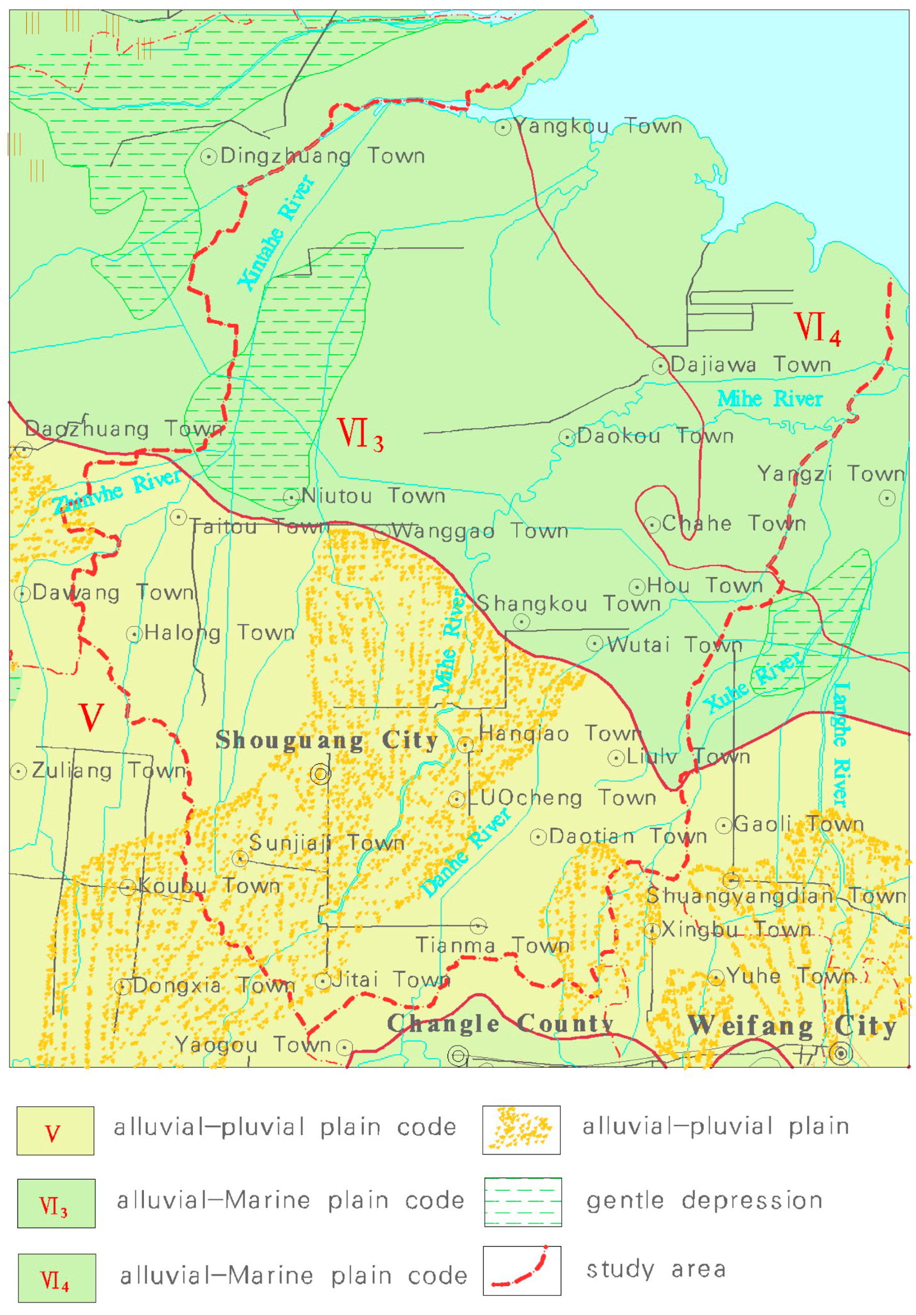
2. Study Area
3. Materials and Methods
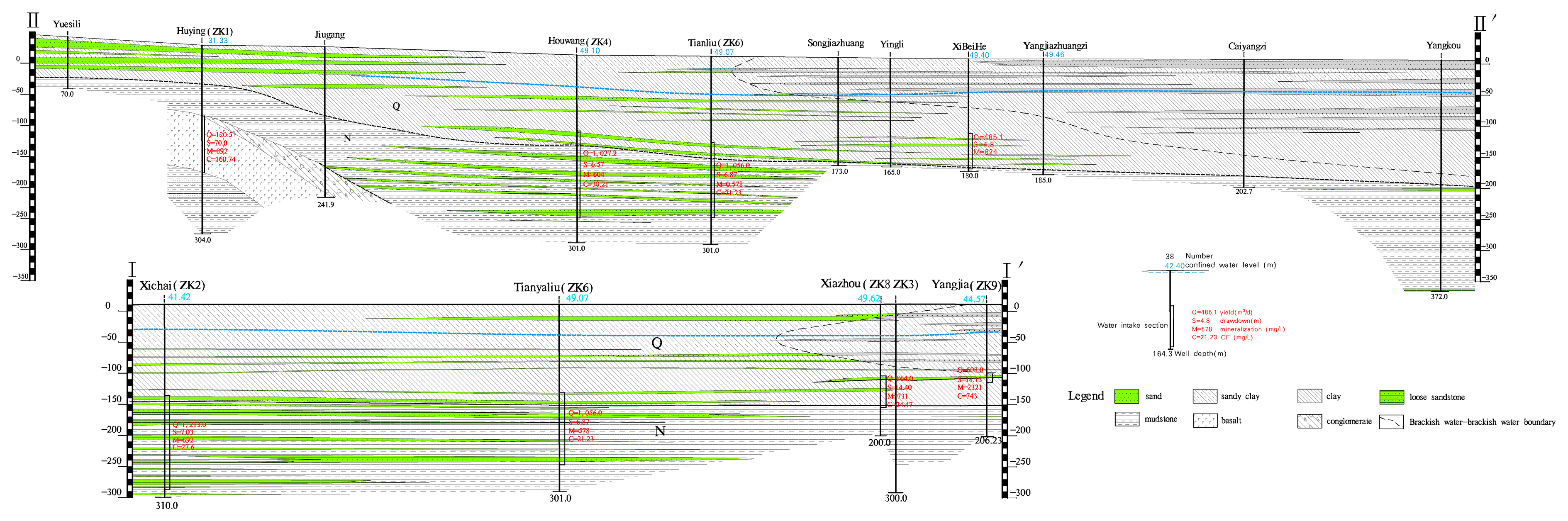
3.1. Groundwater Types and Water Abundance Characteristics
3.2. Recharge, Runoff and Discharge of Shallow Pore Water
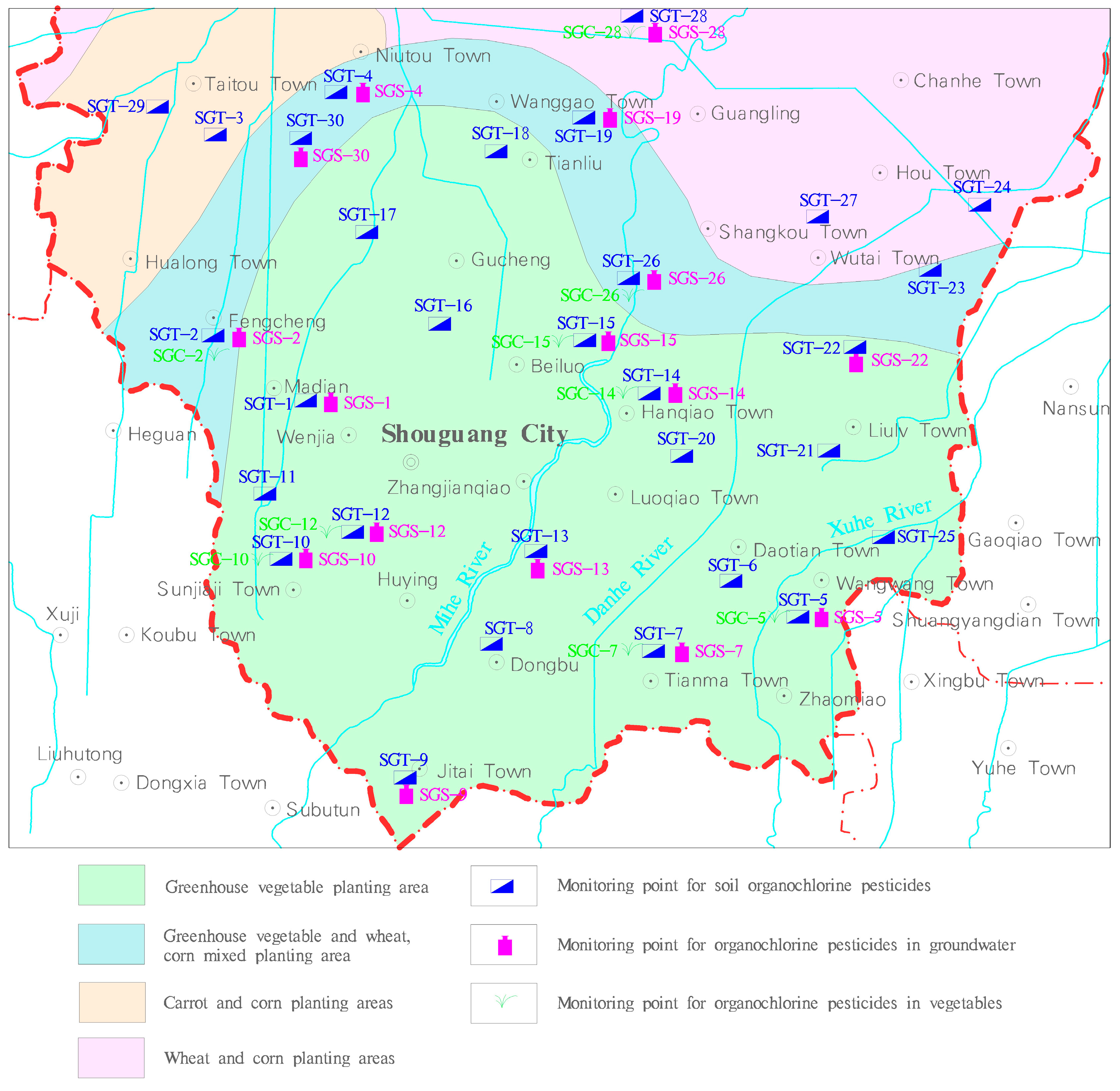
3.3. Vegetable Planting
3.4. General Situation of Pesticide Use
3.5. Sample Collection and Testing
3.5.1. Soil Sample
3.5.2. Water Sample
3.5.3. Plant Sample
3.5.4. Testing
3.6. Numerical Simulation
3.6.1. Model Area
3.6.2. Aquifer Generalization
3.6.3. Generalization of Boundary Conditions
3.6.4. Simulated Flow Field and Sources-Sinks
3.6.5. Hydrogeological Parameters
3.6.6. Numerical Model
3.7. Solute Transport Model
3.7.1. Simulation Principle
3.7.2. Groundwater Flow Field
3.7.3. Simulation Parameters
3.7.4. Simulated Source Strength
3.8. Model Identification, Verification and Prediction
4. Results and Discussion
4.1. Distribution of OCPs in Soil
4.1.1. Detection and Content of Topsoil
4.1.2. Changing Trend of OCPs in Topsoil
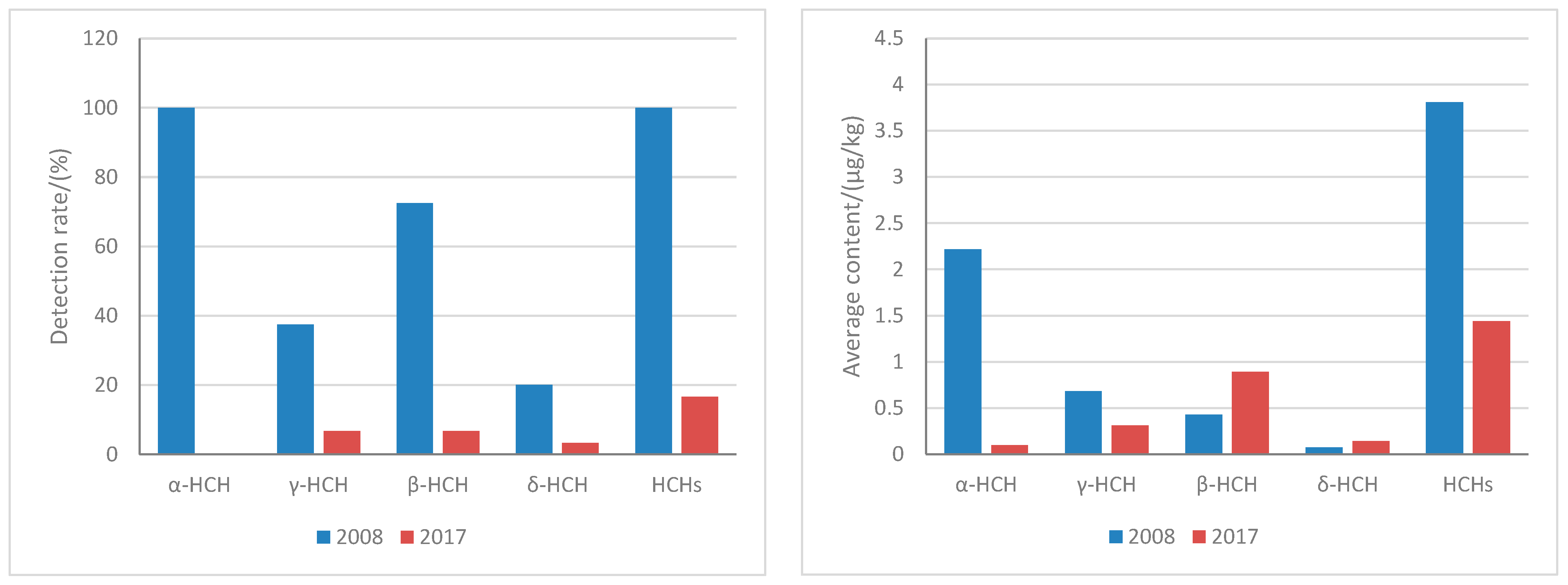
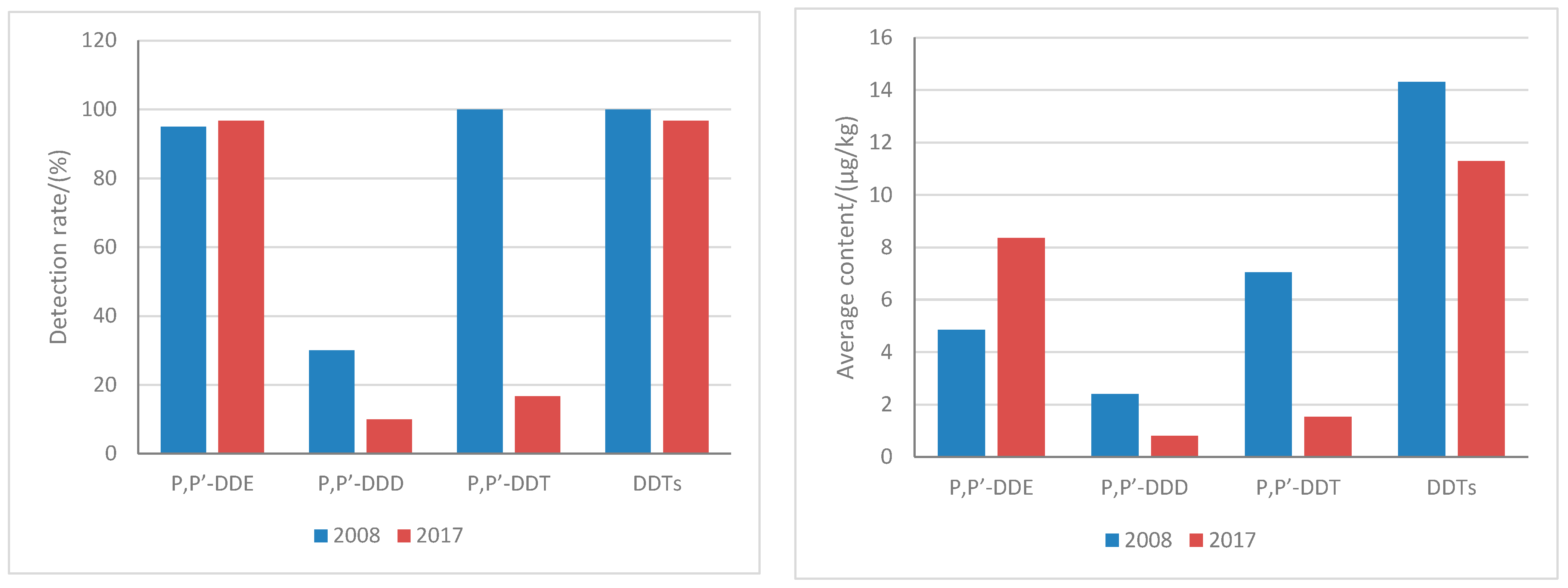
4.1.3. Characteristics of BHCs and DDTs in Soil
4.1.4. Characteristics of Endosulfan Sulfate and Hexachlorobenzene in Soil
4.2. OCPs in Groundwater
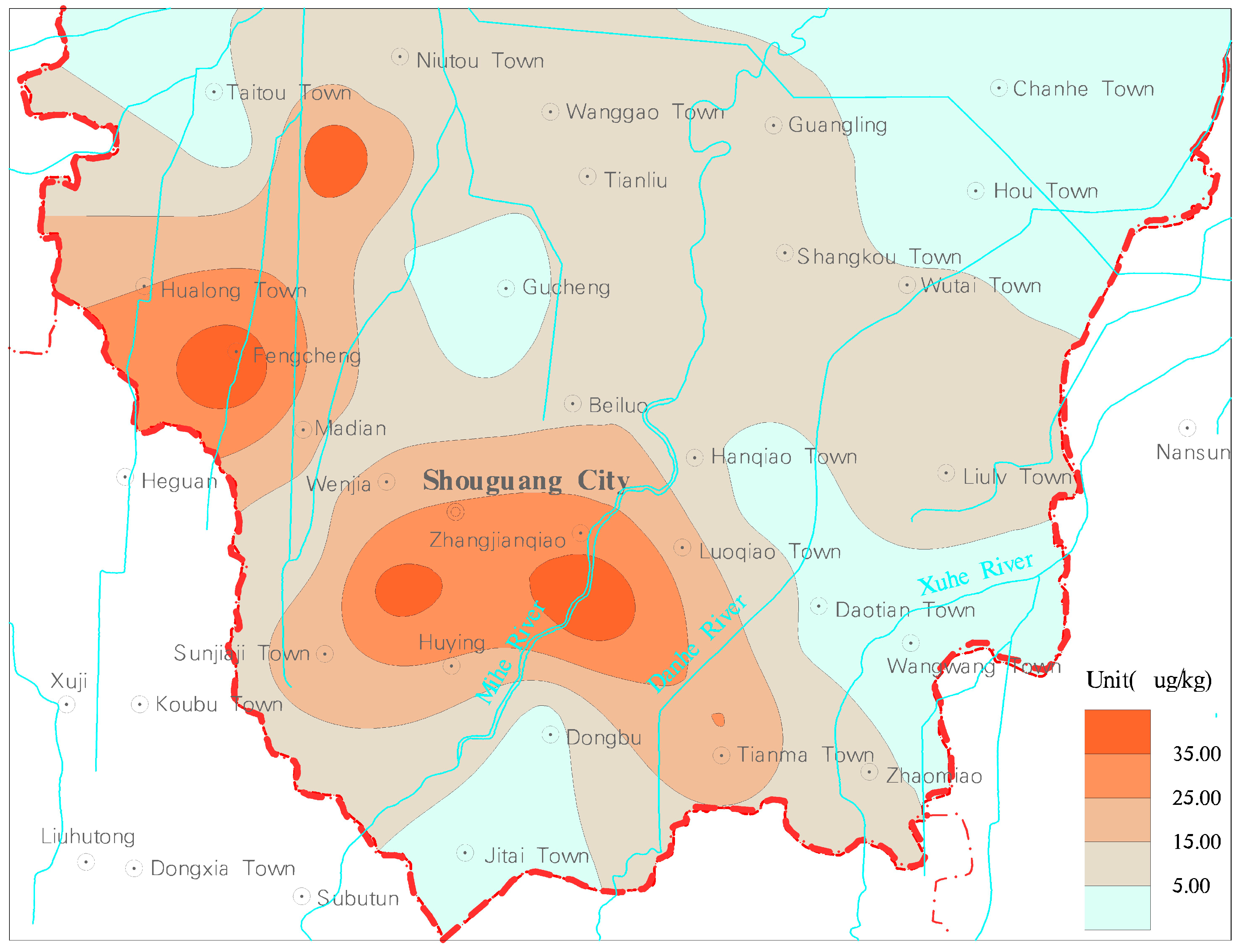
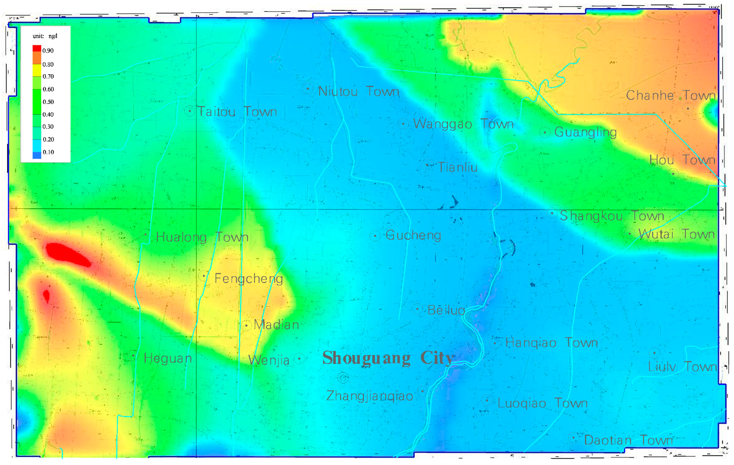
4.2.1. Distribution Characteristics of HCHs in Shallow Groundwater
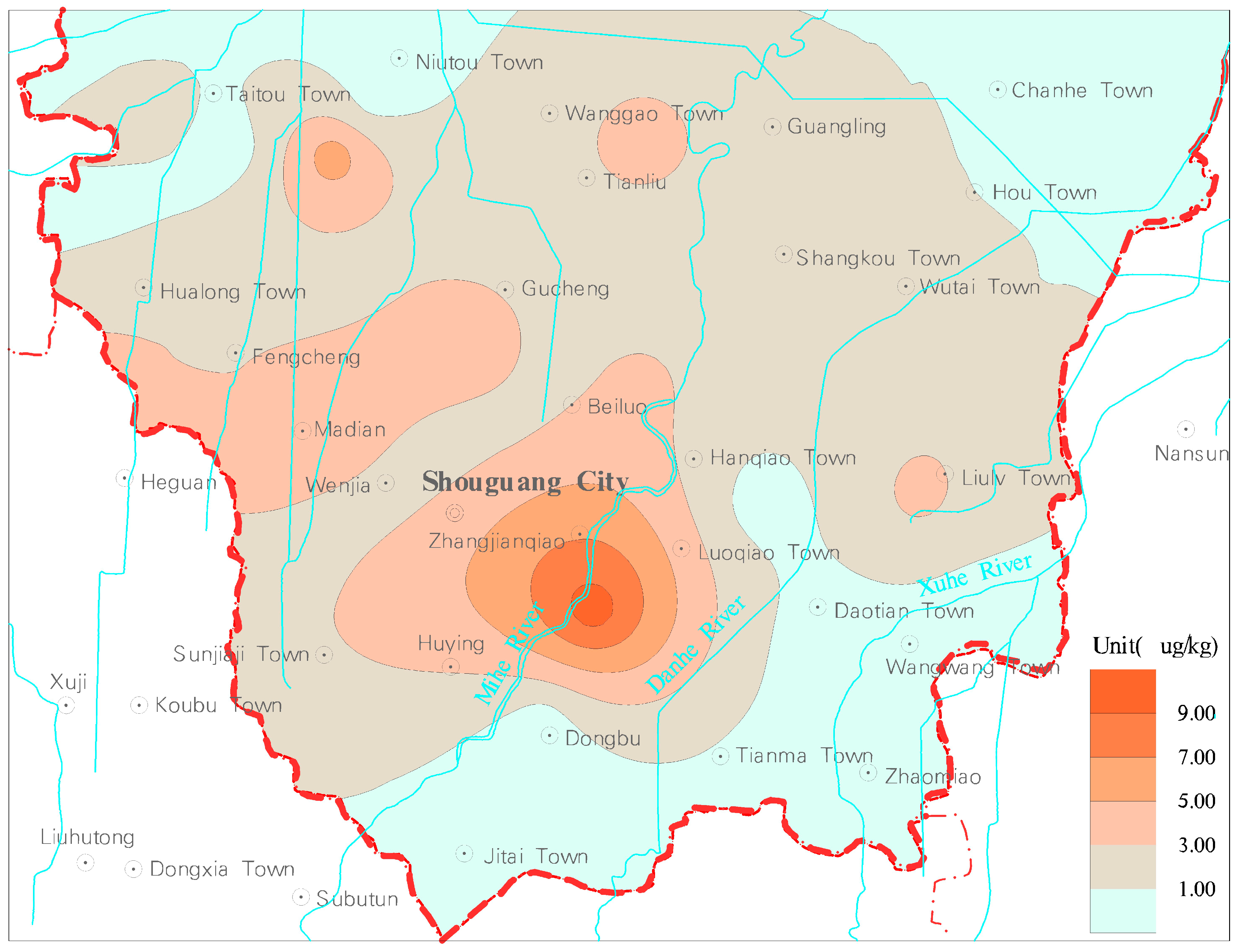
4.2.2. Distribution Characteristics of DDTs in Shallow Groundwater
4.2.3. Distribution Characteristics of Endosulfate in Shallow Groundwater
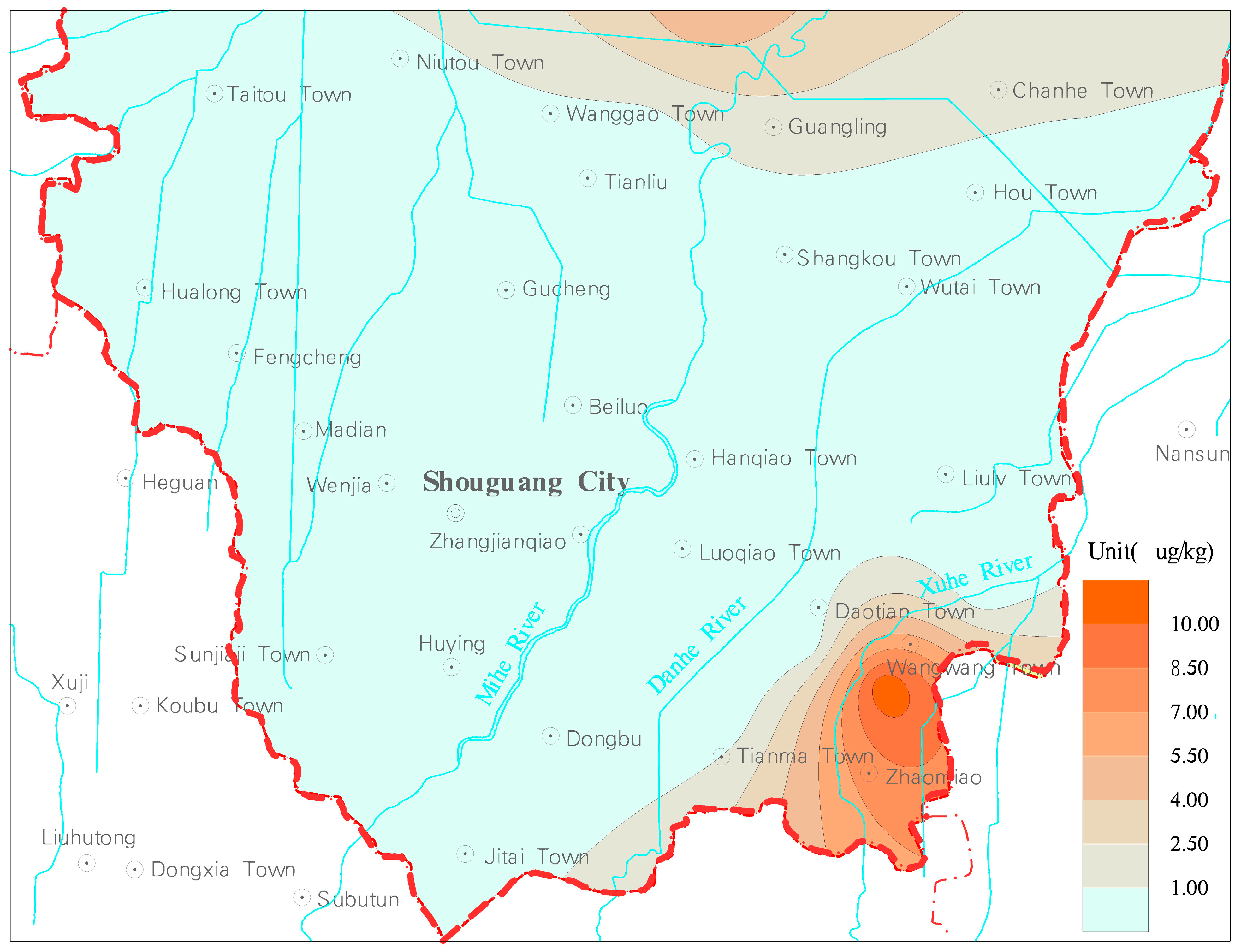
4.2.4. Distribution Characteristics of Hexachlorobenzene in Shallow Groundwater
4.3. Distribution Characteristics of Organochlorine Pesticides in Vegetables
4.3.1. Detection of Organochlorine Pesticides in Vegetables
4.3.2. Distribution Characteristics of Organochlorine Pesticides in Vegetables
4.4. Migration of OCPs in Soil-Groundwater
4.4.1. Prediction of Groundwater Migration in HCHs
4.4.2. DDTs Prediction Result
4.4.3. Prediction Results of Endosulfan Sulfate
4.4.4. Prediction Results of Hexachlorobenzene
5. Conclusions
Author Contributions
Funding
Data Availability Statement
Acknowledgments
Conflicts of Interest
References
- Kamalesh, T.; Kumar, P.S.; Rangasamy, G. An insights of organochlorine pesticides categories, properties, eco-toxicity and new developments in bioremediation process. Environ. Pollut. 2023, 333, 122114. [Google Scholar]
- Xu, C.; Cai, Y.; Wang, R.; Wu, J.; Yang, G.; Lv, Y.; Liu, D.; Deng, Y.; Zhu, Y.; Zhang, Q.; et al. Reduced attention on restricted organochlorine pesticides, whereas still noteworthy of the impact on the deep soil and groundwater: A historical site study in southern China. Environ. Geochem. Health 2023, 45, 8787–8802. [Google Scholar] [CrossRef] [PubMed]
- Tang, C.; Chen, Z.; Huang, Y.; Solyanikova, I.P.; Mohan, S.V.; Chen, H.; Wu, Y. Occurrence and potential harms of organochlorine pesticides (OCPs) in environment and their removal by periphyton. Crit. Rev. Environ. Sci. Technol. 2023, 53, 1957–1981. [Google Scholar] [CrossRef]
- Hassan, A. Perennial Existence of Organochlorine Pesticides in the Soils of Amghara, Kuwait. Bull. Environ. Contam. Toxicol. 2023, 111, 17. [Google Scholar]
- Hao, S.; Li, W.L.; Liu, L.Y.; Zhang, Z.F.; Ma, W.L.; Li, Y.F. Spatial distribution and temporal trend of organochlorine pesticides in Chinese surface soil. Environ. Sci. Pollut. Res. Int. 2023, 30, 82152–82161. [Google Scholar] [CrossRef] [PubMed]
- Muhammed, H.A.; Yahaya, A.; Abdullahi, S.S.; Jagaba, A.H.; Birniwa, A.H. Mitigating water contamination by controlling anthropogenic activities of organochlorine pesticides (OCPs) for surface water quality assurance. Case Stud. Chem. Environ. Eng. 2023, 8, 100474. [Google Scholar] [CrossRef]
- Yin, X.; Li, X.; Zhu, D.; Wang, H.; Li, X.; Yue, S.; Li, A. Residue characteristics, spatiotemporal distribution and ecotoxicological risk assessment of organochlorine pesticides and organophosphorus pesticides in surface water in Northwest Tai Lake Basin. Acta Sci. Circumst. 2023, 7, 1–16. [Google Scholar] [CrossRef]
- Lohmann, R.; Vrana, B.; Muir, D.; Smedes, F.; Sobotka, J.; Zeng, E.Y.; Bao, L.J.; Allan, I.J.; Astrahan, P.; Barra, R.O.; et al. Passive-Sampler-Derived PCB and OCP Concentrations in the Waters of the World—First Results from the AQUA-GAPS/MONET Network. Environ. Sci. Technol. 2023, 57, 9342–9352. [Google Scholar] [CrossRef]
- Guo, J.; Chen, W.; Wu, M.; Qu, C.; Sun, H.; Guo, J. Distribution, Sources, and Risk Assessment of Organochlorine Pesticides in Water from Beiluo River, Loess Plateau, China. Toxics 2023, 11, 496. [Google Scholar] [CrossRef]
- Cecchetto, F.; Villalba, A.; Vazquez, N.D.; Ramirez, C.L.; Maggi, M.D.; Miglioranza, K.S. Occurrence of chlorpyrifos and organochlorine pesticides in a native bumblebee (Bombus pauloensis) living under different land uses in the southeastern Pampas, Argentina. Sci. Total Environ. 2023, 905, 167117. [Google Scholar] [CrossRef]
- Capella, R.; Guida, Y.; Loretto, D.; Weksler, M.; Meire, R.O. Occurrence of legacy organochlorine pesticides in small mammals from two mountainous National Parks in southeastern Brazil. Emerg. Contam. 2023, 9, 100211. [Google Scholar] [CrossRef]
- Kumah, E.K.; Arah, I.K.; Anku, E.K.; Akuaku, J.; Aidoo, M.K. Determination of levels of organochlorine pesticide residues in some common grown and consumed vegetables purchased from Ho Municipal markets, Ghana. Cogent Food Agric. 2023, 9, 2191810. [Google Scholar] [CrossRef]
- Munjanja, B.K.; Nomngongo, P.N.; Mketo, N. Organochlorine pesticides in vegetable oils: An overview of occurrence, toxicity, and chromatographic determination in the past twenty-two years (2000–2022). Crit. Rev. Food Sci. Nutr. 2023, 1–17. [Google Scholar] [CrossRef] [PubMed]
- Sasaki, N.; Morse, G.; Jones, L.; Carpenter, D.O. Effects of mixtures of polychlorinated biphenyls (PCBs) and three organochlorine pesticides on cognitive function differ between older Mohawks at Akwesasne and older adults in NHANES. Environ. Res. 2023, 236 Pt 2, 116861. [Google Scholar] [CrossRef] [PubMed]
- Salimi, F.; Asadikaram, G.; Ashrafi, M.R.; Nejad, H.Z.; Abolhassani, M.; Abbasi-Jorjandi, M.; Sanjari, M. Organochlorine pesticides and epigenetic alterations in thyroid tumors. Front. Endocrinol. 2023, 14, 1130794. [Google Scholar] [CrossRef] [PubMed]
- Wei, H.; Lin, G.; Yao, X.; Li, J.; Wang, S.; Gong, X.; Cai, Y.; Zhang, L.; Zhao, Z. Sediment occurrence and risk of organochlorine pesticides in the surface water environment of Jiangsu in a typical plain river network area. China Environ. Sci. 2023, 43, 1–13. [Google Scholar] [CrossRef]
- Wang, L.; Cao, G.; Liu, L.Y.; Zhang, Z.F.; Jia, S.M.; Fu, M.Q.; Ma, W.L. Cross-regional scale studies of organochlorine pesticides in air in China: Pollution characteristic, seasonal variation, and gas/particle partitioning. Sci. Total Environ. 2023, 904, 166709. [Google Scholar] [CrossRef]
- Khuman, S.N.; Park, M.K.; Kim, H.J.; Hwang, S.M.; Lee, C.H.; Choi, S.D. Nationwide assessment of atmospheric organochlorine pesticides over a decade during 2008–2017 in South Korea. Sci. Total Environ. 2023, 877, 162927. [Google Scholar] [CrossRef]
- Li, S.; Zhang, Y.; Cong, B.; Liu, S.; Liu, S.; Mi, W.; Xie, Z. Spatial distribution, source identification and flux estimation of polycyclic aromatic hydrocarbons and organochlorine pesticides in basins of the Eastern Indian Ocean. Sci. Total Environ. 2023, 905, 166974. [Google Scholar] [CrossRef]
- Vudamala, K.; Chakraborty, P.; Chatragadda, R.; Tiwari, A.K.; Qureshi, A. Distribution of organochlorine pesticides in surface and deep waters of the Southern Indian Ocean and coastal Antarctic waters. Environ. Pollut. 2023, 321, 121206. [Google Scholar] [CrossRef]
- Xuan, Z.; Ma, Y.; Zhang, J.; Zhu, J.; Cai, M. Dissolved legacy and emerging organochlorine pesticides in the Antarctic marginal seas: Occurrence, sources and transport. Mar. Pollut. Bull. 2022, 187, 114511. [Google Scholar] [CrossRef] [PubMed]
- Wang, C.; Feng, L.; Thakuri, B.; Chakraborty, A. Ecological risk assessment of organochlorine pesticide mixture in South China Sea and East China Sea under the effects of seasonal changes and phase-partitioning. Mar. Pollut. Bull. 2022, 185 Pt A, 114329. [Google Scholar] [CrossRef]
- Zheng, H.; Ding, Y.; Xue, Y.; Xiao, K.; Zhu, J.; Liu, Y.; Cai, M. Occurrence, seasonal variations, and eco-risk of currently using organochlorine pesticides in surface seawater of the East China Sea and Western Pacific Ocean. Mar. Pollut. Bull. 2022, 185 Pt A, 114300. [Google Scholar] [CrossRef]
- Sim, W.; Nam, A.; Lee, M.; Oh, J.E. Polychlorinated biphenyls and organochlorine pesticides in surface sediments from river networks, South Korea: Spatial distribution, source identification, and ecological risks. Environ. Sci. Pollut. Res. Int. 2023, 30, 94371–94385. [Google Scholar] [CrossRef] [PubMed]
- Chuanhai, H.; Yuqiang, T. Spatial-temporal occurrence and sources of organochlorine pesticides in the sediments of the largest deep lake (Lake Fuxian) in China. Environ. Sci. Pollut. Res. Int. 2023, 30, 31157–31170. [Google Scholar]
- Zhao, X.; Chen, L.; Guo, W.; Lu, S. Temporal trends, sources, and ecological risk of residual organochlorine pesticides (OCPs) in sediment core from the Dongping Lake, North China. Environ. Sci. Pollut. Res. Int. 2023, 30, 103033–103043. [Google Scholar] [CrossRef] [PubMed]
- Ma, Y.; Xu, T.; Mao, Q.; Zhou, X.; Wang, R.; Sun, J.; Zhang, A.; Zhou, S. Distribution and flux of organochlorine pesticides in sediment from Prydz Bay, Antarctic: Implication of sources and trends. Sci. Total Environ. 2021, 799, 149380. [Google Scholar] [CrossRef]
- Zhang, J.; Sun, W.; Shi, C.; Li, W.; Liu, A.; Guo, J.; Zheng, H.; Zhang, J.; Qi, S.; Qu, C. Investigation of organochlorine pesticides in the Wang Lake Wetland, China: Implications for environmental processes and risks. Sci. Total Environ. 2023, 898, 165450. [Google Scholar] [CrossRef]
- Mamontova, E.A.; Mamontov, A.A. Spatial and Temporal Variations of Polychlorinated Biphenyls and Organochlorine Pesticides in Snow in Eastern Siberia. Atmosphere 2022, 13, 2117. [Google Scholar] [CrossRef]
- Veludo, A.F.; Figueiredo, D.M.; Degrendele, C.; Masinyana, L.; Curchod, L.; Kohoutek, J.; Kukučka, P.; Martiník, J.; Přibylová, P.; Klánová, J.; et al. Seasonal variations in air concentrations of 27 organochlorine pesticides (OCPs) and 25 current-use pesticides (CUPs) across three agricultural areas of South Africa. Chemosphere 2021, 289, 133162. [Google Scholar] [CrossRef]
- Tesfaye, B.; Gure, A.; Asere, T.G.; Molole, G.J. Deep eutectic solvent-based dispersive liquid–liquid microextraction for determination of organochlorine pesticides in water and apple juice samples. Microchem. J. 2023, 195, 109428. [Google Scholar] [CrossRef]
- Dar, A.A.; Jan, I.; Shah, M.D.; Sofi, J.A.; Hassan, G.I.; Dar, S.R. Monitoring and method validation of organophosphorus/organochlorine pesticide residues in vegetables and fruits by gas chromatography. Biomed. Chromatogr. BMC 2023, e5756. [Google Scholar] [CrossRef] [PubMed]
- Hoseinzadeh, A.; Heidari, H.; Matin, A.A.; Soylak, M. Multi-response optimization of a deep eutectic solvent-based microextraction method for the simultaneous extraction of twenty organochlorine pesticides for monitoring in various water samples. Microchem. J. 2023, 194, 109226. [Google Scholar] [CrossRef]
- Zhou, Y.; Pan, S. Assessment of the efficiency of immobilized degrading microorganisms in removing the organochlorine pesticide residues from agricultural soils. Environ. Monit. Assess. 2023, 195, 1274. [Google Scholar] [CrossRef] [PubMed]
- Martin, D.E.; Alnajjar, P.; Muselet, D.; Soligot-Hognon, C.; Kanso, H.; Pacaud, S.; Le Roux, Y.; Saaidi, P.L.; Feidt, C. Efficient biodegradation of the recalcitrant organochlorine pesticide chlordecone under methanogenic conditions. Sci. Total Environ. 2023, 903, 166345. [Google Scholar] [CrossRef] [PubMed]
- Cui, H.; Zeng, J.; Ren, Y.; Liu, H.; Deng, R.; Zhang, W.; Lv, Y.; Wan, Q.; Yang, L.; Liu, P.; et al. Theoretical studies on the degradation mechanism of organochlorine pesticides in the presence of Si-OH in sepiolite. J. Mol. Struct. 2023, 1279, 134955. [Google Scholar] [CrossRef]
- Wang, L.; Zhang, Z.F.; Liu, L.Y.; Zhu, F.J.; Ma, W.L. National-scale monitoring of historic used organochlorine pesticides (OCPs) and current used pesticides (CUPs) in Chinese surface soil: Old topic and new story. J. Hazard. Mater. 2022, 443 Pt B, 130285. [Google Scholar] [CrossRef]
- Cárdenas, S.; Márquez, A.; Guevara, E. Diffusion–advection process modeling of organochlorine pesticides in rivers. J. Appl. Water Eng. Res. 2023, 11, 1–22. [Google Scholar] [CrossRef]
- Márquez-Romance, A.; Cárdenas-Izaguirre, S.; Guevara-Pérez, E.; Pérez-Pacheco, S. Calibration of diffusion-advection process models for organochlorine pesticides in a tropical river. Environ. Qual. Manag. 2021, 31, 403–424. [Google Scholar] [CrossRef]
- Li, C.; Liu, Z.; Liu, Y.; Zhang, J.; Meng, Q.; Xiao, Y.; Liu, L.; Chen, Z.; Wang, F.; Huang, H. Study on the Migration Law of Organic Chlorine in Soil-Groundwater in Typical Agricultural Production Areas; Shandong GEO-Surveying & Mapping Institute: Ji’nan, China, 2017. [Google Scholar]


| Area | Mean Content/(μg/kg) | |||
|---|---|---|---|---|
| HCHs | DDTs | Endosulfan Sulfate | Hexachlorobenzene | |
| Huanghe River Basin | 1.23~8.29 (6.23) | 2.56~42.41 (16.78) | 0.78~8.15 (5.12) | |
| Jianghan Plain | 0.85~7.06 | 12.28~415.80 | 0.16~3.78 (0.90) | 0.10~15.38 (1.15) |
| Suburb of Shengyang | 0.67–224.51 (14.51) | 0.99~218.56 (25.28) | 0.54~41.65 (8.35) | |
| Leizhou Peninsula | nd~65.93 (3.43) | nd~52.00 (3.83) | nd~7.66 (1.48) | |
| Zaozhuang City (Agricultural soil) | 21.9~26.9 (25.1) | 43.9~64.8 (54.8) | ||
| Liaocheng (cultivated land soil) | nd~52.25 (11.16) | nd~4451.06 (127.75) | nd~13.72 (2.48) | |
| Yantai city | 26~561 (165) | 10~2660 (160) | ||
| Dongying (Yellow River Estuary) | 0.28–1.32 (0.345) | 0.17~10.46 (0.634) | nd~0.58 (0.19) | |
| Qingdao city | 0.41~9.67 (4.01) | 3.88~79.55 (26.51) | ||
| The study area | nd~18.64 (1.44) | nd~45.33 (11.28) | nd~128.49 (18.45) | nd~11.54 (1.56) |
Disclaimer/Publisher’s Note: The statements, opinions and data contained in all publications are solely those of the individual author(s) and contributor(s) and not of MDPI and/or the editor(s). MDPI and/or the editor(s) disclaim responsibility for any injury to people or property resulting from any ideas, methods, instructions or products referred to in the content. |
© 2023 by the authors. Licensee MDPI, Basel, Switzerland. This article is an open access article distributed under the terms and conditions of the Creative Commons Attribution (CC BY) license (https://creativecommons.org/licenses/by/4.0/).
Share and Cite
Li, C.; Qi, X.; Wang, Y.; Meng, Q.; Li, W.; Liu, L.; Zheng, Y.; Cui, H. Organochlorine Pesticides in Soil–Groundwater–Plant System in a Famous Agricultural Production Area in China: Spatial Distribution, Source Identification and Migration Prediction. Water 2023, 15, 4147. https://doi.org/10.3390/w15234147
Li C, Qi X, Wang Y, Meng Q, Li W, Liu L, Zheng Y, Cui H. Organochlorine Pesticides in Soil–Groundwater–Plant System in a Famous Agricultural Production Area in China: Spatial Distribution, Source Identification and Migration Prediction. Water. 2023; 15(23):4147. https://doi.org/10.3390/w15234147
Chicago/Turabian StyleLi, Chuansheng, Xiaofan Qi, Yu Wang, Qingjie Meng, Wenpeng Li, Lanyu Liu, Yuejun Zheng, and Huqun Cui. 2023. "Organochlorine Pesticides in Soil–Groundwater–Plant System in a Famous Agricultural Production Area in China: Spatial Distribution, Source Identification and Migration Prediction" Water 15, no. 23: 4147. https://doi.org/10.3390/w15234147
APA StyleLi, C., Qi, X., Wang, Y., Meng, Q., Li, W., Liu, L., Zheng, Y., & Cui, H. (2023). Organochlorine Pesticides in Soil–Groundwater–Plant System in a Famous Agricultural Production Area in China: Spatial Distribution, Source Identification and Migration Prediction. Water, 15(23), 4147. https://doi.org/10.3390/w15234147