Abstract
Transitional free surface flow profiles with a critical point occur with weak vorticity and viscosity effects and thus can be modeled with an irrotational flow approach. Important examples in hydraulic engineering include flow over low obstacles, transition structures in canals, and flow over high spillways. While solving Laplace’s equation is relatively simple, the determination of the unknown free surface and energy head of the flow is challenging. Both hydraulic quantities need to be iterated before solving the Laplace equation. Former models iterated the energy head on a trial-and-error basis, assuming that the linked free surface profile is smooth, i.e., free of waves. The iteration of the free surface for a given head is frequently accomplished using the Newton–Rapshon method, which is difficult for the challenging case of spillway flow, giving no solution in some cases. An alternative method of computing irrotational flow profiles in transitional flows involving a critical point is proposed in this work. The model contains three elements: mapping of Laplace’s equation to directly track the streamlines, determination of the critical point and unknown energy head using a critical flow condition for irrotational flows, and determination of the water surface position using an exact analytical solution. The proposed model is favorably compared with experimental data from different sources and CFD results, indicating a reasonable agreement.
1. Introduction
The determination of open channel flow in transitions involving a critical point, i.e., where the flow changes from upstream subcritical to downstream supercritical flow conditions, involves weak vorticity and viscous effects, and it is thus well approximated as irrotational flow [1,2,3,4,5,6]. Important examples in hydraulic engineering include weirs for discharge measurement [7], transition structures in canals, and the spillway of high dams [8,9,10] (Figure 1), which are typical cases among the more complex problems in this field.
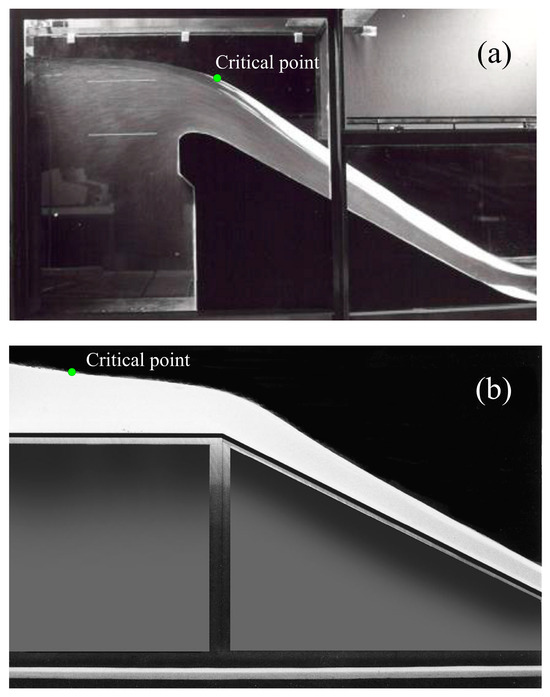
Figure 1.
Irrotational open channel flows with a critical point (a) flow over an ogee crest, (b) transition from mild to steep slope (photos by W.H. Hager).
The solution of the irrotational spillway flow problem is not simple and entails three iteration blocks. First, for a given discharge, the energy head H is unknown; thus, it is necessary to start with a guessed energy head and iterate it. Second, for a given energy head, it is necessary to iterate the position of the free surface to make the pressure head zero at all the free surface nodes, thereby rendering the energy in these nodes equal to the assumed energy head. Third, for the guessed energy head and iterated surface position, the Laplace equation must be solved to produce a velocity field solution.
The iteration of Laplace’s equation is not usually a problem, but energy head and free surface iterations are not simple. Many models iterate H by the trial-and-error approach, after inspection of the iterated free surface for this head and deciding if it is physically reasonable, i.e., free of oscillations. The iteration of the free surface for a given H is typically achieved by a Newton–Rapshon-type method. This procedure is delicate and may produce unphysical solutions or simply no solution. Iterating the head based on the success of the free surface iteration, i.e., on satisfying the zero-pressure condition, may result in a vicious loop not giving a solution at all, even working with high numerical accuracy. If the guessed energy head is far from its correct value, no solution to the problem may exist. Further, a train of unrealistic waves may be formed upstream of the crest, with the governing equations and boundary conditions satisfied in a numerical sense [11].
The solution of the Laplace equation for an irrotational velocity field is not difficult and can either be conducted in the physical plane or in other planes, such as the complex potential plane [12]. The elliptic problem can be solved by a variety of numerical methods [13]; obtaining an accurate solution is feasible with simple means. Solution methods in the literature include the finite difference method [12,14,15,16,17,18], the finite element method [19,20,21,22,23,24,25,26], and the boundary element method [27,28,29]. The determination of the critical point, the energy head of irrotational flow, and the water surface profile for a given discharge is, however, not simple. An accepted method has been to use trial values of H until the flow profile obtained is as smooth as possible [11,26]. Methods dealing with the free surface boundary condition consisted, basically, in satisfying the Bernoulli equation by setting the pressure head to zero at the upper boundary. The discrete version of Bernoulli’s equation was then used to move the free surface iteratively based on the Newton–Raphson method. The solution process is delicate, and a good initial surface profile is needed to start iterations, combined with a strong damping of the Newton–Raphson correction vector to make minute surface displacements [16,27]. Even taking care of both issues, success in the iteration process cannot be guaranteed. If the iteration of the water surface is successful, a new guessed value of H can be tried. Ideally, a physical criterion to iterate the head H is needed to progressively approximate it, simultaneously, while the free surface is iterated. This research focuses on this aspect of the problem. An updated discussion of the state of the art in irrotational open channel flow modeling is available in books by Castro-Orgaz and Hager [30,31] and Katopodes [13].
In this work, an alternative method of computing irrotational flow profiles in open-channel transitional flows is proposed. It consists in solving the Laplace equation using a mapping which transforms the computational domain into a rectangle, combined with a generalized definition of critical flow for two-dimensional irrotational flows, which automatically determines the critical point position and energy head of the flow. The sub- and supercritical portions of the water surface profile are determined with an exact analytical solution, allowing for a fast, robust, and accurate computation. The proposed method is validated by comparison with experiments for three relevant test cases: flow over low obstacles, the transition from mild to steep slopes, and flow over a spillway crest.
The value of the proposed method in practical engineering lies in the fact that the determination of the flow profiles is exact and fast using analytical equations, eliminating the stability issues of other methods, which may not converge into a physical solution. Scientifically, the method is based on the sound physical principle of critical flow generalized to rapidly varied irrotational flow. Instead, other methods are based purely on numerical tools, like the Newton–Raphson algorithm.
2. Irrotational Flow Modeling
2.1. The x-ψ Method
Consider steady irrotational flow over an uneven bed with a free surface (Figure 2). The flow depth measured vertically is h(x) and the rigid bed profile is zb(x), with x as the horizontal coordinate. The velocity components in Cartesian directions (x, z) are (u, w), and the total energy head of the flow is H. For irrotational and incompressible fluid flow, a stream function ψ defines the velocity components as [32,33]
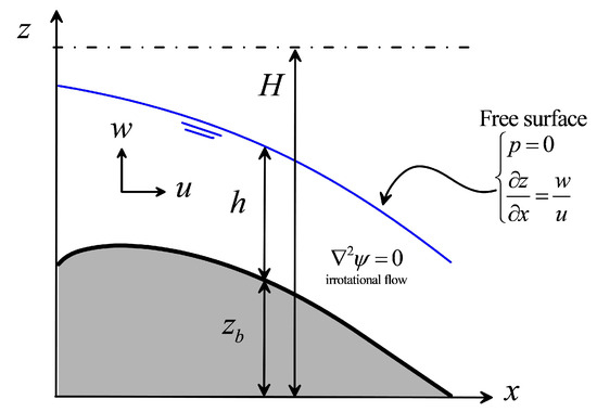
Figure 2.
Steady irrotational flow over a channel transition.
Interior flow bounded by the free surface and bed streamlines obeys the Laplace equation [34]
This equation solved in the physical plane (x, z) by a finite difference method [14,15,18] yields the velocity components by differentiation of the ensuing ψ function. The solution domain in this plane is irregular and it is, therefore, necessary to use special finite-difference formulae near the boundary streamlines to solve the equation. Alternatively, the finite element method has been employed, allowing for a flexible mesh fitted to the irregular flow domain [20,21,22,23].
Thom and Apelt [12] proposed to interchange the role of dependent and independent variables; thus, the variables (x, z) are determined as functions of (ϕ, ψ), where ϕ is the potential function. The Laplacians are expressed then as
In the complex potential plane (ϕ, ψ), the computational domain is a rectangular band requiring no irregular mesh, which is a major advantage of Thom and Apelt’s [12] development. Cassidy [35] adopted a solution procedure for standard spillway flow employing the logarithmic hodograph lnV + iθ, where the modulus of the velocity vector is V = (u2 + w2)1/2 and the streamline inclination tanθ = w/u. In the complex potential plane (ϕ, ψ), lnV and θ are harmonic functions; they must satisfy the Laplace equation, namely
Here, we will employ a similar procedure based on the x-ψ mapping, where the elevation is taken as a dependent variable of x and ψ, resulting in the Laplacian [16,17,36]
In the x-ψ plane, the computational domain for steady irrotational flow is also a rectangular band, thereby simplifying the solution procedure. Once Equation (8) is solved, the coordinates of the streamlines are available, i.e., z = z(x, ψ = const). The velocity component u is then determined using Equation (1) and the vertical component w by resorting to the streamline condition
Once the particle kinematics are resolved, the pressure p at any point of the flow is determined from the Bernoulli equation
2.2. Free Surface Boundary Condition
The free surface is a streamline where the pressure is atmospheric, i.e., p = 0. The Bernoulli equation then gives the free surface boundary condition as [30,32]
where subscript s refers to free surface, Vs is the absolute free surface velocity, and E is the specific energy of the free surface streamline. Some former models have directly used a finite difference version of Equation (11), to be satisfied in a numerical setting [16,17,27]. The process is far from simple for flows with a critical point, as will be discussed below. Here, we will transform Equation (11) to produce a more suitable form of this challenging boundary condition.
Following Wilkinson [37], we rewrite Equation (11) as follows:
Coefficient α is not the Coriolis coefficient, but simply the ratio of free surface to depth-averaged velocities. Now, we define the following scaling length
Using Equations (12) and (13), the specific energy of the free surface streamline reads in dimensionless form
Equation (14) can be written as follows [38]:
where
The two positive roots of a cubic-like of Equation (15) are [38,39]
for h > hc, and
for h < hc. Here
If hc is interpreted as a critical flow depth, then Equations (17) and (18) define sub- and supercritical flow profiles, respectively. Note that the solution is analytical and exact: so far, no approximations are invoked, given that no assumptions were made on the nature of coefficient α. Therefore, the solution is exact and can be employed to determine the irrotational flow profiles in open channel transitions. If α = 1, the flow is hydrostatic, and Equations (17) and (18) represent alternate depths in the specific energy diagram of gradually varied open channel flow [31,39,40,41].
2.3. Critical Point
In irrotational flow along an open channel transition with a change from upstream subcritical to downstream supercritical flow, the critical point is formed elsewhere. In general, this critical point is in a zone where streamlines are curved and sloped [3,4,5], which makes it hard to locate it. Fawer [42], Jaeger [43], and Dao-Yang [44] demonstrated that the critical flow concept widely used in gradually varied flows [40,45] can be generalized to two-dimensional irrotational flows. Thus, we define now the general critical flow conditions for these points. We determine critical flow from the minimum specific energy condition, resulting from Equation (12) in [37]
The resulting minimum specific energy is then
Equations (20) and (21) are fully general. An approximation is made now neglecting the variation of α with h, resulting for the critical point in the relations
For brevity, we use subindex c to refer to “critical” conditions henceforth. Thus, the flow depth at the critical point is given by Equation (13). This approximation was found to be accurate enough, as will be shown with ensuing computations. Note that 2D irrotational flow features are included in the critical flow condition trough the coefficient α.
3. Solution Method
The solution process entails three steps: First, for a known flow profile h(x), the Laplace Equation (8) is solved and the free surface velocity coefficient α(x) along the computational domain is determined. Then, the critical point and unknown energy head are estimated from Equations (22) and (23) [44]. Further, the sub- and supercritical flow profiles are analytically determined from the critical point in the up- and downstream directions, respectively, by resorting to Equations (17) and (18).
The Laplace Equation (8) is solved using a finite difference approximation in the x-ψ plane (Figure 3). This equation produces the shape of the streamlines in the physical plane (Figure 3a). The boundary conditions are as follows. By choice, the no-flow bottom boundary is assigned the value ψ = 0, whereas the free surface boundary corresponds to ψ = q, with q as the discharge per unit channel width. Inflow/outflow boundary conditions are in zones of nearly horizontal flow, where the variation of the stream function with elevation may be assumed to be linear, an assumption compatible with hydrostatic flow conditions. Equation (8) is discretized using second-order central finite differences in the mesh sketched in Figure 3b, and the resulting system of linear equations is solved by successive overrelaxation (SOR) method [13]. The discretization is described in detail by Montes [17] and Castro-Orgaz [46] and it is not repeated here. Once the stream function ψ is available in the entire computational domain, the velocities (u, w) are computed by second-order finite difference approximations of Equations (1) and (9). This permits us to compute α in each free surface node of the mesh.
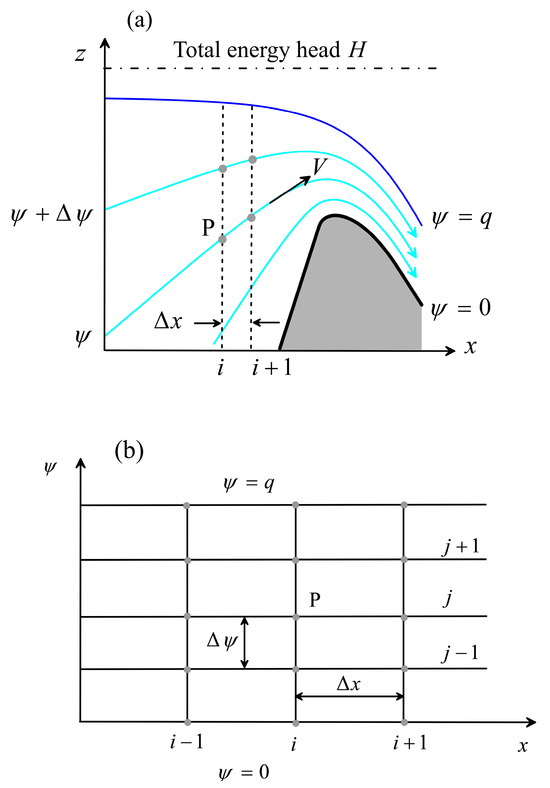
Figure 3.
Numerical discretization: (a) physical plane, (b) computational plane.
The next step is to obtain a new estimation of H. The algorithm to determine the critical point and total energy head is as follows. Assume an estimation of the flow profile h(i) is available along with the surface coefficients α(i). Following Jaeger [47] and Dao-Yang [44], it is possible to define a critical depth profile along the channel, given by
Now, the minimum specific energy at each channel section reads
This minimum specific energy can be transformed into the minimum total energy head at each node as follows:
This computation yields the minimum total head necessary at each node of the mesh for the discharge q; thus, at each node, a physical solution implies H ≥ Hmin(i). The maximum value of this set will satisfy this requirement at each free surface node, resulting in the new head estimation [44]
This fixes the position of the critical point in the mesh, icritical, and a new estimation of the total energy head of the flow.
Now, with the local free surface specific energy at each node given by E(i) = H − zb(i), the flow profile
is computed for subcritical flow (i < icritical), and the branch
applies for supercritical flow (i > icritical), where
For the new free surface position obtained with Equations (28) and (29), the pressure residual at each free surface node is determined by a finite difference approximation of Equation (10).
The computational process can be summarized as follows:
- Select a discharge q;
- Determine the critical point and total energy head H. Start assuming α(i) = 0 (initial hydrostatic flow profile);
- Compute the sub- and supercritical portions of the flow profile using Equations (28) and (29);
- For the new free surface position, solve the Laplace equation by SOR and compute a new set of coefficients α(i) at each node on the free surface;
- Compute the free surface pressure residuals. If their average is not below a tolerance, go back to 2 and start a new free surface iteration.
Step 2 of the algorithm uses an initial profile which is not accurate. However, as will be specifically discussed in the ogee spillway test (see Section 4.3), the method progressively converges to the correct solution, not resulting in a source of error. Step 3 is a very fast and simple part of the algorithm, involving analytical equations which reduce, therefore, the limitations and uncertainties present in purely numerical methods based on iterating the free surface position by a Newton–Raphson algorithm. Step 4 of the algorithm involves the solution of a well-posed elliptic problem, which generally converges. However, to obtain an accurate solution in zones of rapidly varied flows, a low tolerance is advisable, e.g., 10−12 is suggested. Otherwise, the computed velocity field may not be accurate enough, such as in flow over an ogee weir.
The current approach diverges from former methods by Dao-Yang [44], Jaeger [47], Montes [16,17], and Castro-Orgaz [46], but combines some of the best elements of them: In the works of Jaeger [47] and Castro-Orgaz [46], the concept of critical flow in 2D irrotational motion is used, but it is assumed that the critical point is at the weir crest, whereas the current method determines the real critical point position as part of the problem solution. Montes [16,17] and Castro-Orgaz [46] used a x-ψ mapping but determined the free surface position by a purely numerical method, which fails to converge when curvilinear effects are high. In contrast, the proposed determination of the flow profile in the current work is analytical and was found to be convergent in all cases. Dao-Yang [44] determined the critical point position and free surface by setting small displacements of the length of the equipotential curves. In our proposed method, the critical point position is determined similarly to Dao-Yang [44], but we computed the free surface position analytically with our generalization of the specific energy based on the form of Bernoulli equation as proposed by Wilkinson [37].
4. Test Cases
Three test cases of increasing complexity are analyzed to validate the approximation proposed. The first involves flows over low obstacles of symmetrical and asymmetrical shape [48,49,50], where dynamic pressures remain positive. The energy head is unknown in advance, but the critical point is close to the crest. The second test is the transition from mild to steep slopes [17,43,51,52,53]. In this test, the critical point is fixed at the inlet and the energy head is known. However, dynamic pressures become negative due to the strong curvature at the transition, in addition to the chute steep slope effect. Finally, the most stringent test case is flow over an ogee crest [54,55,56,57,58], where dynamic pressures become negative for heads above design. The energy head, and thus the discharge coefficient, is unknown in advance, and due to the strong variation of bed curvature, the critical point is significantly shifted away from the spillway crest [48,59].
4.1. Flow over Low Humps
Sivakumaran et al.’s [49] experiments of flows over obstacles in a horizontal flume 0.915 m long, 0.65 m high, and 0.30 m wide are considered in Figure 4 and Figure 5. Two types of bed profiles were considered: symmetrical and asymmetrical. Figure 4 contains the experimental free surface and bed pressure head profiles for flow over an asymmetrical bed profile designed using B-Splines [50]. The unit discharge for this test is q = 0.11165 m2/s.
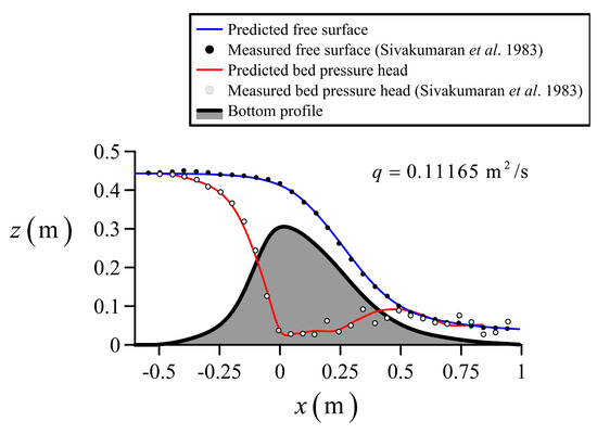
Figure 4.
Flow over an asymmetrical bed profile: comparison of irrotational flow model with experiments [49].
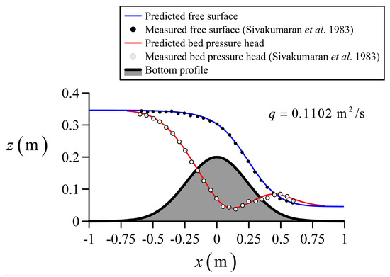
Figure 5.
Flow over a symmetrical bed profile: comparison of irrotational flow model with experiments [49].
Simulation with the irrotational flow model was accomplished using ∆x = 0.01 m and 20 streamlines. To obtain an accurate solution, tolerance in the SOR solver was set to 10−12. The overrelaxation coefficient was set to 1.8. To increase stability, the new free surface position was taken as the average of the former and new estimations achieved in each iteration. Overall, after 20–25 iterations, the free surface was estimated with enough accuracy. During the solution, it was observed that small wiggles formed near the estimated critical point. On tracking the numerical solution in detail, this was produced by small oscillations of the surface velocity near the critical point. These surface velocity oscillations were produced by the Laplace solver in response to curvature discontinuities in the free surface boundary resulting when assembling Equations (28) and (29) at the critical point. An expansion of the velocity field near the free surface reveals that (u, w) are functions of the water depth derivatives hx, hxx, hxxx… [6,60]. This explains the observed behaviour during the solution procedure. A Savitzky–Golay smoothing filter was then applied to remove these oscillations at the critical point. Note from Figure 4 that the solution produced is in excellent agreement with the observations, resulting in an accurate transitional flow profile from sub- to supercritical flows. The average residual pressure on the free surface for this solution is 2 × 10⁻⁴ m. The critical point is at x = 0.04 m, whereas the crest is at x = 0.02 m, i.e., there is a shift in the downstream direction, albeit small. The impact of filtering on the accuracy and reliability of results was double checked by comparing this test solution with that determined with the method by Castro-Orgaz [46], resulting in imperceptible differences. For high curvature effects, like those in the ogee crest (Section 4.3), the method by Castro-Orgaz [46] failed to produce a solution, whereas the current method produced a solution in conformity with experiments and CFD results, thereby ensuring that the filtering effects only stabilized without any impact on the physical accuracy of the solutions produced (see Section 4.3).
Figure 5 contains the experimental free surface and bed pressure head profiles for flow over a symmetrical bed profile of equation zb = 0.2exp[−0.5(x/0.24)2] (m) [49]. The unit discharge for this test is q = 0.1102 m2/s. The parameters in the numerical model were kept unaltered, and the resulting free surface and bed pressure head profiles are plotted in Figure 5. For this test, the irrotational flow solution is also in excellent agreement with observations.
4.2. Flow Transition from Mild to Steep Slopes
Figure 6 and Figure 7 consider the transition from mild to steep slopes [17,51], experimentally investigated by Hasumi [61]. In his set-up, an approaching critical flow accelerates over a horizontal flume towards a transitional curve designed with a circular arc of radius 0.1 m, which is tangent to downstream ramps of 45° and 60°. The flume width is 0.4 m and discharges of 20, 40, and 60 L/s were considered for the two chute slopes. The free surface and piezometric pressure profiles obtained by Hasumi [61] are plotted in Figure 6 and Figure 7. Observe the negative pressures in the transition arc for all tests. The critical point is fixed at the channel inlet, with a flow depth of hc = (q2/g)1/3. The energy head is thus known and of value H = (3/2)hc. Simulation with the irrotational flow model was accomplished using ∆x = 0.005 m and 20 streamlines to adequately capture the pressure drop in the transition zone. Further refinement of the mesh did not produce better results. For the 45° chute slope, the irrotational flow results presented in Figure 6 are in excellent agreement both for the free surface and piezometric pressure profiles for the three discharges tested. Note the non-hydrostatic bottom pressure on the chute slope. Simulations for the 60° slope presented in Figure 7 also reveal excellent free surface predictions. However, piezometric bed pressure profiles for 20 and 40 L/s show an appreciable distortion as compared to experiments. For 60 L/s, the prediction is in better agreement with the observations. The reason for the discrepancy at 20 and 40 L/s is unknown. It could be due to flow separation. However, no definite statement can be made in this regard, and it can only be said that the irrotational flow model prediction is in fair agreement with observations for the 60° chute flow test.
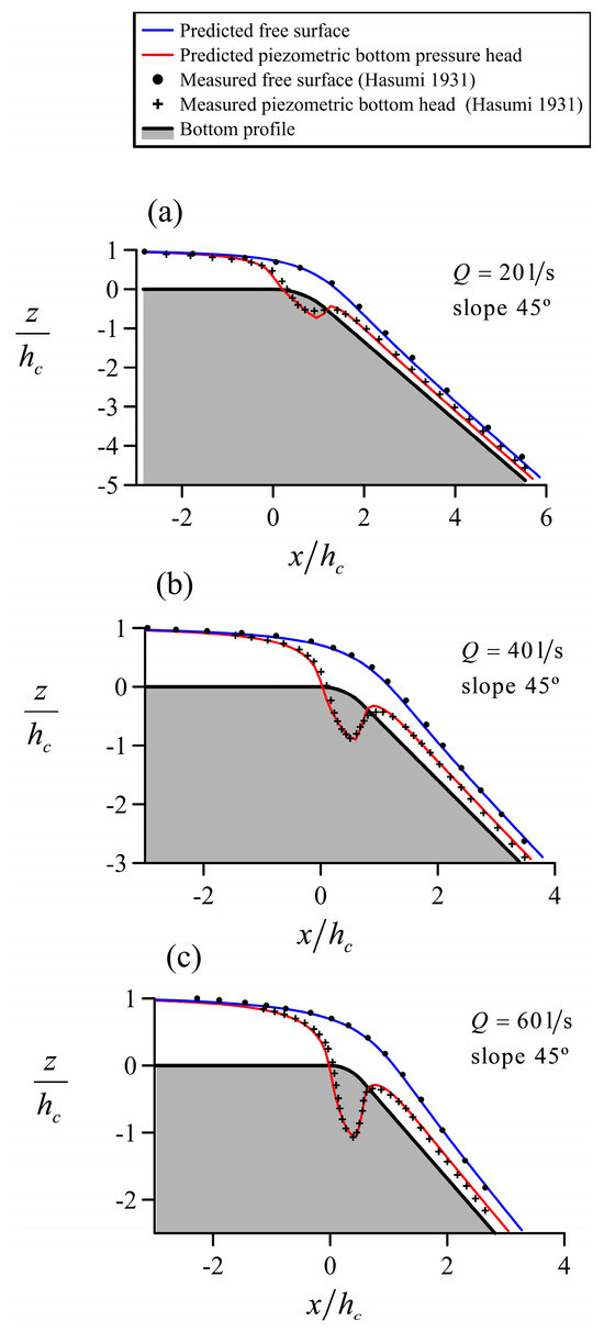
Figure 6.
(a–c) Flow in transition of horizontal channel to 45°: comparison of irrotational flow model with experiments [61]. The scaling used is hc = (q2/g)1/3.
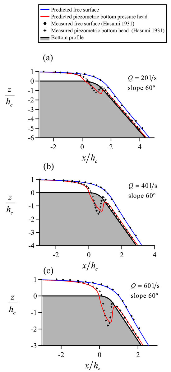
Figure 7.
(a–c) Flow in transition of horizontal channel to 60°: comparison of irrotational flow model with experiments [61]. The scaling used is hc = (q2/g)1/3.
4.3. Flow over the Spillway of a High Dam
In this section, flow over a spillway crest is considered. The geometry for the crest shape adopted corresponds to the USACE 3-circular profile (R = 0.5HD, R = 0.2HD and R = 0.04HD) for the upstream quadrant [58,62,63], and the power equation
for the downstream profile, where HD is the design head and zb is the bed profile elevation. The upstream face is vertical, and the chute angle is 45°. Other proposals for the upstream quadrant are a 2-circular arc profile and elliptical profile [64,65,66]. Knapp [67] and Hager [68,69] proposed continuous bottom profiles for the entire crest to avoid curvature discontinuities, such as those occurring at the apex and at the joins of the circular arcs on the standard USACE profile considered here.
The ogee crest is the most stringent test case for the irrotational flow model, given the strong pressure drop in the upstream quadrant and the displacement of the critical point for the crest apex due to the strong variation of bottom curvature. Flow over an ogee crest for heads H/HD = 0.5, 1, and 1.33 is considered in Figure 8, where free surface experimental data by USACE [63] is included. Simulated free surface and piezometric bottom pressure profiles are also plotted. The simulation with the irrotational flow model was accomplished using ∆x/HD = 0.02 and 20 streamlines for H/HD = 0.5. For the heads H/HD = 1 and 1.33, this mesh was adequate to simulate the flow profile, yet to obtain an accurate piezometric bottom pressure head estimation in the upstream quadrant, ∆x/HD = 0.01 and 80 streamlines had to be used. In the x-ψ mapping, streamlines cannot become vertical, given that their slope ∂y/∂x appears in the Laplacian Equation (8). It implies that, strictly, the upstream face angle of the spillway cannot be 90°. This face was thus simulated as a 2:1 slope (63.5°). Numerical simulations confirmed that it has a weak effect. It was found possible by numerical experimentation to increase the upstream face angle to almost 80°. However, this demanded too high a number of iterations in the SOR solver for an accurate solution. Results of Figure 8 confirm that the approximation adopted is accurate enough. The spillway discharge coefficient emerges as part of the computational solution, e.g.,
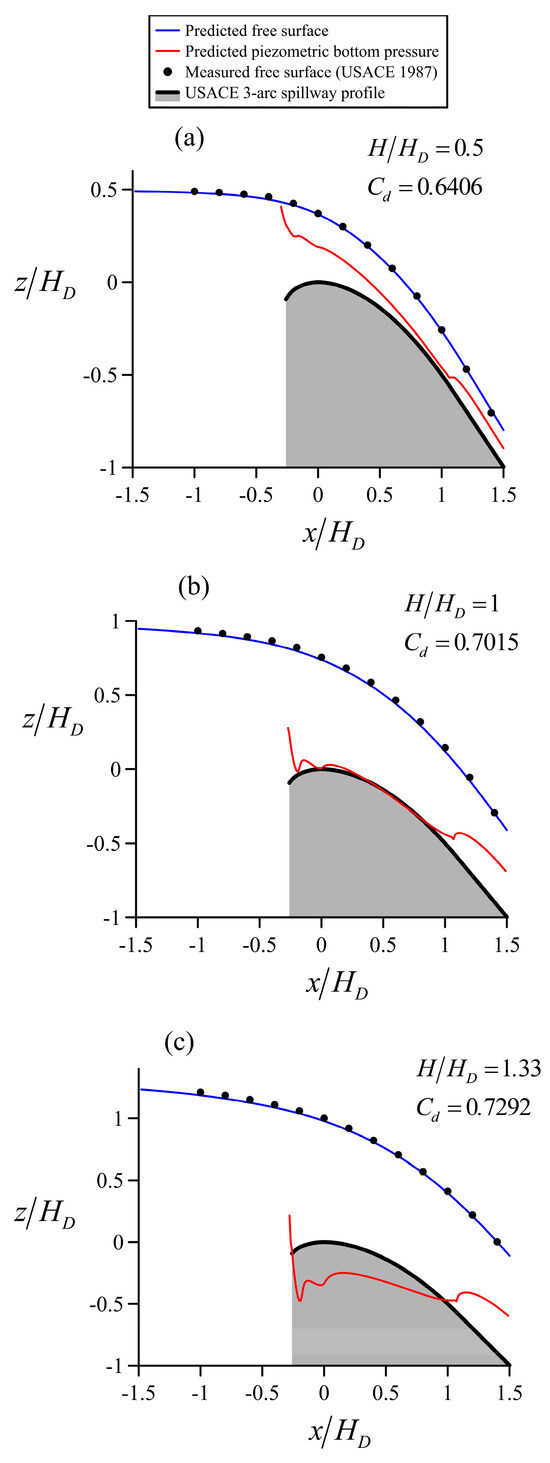
Figure 8.
Flow over an ogee crest for relative heads H/HD = (a) 0.5, (b) 1, and (c) 1.33: comparison with USACE [63] experiments.
Its value is included in Figure 8 for the three runs. It is nearly identical to the experimental values reported by USACE [63]. This is a good advance over former computational models by Cassidy [35], Ikegawa and Washizu [23], or Diersch et al. [22], among others, where the value of Cd was fixed by a trial-and-error procedure observing if the resulting flow profile agreed with observations. Here, both Cd and the flow profile are theoretical results obtained simultaneously without resorting to experimental data.
Comments on the difficulty in obtaining the flow profile in spillway flow follow. Cheng et al. [27] and Liggett [29] used the boundary element method to compute spillway flow. Their model considered a discrete version of Equation (11), which was forced to be satisfied by the free surface each time it was displaced using the Newton–Raphson method. They noted delicate stability problems upstream of the weir crest even when using small corrections to displace the free surface. Lai and Hromadka [70] and Tu [25] had similar problems using the complex variable boundary element method and finite element method, respectively. Montes [16] found that an accurate initial flow profile was needed for convergence, but even in this case, numerical smoothing was needed to stabilize the solution. If Equation (11) is discretized using finite differences, and the Newton–Raphson method used to iterate the free surface position, the same issues were found during this research. On inspecting the resulting algebraical form of Bernoulli’s equation, it was found it had three roots, two of them always positive and nearly identical, complicating the selection of the correct one in a Newton–Raphson code. Further, the method did not yield a physically based estimation of the energy head; thus, incorrect estimations during iterations may produce complex roots and solution failure. In contrast, the proposed method can be used starting the iterations with a rough hydrostatic profile, and the iterative estimation of the energy head ensures that real sub- and supercritical roots are available for all the computational nodes. In addition, the computational load is minimal, only solving the Laplace equation once per surface iteration.
Figure 9 depicts remarkable aspects of the proposed computational method; Figure 9a,c,e show the critical depth profile, minimum total energy head profile, and the critical point for H/HD = 0.5, 1 and 1.33. Note that this is a generalization to 2D irrotational flows of open channel flow concepts used in gradually varied flow computations [32,40]. Second, Figure 9b,d,f present the initial hydrostatic flow profile considered and the final flow profile obtained. Other models for weir flow [16,27,46] demanded a highly accurate initial flow profile to ensure the convergence of a Newton–Raphson-type free surface iteration method. In our case, this was not a limitation, as confirmed by Figure 9. Note the significant displacement of the critical point from the ogee crest in all tests.
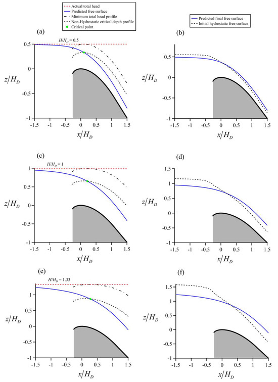
Figure 9.
Flow over an ogee crest for relative heads H/HD = (a) 0.5, (b) 1, and (c) 1.33: determination of the critical point and initial and final free surface profiles.
The bottom pressure head predicted by the irrotational flow model is compared in Figure 10 with data by USACE [63]. The predictions are in fair agreement with the observations, even in the upstream quadrant, where the irrotational model captures the negative pressure peaks correctly.
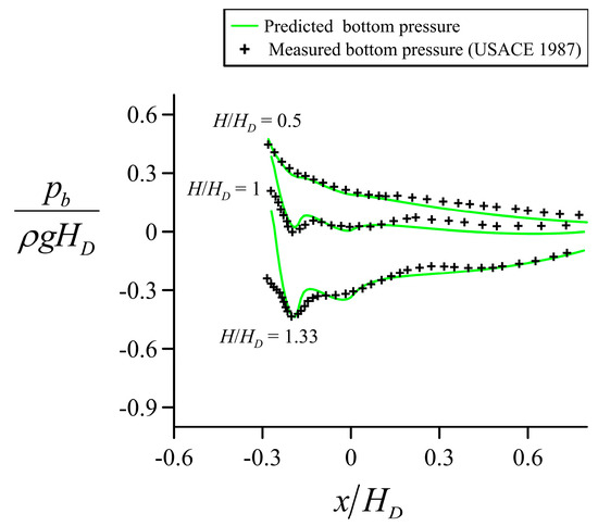
Figure 10.
Flow over an ogee crest for relative heads H/HD = 0.5, 1, and 1.33: comparison of bottom pressure simulations with USACE [63] measurements.
Irrotational model results are compared for heads H/HD equal to 0.5, 1, and 1.33 with CFD results by Ho et al. [71], solving the Navier–Stokes equations using the industrial code in Figure 11. CFD models are an accepted tool to study spillway flow [72]. The irrotational model results are in excellent agreement with CFD results for the free surface, and in close agreement for bottom pressure head simulations.
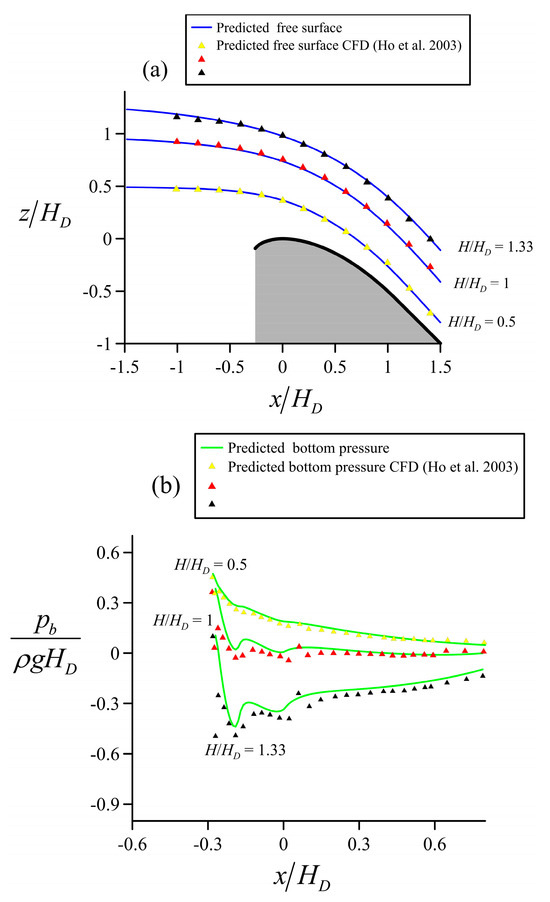
Figure 11.
Flow over an ogee crest for relative heads H/HD = 0.5, 1, and 1.33: comparison of (a) free surface and (b) bottom pressure simulations with CFD results [71].
Model predictions for irrotational crest velocity V for heads H/HD equal to 0.5, 1, and 2 are compared with experimental data by Hager [69] in Figure 12, confirming the accuracy resolving the velocity field of the proposed ideal fluid flow model. The free surface and piezometric bottom pressure head measured by Hager [69] for H/HD = 1 and 2 are considered in Figure 13. The predictions of the irrotational flow model are included there, resulting again in an agreement with the observations. Table 1 contains the Cd experimentally measured by Hager up to the high operational head H/HD ≈ 3. Predicted values of Cd using the irrotational flow solver are included, resulting in small deviations from measurements, in all cases within experimental uncertainty. This confirms that the present model reproduces flow over an ogee crest under a high operational head reasonably well.
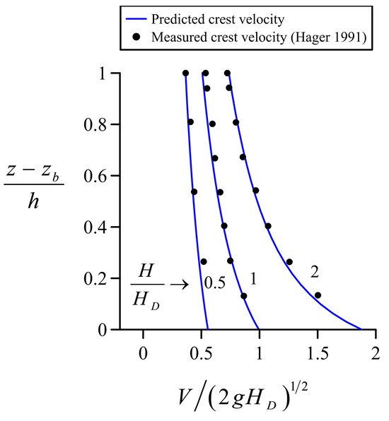
Figure 12.
Comparison of predicted irrotational crest velocity with experimental data [69].
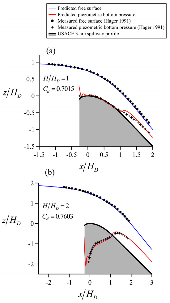
Figure 13.
Flow over an ogee crest for heads H/HD equal to 1 and 2: comparison of (a) free surface and (b) piezometric bottom pressure simulations with Hager’s [69] experiments.

Table 1.
Comparison of predicted Cd(H/HD) by the present irrotational flow model with experimental data for USACE 3-arc spillway by Hager [69]; HD = 0.1 m, chute angle 45°.
5. Discussion of Results
The advantages of the proposed solution method are as follows:
It is not needed to initiate computations with an accurate position of the free surface streamline, e.g., with a Green–Naghdi model, or by resorting to experimental measurements. A hydrostatic flow profile can be settled as a first approximation. This makes the procedure more robust than in other methods.
It is not necessary to form a Jacobian matrix to iterate the free surface position [27], a procedure which would demand to solve the Laplace equation 2N times per surface iteration in our case, with N being the number of nodes in the x-axis. Here, the Laplace equation is solved only once per surface iteration. The computational cost of the method is therefore minimal.
The equations for the free surface movement are analytical and exact; approximations are introduced by the numerically determined α-coefficients. There is no need to use a truncated Taylor series to approximately move the free surface, as in methods based on the Newton–Raphson technique.
The critical point is determined as part of the solution, providing an iterative estimation of the energy head each time the free surface is moved. It is not needed to assume that the critical point is at the weir crest, or use an approximate Taylor expansion to compute the non-hydrostatic critical depth, as that of Jaeger [43,47]. Castro-Orgaz [46], for example, assumed critical flow at a weir crest using Jaeger’s [43] approximate critical flow theory, combined with a Green–Naghdi estimation of the initial water surface. The method worked well for low obstacles, yet failed to produce a solution for spillway flow.
Because the critical point originates as part of the computation [44], the Cd coefficient is automatically determined in the solution procedure. There is no need to use a trial-and-error guessing method as was done by Cassidy [35] or Diersch et al. [22]. Others have used the experimentally obtained Cd, e.g., Montes [16].
Free surface corrections can be large, although we used an average for better convergence. In the Newton–Raphson method, it is mandatory to use minute corrections to obtain real solutions for water depths upstream of the spillway crest. Otherwise, there is a solution failure.
The iteration method used ensures with each free surface movement and new estimated energy head that all free surface roots will be real and positive, eliminating strong stability issues and incorrect root detections originating from directly using the finite difference version of Bernoulli’s equation in the Newton–Raphson method.
The main disadvantage of the proposed method is that the two-branch analytical solution used for free surface determination produces a discontinuous surface curvature hxx when assembling the two portions. This impacts the boundary value problem posed by the Laplace equation, resulting in free surface velocity peaks near the critical point. Those peaks produce α peaks which are transmitted in the form of surface wiggles as water surface iterations progress. However, a simple smoothing filter eliminates the problem.
6. Conclusions
In this work, a method of computing irrotational flow profiles in open channel transitions involving a critical point is proposed. The model entails three ingredients: solution of the Laplacian field using x-ψ mapping, determination of the critical point position and unknown energy head using a critical flow condition for 2D irrotational flows, and analytical determination of the water surface position using exact equations for the sub- and supercritical flow portions.
The method proposed was applied to three relevant cases in practice, namely flow over low obstacles in channels, the transition from mild to steep slopes, and flow over an ogee spillway. In all cases, the simulations for the water surface and piezometric bottom pressure are in reasonable agreement with the observations. For the challenging case of spillway flow, the model results are also in agreement with CFD data. A special feature of the method is that the discharge coefficient emerges as part of the computation, eliminating the need for using trial-and-error techniques as in other methods.
The main advantage of the approach proposed is that the analytical determination of the flow profile uses exact statements combined with a robust estimation of the critical point position. This ensures physically excellent solutions, thereby eliminating the stability and convergence problems present in other methods. The method is simple and clearly related to open channel hydraulics concepts, making it suitable also for teaching purposes.
Author Contributions
Conceptualization, O.C.-O. and W.H.H.; Methodology, O.C.-O.; Software, O.C.-O.; Formal analysis, O.C.-O. and W.H.H.; Investigation, O.C.-O. and W.H.H. All authors have read and agreed to the published version of the manuscript.
Funding
This research received no external funding.
Data Availability Statement
The numerical solver is available from the corresponding author upon reasonable request.
Acknowledgments
The work of O. Castro-Orgaz was supported by the grant María de Maeztu for Centers and Units of Excellence in R&D (Ref. CEX2019-000968-M).
Conflicts of Interest
The authors declare no conflict of interest.
Notation
| u | horizontal velocity |
| w | vertical velocity |
| ψ | stream function |
| z | elevation |
| x | horizontal coordinate |
| V | modulus of velocity vector |
| θ | streamline inclination |
| p | pressure head |
| ρ | water density |
| g | gravity acceleration |
| H | total energy head |
| zs | free surface elevation |
| zb | channel bed elevation |
| E | specific energy |
| Vs | free surface velocity |
| q | discharge per unit channel width |
| α | ratio of surface velocity to depth-averaged velocity |
| hc | critical depth of 2D irrotational flow |
| X, a, b | auxiliar variables |
| Γ | auxiliar function in specific energy |
| i | mesh index |
References
- Castro-Orgaz, O. Steady open channel flows with curved streamlines: The Fawer approach revised. Environ. Fluid Mech. 2010, 10, 297–310. [Google Scholar] [CrossRef]
- Ramamurthy, A.S.; Vo, N.-D.; Balachandar, R. A Note on Irrotational Curvilinear Flow Past a Weir. J. Fluids Eng. 1994, 116, 378–381. [Google Scholar] [CrossRef]
- Rouse, H. The Distribution of Hydraulic Energy in Weir Flow in Relation to Spillway Design. Master’s Thesis, MIT, Boston, MA, USA, 1932. [Google Scholar]
- Rouse, H. Verteilung der Hydraulischen Energie Bei Einem Lotrechten Absturz (Distribution of Hydraulic Energy at a Vertical Drop). Ph.D. Thesis, TU Karlsruhe, Karlsruhe, Germany, 1938. (In Germany). [Google Scholar]
- Rouse, H. Fluid Mechanics for Hydraulic Engineers; McGraw-Hill: New York, NY, USA, 1938. [Google Scholar]
- Hager, W.H. Critical flow condition in open channel hydraulics. Acta Mech. 1985, 54, 157–179. [Google Scholar] [CrossRef]
- Bos, M.G. Discharge Measurement Structures; Intl. Inst. for Land Reclamation (ILRI): Wageningen, The Netherlands, 1976. [Google Scholar]
- Castro-Orgaz, O. Curvilinear flow over round-crested weirs. J. Hydraul. Res. 2008, 46, 543–547. [Google Scholar] [CrossRef]
- Hager, W.H.; Schleiss, A. Constructions Hydrauliques: Ecoulements Stationnaires (Hydraulic Structures: Steady Flows). Traité de Génie Civil 15; Presses Polytechniques Universitaires Romandes: Lausanne, Switzerland, 2009. (In French) [Google Scholar]
- Rouse, H.; Reid, L. Model research on spillway crests. Civ. Engng. 1935, 5, 10–14. [Google Scholar]
- Bettess, P.; Bettess, J.A. Analysis of free surface flows using isoparametric finite elements. Int. J. Numer. Methods Eng. 1983, 19, 1675–1689. [Google Scholar] [CrossRef]
- Thom, A.; Apelt, C. Field Computations in Engineering and Physics; Van Nostrand: London, UK, 1961. [Google Scholar]
- Katopodes, N.D. Free Surface Flow: Computational Methods; Butterworth-Heinemann: Oxford, UK, 2019. [Google Scholar]
- Ganguli, M.K.; Roy, S.K. On the standardisation of the relaxation treatment of systematic pressure computations for overflow spillway discharge. Irrig. Power 1952, 9, 187–204. [Google Scholar]
- Hay, N.; Markland, E. The determination of the discharge over weirs by the electrolytic tank. Proc. Inst. Civ. Eng. 1958, 10, 59–86. [Google Scholar] [CrossRef]
- Montes, J.S. Potential Flow Analysis of Flow Over a Curved Broad Crested Weir. In Proceedings of the 11th Australasian Fluid Mechanics Conference, University of Tasmania, Hobart, Australia, 14–18 December 1992; pp. 1293–1296. [Google Scholar]
- Montes, J.S. Potential-Flow Solution to 2D Transition from Mild to Steep Slope. J. Hydraul. Eng. 1994, 120, 601–621. [Google Scholar] [CrossRef]
- Southwell, R.V.; Vaisey, G. Relaxation methods applied to engineering problems XII. Fluid motions characterized by ‘free’ stream-lines. Philos. Trans. R. Soc. London. Ser. A Math. Phys. Sci. 1946, 240, 117–161. [Google Scholar] [CrossRef][Green Version]
- Barbier, C. Computer Algebra and Transputers Applied to the Finite Element Method. Ph.D. Thesis, Durham University, Durham, UK, 1992. [Google Scholar]
- Betts, P. A variational principle in terms of stream function for free-surface flows and its application to the finite element method. Comput. Fluids 1979, 7, 145–153. [Google Scholar] [CrossRef]
- Dao-Yang, D.; Man-Ling, L. Mathematical Model of Flow Over a Spillway Dam. In Proceedings of the 13th Intl. Congress of Large Dams New Delhi Q50(R55), New Delhi, India, 29 October 1979; pp. 959–976. [Google Scholar]
- Diersch, H.-J.; Schirmer, A.; Busch, K.-F. Analysis of flows with initially unknown discharge. J. Hydraul. Div. 1977, 103, 213–232. [Google Scholar] [CrossRef]
- Ikegawa, M.; Washizu, K. Finite element method applied to analysis of flow over a spillway crest. Int. J. Numer. Methods Eng. 1973, 6, 179–189. [Google Scholar] [CrossRef]
- Nakayama, T.; Ikegawa, M. Finite element analysis of flow over a weir. Comput. Struct. 1984, 19, 129–135. [Google Scholar] [CrossRef]
- Tu, R. Free Boundary Potential Flow Using Finite Elements. Ph.D. Thesis, University of Arizona, Dept. of Civil Engineering and Engineering Mechanics, Tucson, AZ, USA, 1971. [Google Scholar]
- Varoḡlu, E.; Finn, W.L. Variable domain finite element analysis of free surface gravity flow. Comput. Fluids 1978, 6, 103–114. [Google Scholar] [CrossRef]
- Cheng, A.H.-D.; Liu, P.L.-F.; Liggett, J.A. Boundary calculations of sluice and spillway flows. J. Hydraul. Div. 1981, 107, 1163–1178. [Google Scholar] [CrossRef]
- Henderson, H.C.; Kok, M.; De Koning, W.L. Computer-aided spillway design using the boundary element method and non-linear programming. Int. J. Numer. Methods Fluids 1991, 13, 625–641. [Google Scholar] [CrossRef]
- Liggett, J.A. The Boundary Element Method. In Chapter 8, Vol. I of Engineering Applications of Computational Hydraulics; Pitman Publ.: Boston, MA, USA, 1982. [Google Scholar]
- Castro-Orgaz, O.; Hager, W.H. Non-Hydrostatic Free Surface Flows. In Advances in Geophysical and Environmental Mechanics and Mathematics; Springer: Berlin/Heidelberg, Germany, 2017; 696p. [Google Scholar] [CrossRef]
- Castro-Orgaz, O.; Hager, W.H. Shallow Water Hydraulics; Springer: Berlin/Heidelberg, Germany, 2019; 563p. [Google Scholar] [CrossRef]
- Montes, J.S. Hydraulics of Open Channel Flow; ASCE Press: Reston, VA, USA, 1998. [Google Scholar]
- Vallentine, H.R. Applied Hydrodynamics; Butterworths: London, UK, 1969. [Google Scholar]
- Milne-Thomson, L.M. Theoretical Hydrodynamics; MacMillan: London, UK, 1962. [Google Scholar]
- Cassidy, J.J. Irrotational flow over spillways of finite height. J. Eng. Mech. Div. 1965, 91, 155–173. [Google Scholar] [CrossRef]
- Boadway, J.D. Transformation of elliptic partial differential equations for solving two-dimensional boundary value problems in fluid flow. Int. J. Numer. Methods Eng. 1976, 10, 527–533. [Google Scholar] [CrossRef]
- Wilkinson, D.L. Free surface slopes at controls in channel flow. J. Hydraul. Div. 1974, 100, 1107–1117. [Google Scholar] [CrossRef]
- Selby, S.M. Standard Mathematical Tables; CRC: Boca Raton, FL, USA, 1973. [Google Scholar]
- Chanson, H. The Hydraulics of Open Channel Flows: An Introduction; Butterworth-Heinemann: Oxford, UK, 2004. [Google Scholar]
- Chow, V.T. Open Channel Hydraulics; McGraw-Hill: New York, NY, USA, 1959. [Google Scholar]
- Henderson, F.M. Open Channel Flow; MacMillan: New York, NY, USA, 1966. [Google Scholar]
- Fawer, C. Etude de Quelques Écoulements Permanents à Filets Courbes (Study of Some Steady Flows with Curved Streamlines). Ph.D. Thesis, Université de Lausanne, La Concorde, Lausanne, Switzerland, 1937. (In French). [Google Scholar]
- Jaeger, C. Remarques sur quelques écoulements le long des lits à pente variant graduellement (Remarks on some flows along bottoms of gradually varied slope). Schweiz. Bauztg. 1939, 114, 231–234. (In French) [Google Scholar]
- Dao-Yang, D. A numerical method of flow over spillway dam with unknown energy head. Acta Mech. Sin. 1985, 17, 300–308. (In Chinese) [Google Scholar]
- Iwasa, Y. Hydraulic significance of transitional behaviours of flows in channel transitions and controls. Mem. Fac. Eng. Kyoto Univ. 1958, 20, 237–276. [Google Scholar]
- Castro-Orgaz, O. Potential Flow Solution for Open-Channel Flows and Weir-Crest Overflow. J. Irrig. Drain. Eng. 2013, 139, 551–559. [Google Scholar] [CrossRef]
- Jaeger, C. Engineering Fluid Mechanics; Blackie and Son: Edinburgh, UK, 1956. [Google Scholar]
- Sivakumaran, N.S.; Hosking, R.J.; Tingsanchali, T. Steady shallow flow over a spillway. J. Fluid Mech. 1981, 111, 411–420. [Google Scholar] [CrossRef]
- Sivakumaran, N.S.; Tingsanchali, T.; Hosking, R.J. Steady shallow flow over curved beds. J. Fluid Mech. 1983, 128, 469–487. [Google Scholar] [CrossRef]
- Sivakumaran, N.S. Shallow Flow over Curved Beds. Ph.D. Thesis, Asian Institute of Technology, Bangkok, Thailand, 1981. [Google Scholar]
- Castro-Orgaz, O.; Hager, W.H. Curved-streamline transitional flow from mild to steep slopes. J. Hydraul. Res. 2009, 47, 574–584. [Google Scholar] [CrossRef]
- Westernacher, A. Abflussbestimmung an Ausgerundeten Abstürzen mit Fliesswechsel (Discharge Determination at Rounded Drops under Transitional Flow); TU Karlsruhe: Karlsruhe, Germany,, 1965. (In Germany) [Google Scholar]
- Weyermuller, R.G.; Mostafa, M.G. Flow at grade-break from mild to steep slopes. J. Hydraul. Div. 1976, 102, 1439–1448. [Google Scholar] [CrossRef]
- Cassidy, J.J. Designing spillway crests for high-head operation. J. Hydraul. Div. 1970, 96, 745–753. [Google Scholar] [CrossRef]
- Creager, W.P. Engineering for Masonry Dams; Wiley and Sons: New York, NY, USA, 1917. [Google Scholar]
- Escande, L. Détermination pratique du profile optimum d’un barrage déversoir: Tracé des piles par les méthodes aérodynamiques. Application à un ouvrage déterminé (Practical determination of the optimum weir profile: Pier shape using aerodynamic methods, application to prototype structure). Sci. Ind. 1933, 17, 467–474. (In French) [Google Scholar]
- Guo, Y.; Wen, X.; Wu, C.; Fang, D. Numerical modelling of spillway flow with free drop and initially unknown discharge. J. Hydraulic Res. 1998, 36, 785–801. [Google Scholar]
- USACE. Hydraulic Design of Spillways; U.S. Army Corps of Engineers: Washington, DC, USA, 1990. [Google Scholar]
- Ishihara, T.; Iwasa, Y.; Ihda, K. Basic studies on hydraulic performances of overflow spillways and diversion weirs. Bull. Disaster Prev. Res. Inst. 1960, 33, 1–30. [Google Scholar]
- Castro-Orgaz, O.; Cantero-Chinchilla, F.N.; Hager, W.H. High-order shallow water expansions in free surface flows: Application to steady overflow processes. Ocean Eng. 2022, 250, 110717. [Google Scholar] [CrossRef]
- Hasumi, M. Untersuchungen über die Verteilung der hydrostatischen Drücke an Wehrkronen und-Rücken von Überfallwehren infolge des abstürzenden Wassers (Studies on the distribution of hydrostatic pressure distributions at overflows due to water flow). J. Dept. Agric. Kyushu Imp. Univ. 1931, 3, 1–97. (In Germany) [Google Scholar]
- Melsheimer, E.S.; Murphy, T.E. Investigations of Various Shapes of the Upstream Quadrant of the Crest of a High Spillway: Hydraulic Laboratory Investigation; U.S. Army Engineer Waterways Experiment Station: Vicksburg, MS, USA, 1970. [Google Scholar]
- USACE. Hydraulic Design Criteria; U.S. Army Waterways Experiment Station: Vicksburg, MS, USA, 1987. [Google Scholar]
- Maynord, S.T. General Spillway Investigation: Hydraulic Model Investigation; U.S. Army Engineer Waterways Experiment Station: Vicksburg, MS, USA, 1985. [Google Scholar]
- Murphy, T.E. Spillway Crest Design; U.S. Army Engineer Waterways Experiment Station: Vicksburg, MS, USA, 1973. [Google Scholar]
- Reese, A.J.; Maynord, S.T. Design of Spillway Crests. J. Hydraul. Eng. 1987, 113, 476–490. [Google Scholar] [CrossRef]
- Knapp, F.H. Ausfluss, Überfall und Durchfluss im Wasserbau; Braun: Karlsruhe, Germany, 1960. (In Germany) [Google Scholar]
- Hager, W.H. Continuous crest profile for standard spillway. J. Hydraul. Eng. 1987, 113, 1453–1457. [Google Scholar] [CrossRef]
- Hager, W.H. Experiments on standard spillway flow. Proc. ICE 1991, 91, 399–416. [Google Scholar]
- Lai, C.; Hromadka, T.D. Modeling Complex Two-Dimensional Flows by the Complex-Variable Boundary-Element Method. In Proceedings of the Intl. Symp. of Refined Flow Modeling and Turbulence Measurements, Volume II, G-26-1/10, The University of Iowa, Iowa City, IA, USA, 16–18 September 1985. [Google Scholar]
- Ho, D.; Boyes, K.; Donohoo, S.; Cooper, B. Numerical flow analysis for spillways. In Proceedings of the 43rd ANCOLD Conference, Hobart, Tasmania, Australia, 24–29 October 2003. [Google Scholar]
- Savage, B.M.; Johnson, M.C. Flow over ogee spillway: Physical and numerical model case study. J. Hydraul. Eng. 2001, 127, 640–649. [Google Scholar] [CrossRef]


Disclaimer/Publisher’s Note: The statements, opinions and data contained in all publications are solely those of the individual author(s) and contributor(s) and not of MDPI and/or the editor(s). MDPI and/or the editor(s) disclaim responsibility for any injury to people or property resulting from any ideas, methods, instructions or products referred to in the content. |
© 2023 by the authors. Licensee MDPI, Basel, Switzerland. This article is an open access article distributed under the terms and conditions of the Creative Commons Attribution (CC BY) license (https://creativecommons.org/licenses/by/4.0/).