Abstract
Flood disasters are considered to be one of the ten natural disasters that threaten the survival of mankind. They occur frequently and have a serious impact on the national economy. For quicker response to the sudden flood, in this paper, the relevant characteristics of flood forecasting and disaster assessment are comprehensively studied to establish the corresponding models, and a multi-objective culture shuffled complex differential evolution (MOCSCDE) algorithm is proposed to optimize the model parameters. It can achieve better convergence and significantly improve the model accuracy. Then, a river hydrodynamic model is established to simulate the flooding process, and the characteristics of flood evolution, such as water depth, flow speed, duration, and submerged area, are analyzed. Third, based on the above-mentioned flood forecasting and flood evolution calculations, the relative membership function (VFS) is determined via the set pair analysis method (SPA), and the variable fuzzy set model (SPAVFS) is used for flood risk assessment. Finally, through the study of flow forecasting at Zhouqu hydrological station, it is found that the accuracy of the forecast result of the built model is best compared with LSTM and XAJ model, the mean relative error is only 7.6%, and the certainty coefficient can reach 0.96, which surpass the baselines by 20% and 7.9%.
1. Introduction
China, known for its high frequency of flood disasters, is confronted with the serious threat of flash floods that pose a risk to people’s lives and property [1]. To mitigate this risk, accurate flood prediction plays a crucial role in providing timely flood warnings that can save countless lives and protect property. Over the years, extensive research has been conducted on various aspects of flood forecasting, including flood simulation, flood risk assessment, disaster evaluation, and flood control measures [2,3,4]. Among these, flood forecasting has emerged as a widely adopted approach for effective flood control and disaster reduction [5]. Furthermore, significant advancements have been made in the theory and technology of flood forecasting [2].
Hydrological model is the basis of flood forecasting, and it is also an important tool to simulate the hydrological process of the basin. The development of hydrological models can be traced back to the reasoning formula method proposed by Mulvaney in 1851. In the 1950 s, with the rapid development of computer, 3S, and other technologies, hydrological models, represented by watershed hydrological models, flourished, such as the Standford model, HBV model, Shanbei model, SWAT model, VIC model, and so on. They have been applied to flood forecasting and have achieved good flood control and disaster reduction effects.
Ye et al. [6] utilized the Xin’anjiang model to develop a program for flash flood forecasting in small and medium rivers located in humid regions. Zhang et al. [7] applied the HEC-HMS model to a small watershed in the Loess Plateau, while Liu et al. [8] implemented the LL-II distributed model. Additionally, Li et al. [9] enhanced the capabilities of the CASC2D model. Moreover, several distributed forecasting models have produced significant research findings. For example, Javier et al. [10] integrated geographic information system (GIS), radar rainfall estimation, and other cutting-edge technologies to establish a flood forecasting and early warning system for small watersheds. As for flood simulation methods, the traditional methods mostly come from engineering hydrology calculation methods; for instance, the API (preliminary rainfall index) rainfall–runoff empirical correlation method is used more for runoff generation, and the Sherman unit line is used more for confluence [11]. The effect of these methods is influenced by the limitation of calculation conditions, and they had the characteristics of simple calculation and strong practicability [12]. Later, with the rapid development of computing technology, hydrological model methods became the mainstream of flood simulation and were widely used because of higher forecasting accuracy and more comprehensive functions after more practice tests and screenings of flood simulation methods [3,13,14].
Hydrological model parameters play a crucial role in the forecasting performance of hydrological models [15,16]. Because of the nonlinearity of the hydrological model and the characteristics of the model parameters, such as high latitude, multiple constraints, and incomplete independence, the optimization of hydrological model parameters has always been a key and difficult point in the field of hydrological research [17]. Traditional hydrological model parameter optimization methods include the artificial experience method and trial-and-error method [18,19,20], which mainly rely on the experience of hydrologists to adjust the model parameters and constantly try to calculate and compare them until obtaining satisfactory results. This type of method is highly subjective, computationally intensive, and time-consuming. With the development of computers and other technologies, there are a variety of computer-based parameter optimization methods, widely used genetic algorithms, particle swarm algorithms, SCE-UA algorithms [18,21,22]. However, based on a single objective function of the hydrological model parameter optimization method, we cannot fully explore the hydrological model, which contains a variety of information characteristics, so the direction of parameter optimization has changed gradually from single-objective optimization to multi-objective optimization. Deb et al. [23] proposed a second-generation dominance ranking algorithm, Zitzler [24] pro-posed the SPEA-2 algorithm based on the Pareto dominance relation, and Guo et al. [25] proposed a multi-objective hybrid complex-form difference evolutionary algorithm. The multi-objective culture shuffled complex differential evolution (MOCSCDE) is used to optimize the parameters of the prediction model. The algorithm has better global convergence and can effectively reduce the uncertainty of model parameters. Thus, it can greatly improve the prediction accuracy of the model [26].
In practical engineering applications, increasing the accuracy of flood prediction is an essential project to research urgently. In this paper, a model of northern Shaanxi suitable for arid and semi-arid areas in Zhouqu County, Gansu Province, was established, and the parameters of the hydrological model were optimized via the MOCSCDE multi-objective optimization calibration method. The improved northern Shaanxi-MOCSCDE forecasting method was applied to the flash flood forecasting in Zhouqu County, and the forecasting results were compared with the Xin’anjiang model and the LSTM model. The results show that the improved northern Shaanxi-MOCSCDE forecasting method has the best forecasting effect.
In recent years, there has been a growing interest among researchers in the application of convolutional neural networks (CNN) for time series forecasting [27]. Irena Koprinska et al. proposed a CNN-based model for energy time series prediction, which consisted of two convolution layers and two fully connected layers. In a similar vein, Mikolaj Binkowski et al. [28] introduced an autoregressive convolutional neural network specifically designed for asynchronous time series. This model utilized two separate convolutional neural networks to process the input time series. Furthermore, Fu et al. [29] developed an innovative unsupervised deep neural network known as the sequential update reconstruction with time series memory autoencoder (SUR-TSMAE). This model allows for the direct input of multidimensional time series data and simultaneously extracts features from both the feature dimension and the time dimension.
2. Flood Control Simulation and Dispatching System
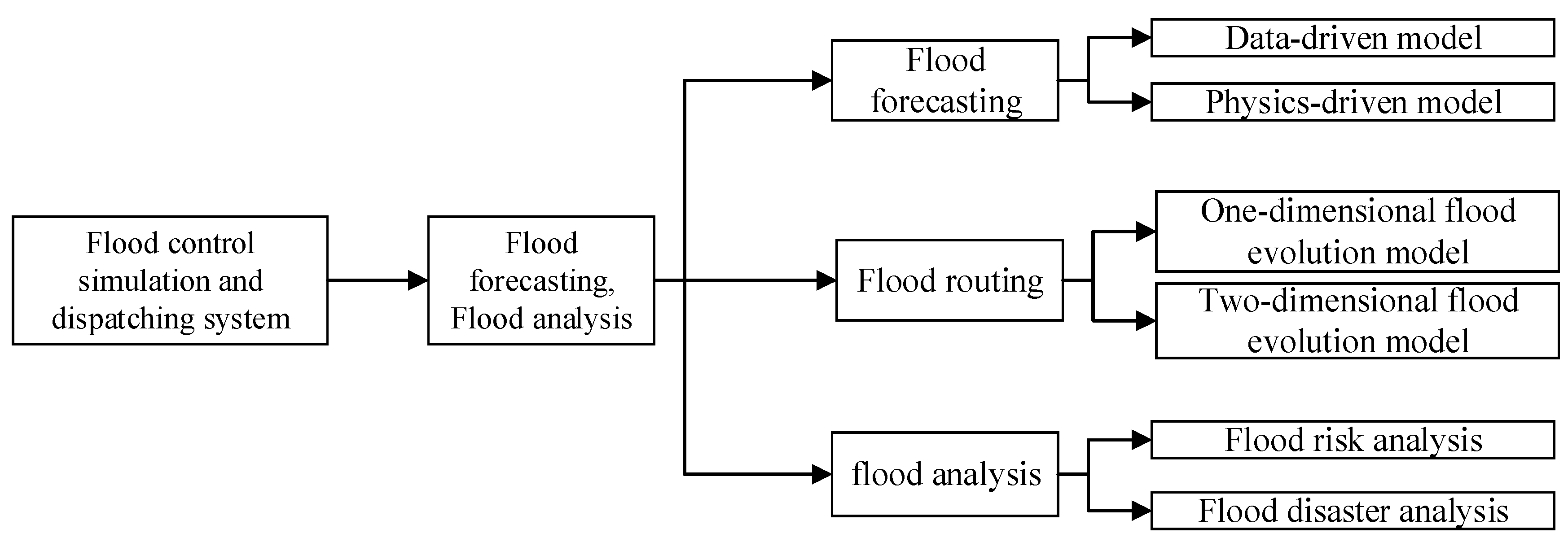
This paper establishes a system for flood simulation and dispatching, which includes essential functions such as the home page, basic information management and maintenance, and system management and maintenance. The system consists of core functional modules, namely, flood forecasting, flood evolution, flood risk analysis, and flood three-dimensional display, as depicted in Figure 1. In the flood forecasting module, we employ a combination of data-driven models and physical-driven models, which include LSTM, SVM, and other data-driven models, as well as northern Shaanxi models, API models, and other physical-driven models.
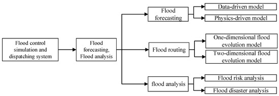
Figure 1.
Functional structure diagram of flood control dispatching system.
The flood evolution module incorporates both the commonly used one-dimensional river simulation model and a newly developed two-dimensional hydrodynamic model. In particular, the new 2D model introduces a novel formulation for conserving the classical two-dimensional shallow water equations. This model accurately depicts flood conditions such as water depth and velocity. For the flood risk analysis module, we have developed flood risk assessment and flood disaster estimation. The flood risk assessment module integrates the fuzzy comprehensive assessment method, variable fuzzy sets theory, attribute interval identification theory, and other methods. Notably, this paper proposes a comprehensive flood risk assessment approach named SPAVFS. In the flood disaster estimation module, we have constructed a flood disaster evaluation model that considers the loss rate database, social–economic spatial distribution database, and inundation analysis database.
3. Flood Forecasting Method Based on MOCSCDE
As the research subject is situated in the arid inland area of northwest China, it falls under the category of super-permeable runoff with minimal snowmelt runoff during the flood season. In this context, the Shanbei model, which represents the rainfall runoff in Shanbei, can serve as the appropriate runoff generation model suitable for arid and semi-arid regions. The Shanbei model offers numerous advantages, including a rational structure and straightforward calculations.
3.1. Model Theory
To account for the heterogeneity of rainfall and the distribution of underlying surfaces, particularly the unevenness of ground infiltration capacity, the practical application of the Shanbei model involves dividing the watershed into multiple units. Each unit consists of an impermeable area FB and a permeable area (1 − FB). In the impermeable area, the runoff R2 is generated by subtracting the evapotranspiration E from the rainfall P. In the permeable area, the runoff R2 is calculated using the Horton infiltration formula and the distribution curve of drainage capacity after deducting the evapotranspiration E from the rainfall. The total runoff for the basin is obtained as R = R1 + R2. The slope confluence of each unit area is computed using either a linear reservoir or a lag algorithm, while the river confluence is computed using the Muskingen piecewise continuous algorithm. The principle of the Shanbei model is illustrated in Figure 2.
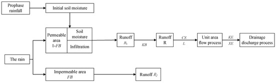
Figure 2.
Workflow of rainfall-runoff in Shanbei model.
3.2. Model Parameters and Calibration Method
When the Horton infiltration formula is applied to the runoff calculation of the Shanbei model, the parameters KC, θm, FB, f0, fc, K, B, CS, L are included.
(1) Evapotranspiration reduction factor KC:
KC is the ratio of the evapotranspiration capacity of the basin to the measured value of the surface evaporator and is the most important parameter affecting the calculation of flow yield. Due to the data of arid areas and other reasons, the KC value often varies greatly in the actual simulation calculation, which must be determined after debugging and can be selected by month if necessary. The value ranges from 0.5 to 1.0.
(2) Tension water storage capacity θm:
Together with parameter KC, it is mainly used to calculate the initial soil water content θ0, generally θm = 60~80 mm.
(3) Watershed impermeability ratio FB:
Parameter FB reflects the proportion of impermeable area in the whole watershed.
(4) The ability of infiltration during the most drought f0:
Generally, there is no soil moisture content and infiltration data in the natural watershed, which can be analyzed by hydrologic analysis and infiltration model method and verified by measured data, generally f0 = 1.0~2.0 mm/min.
(5) Stable infiltration rate fc:
The principle is the same as f0, generally fc = 0.3~0.5 mm/min.
(6) Holden infiltration curve equation coefficient K:
The principle is the same as f0, generally K = 0.04~0.05/min.
(7) Infiltration capacity distribution curve parameter B:
Parameter B reflects the distribution characteristics of infiltration capacity on the permeable area, and B = 0 indicates that the infiltration capacity is evenly distributed. The larger B is, the more uneven the distribution of infiltration rate is. The value of B depends on the soil structure of the basin.
(8) Surface runoff settlement coefficient CS:
CS stands for tempering effect. Since the rate of retreat is generally related to the flow of retreated water, it can be analyzed by the flow of retreated water.
(9) Confluence lag L:
The lag time L generally varies with the size of the flood. If the confluence of large floods is fast, L will be small; if the confluence of small floods is low, L will be large.
In consideration of the traditional single-objective hydrological model cannot accurately assess all the behaviors within the system. In order to forecast floods more accurately, in this article, an efficient evolution algorithm entitled MOCSCDE is proposed to improve the model parameters. It has good convergence and diffusivity on multiple objectives, and greatly improves the model accuracy. These forecasting results can be used to study the dam break mechanism.
It is assumed that optimization is carried out in a multi-objective framework. If there are conflicts between the pre-defined target functions, then the final results cannot be one individual but a group of individuals, which are collectively referred to as non-dominated results. If the ultimate goal of all objective functions is to achieve minimization, the optimization problem is as follows:
where M is the number of objective functions, X stands for the model parameters, and fi is the i-th objective function. The objective functions are as follows:
where N is the sample length, Qi denotes the i-th observed value, and is the i-th forecasting value. In the process of solving the above objectives by the MOCSCDE algorithm, the parameters that need to be customized are mainly as follows:
Population size, N; dimensions of decision variables, D; target space dimension O; crossover probability, CR; the number of complex words in situational knowledge (SK), NC; evolutionary algebra before complex mixing, NBS; algorithm maximum evolution algebra, Max; the size of the set of non-inferior individuals PiC (i = 1, 2, …, NC) obtained by each complex search in SK, NPC; the size of the set of non-inferior individuals P obtained by the whole population optimization calculation in SK, NP; evolutionary interval NM generations of history knowledge, HK; among these, HK is used to record the process of algorithm evolution calculation. In this paper, HK is used to preserve the degree of difference between individuals in the population P and to determine whether to use the Cauchy variation threshold ε or Cauchy’s coefficient of variation η.
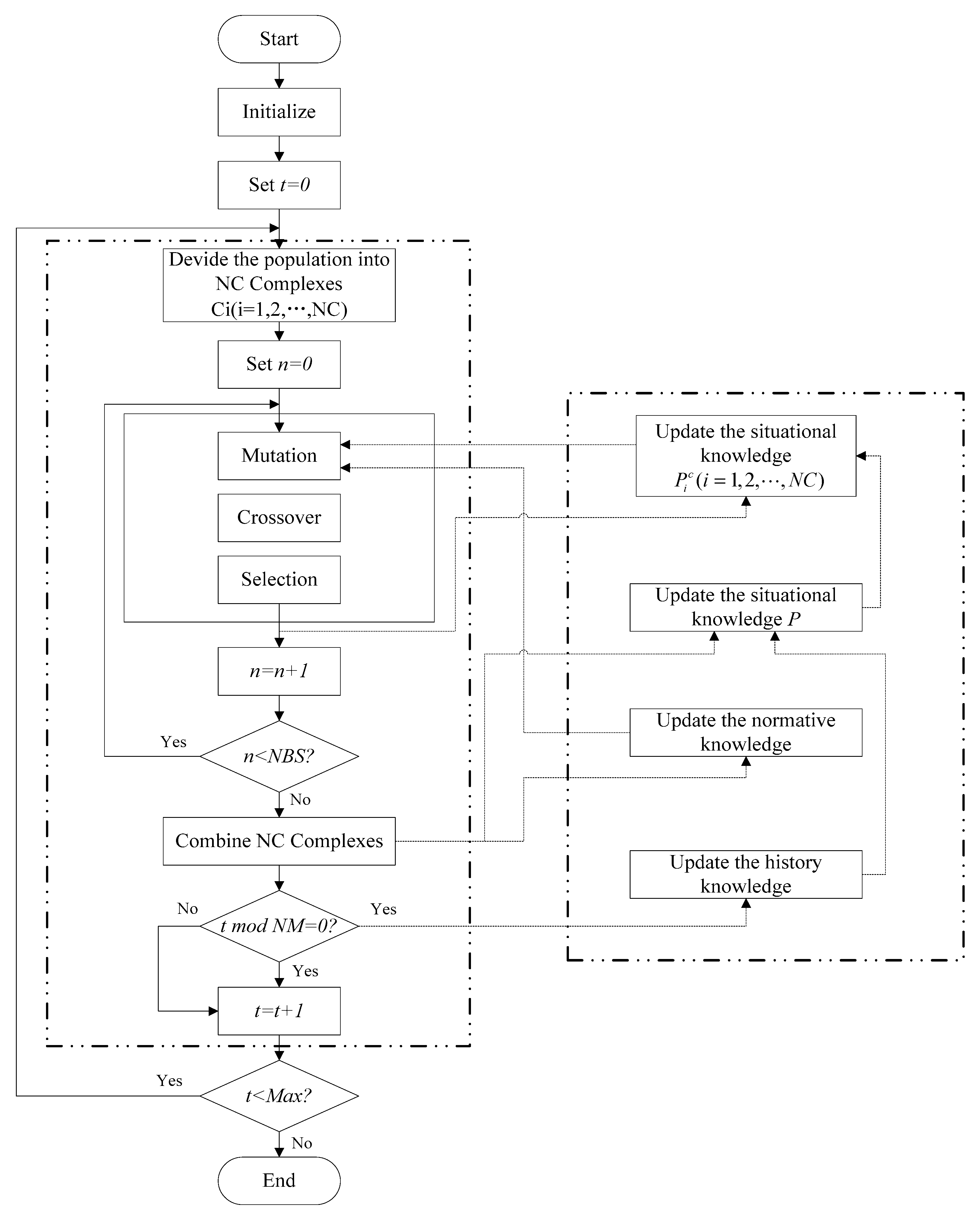
The calculation steps of the MOCSCDE algorithm are described as follows:
Step 1: Initialize the (population space) PS and generate (belief space) BS by extracting knowledge information according to PS;
Step 2: According to Pareto ranking results of individual groups, the groups can be divided into NC Complexes;
Step 3: The evolutionary calculus of variation, crossover, selection, and so on is carried out for each Complex separately and based on (Situational Knowledge) SK during evolution, (Normative Knowledge) NK, and (History Knowledge) HK to guide. Every evolutionary computation generation, update the PiC (i = 1, 2, …, NC).
Step 4: After each Complex evolves NBS generation, mix all Complexes, and update P and NK in SK;
Step 5: Update HK after every evolution NM generation;
Step 6: Determine whether the maximum evolutionary algebra Max is reached; if not, jump to Step 2; if so, jump to Step 7;
Step 7: The evolution is over, and the calculation result is output.
The flowchart of the MOCSCDE is shown in Figure 3.

Figure 3.
Flowchart of the MOCSCDE algorithm.
4. Flood Risk and Disaster Estimation
4.1. Flood Risk Estimation
The estimation of flood risk entails a comprehensive assessment that considers numerous factors [30,31]. Due to the intricate interplay of natural, social, and economic factors in each region, there lacks a standardized quantitative criterion for certain aspects. Consequently, the flood risk assessment index system becomes complex, making it challenging to conduct the assessment [32]. To overcome these obstacles and adhere to the principles of being systematic, quantitative, operable, and universal, we have established a first-level evaluation index system for flood risk in flood diversion areas, drawing on the theory of the disaster system. Through local surveys, historical references, and other means, we have developed scoring criteria for each factor.
In this study, we propose and apply a novel flood risk comprehensive assessment method called the set pair analysis-variable fuzzy sets model (SPAVFS) based on set pair analysis (SPA) and variable fuzzy set (VFS) theory. The SPAVFS model exhibits advantages in terms of intuitive stability and enhanced universality.
4.2. Flood Disaster Estimation
The first part of the model consists of many databases. After comprehensive consideration of the three factors, the flood disaster assessment model can be expressed as follows:
where i, j, and k are the cell codes of the computational grid, the land use type, and water depth, respectively. Aij represents the original related social–economic unit value of the jth disaster-affected body of the ith computing unit. ηjk represents the loss rate, which is the combination of the j-type disaster-affected-body and the k-level water depth. αi represents the state of the computational grid. When i = 1, it means that we pay attention to the land use type to compute the loss; when i = 0, it indicates that the land use type of the region is other.
The concrete steps of the grid-based flood analysis model are as follows:
(1) The results of the 2D hydrodynamic model are used to record the water depth and the flow velocity of the nodes; then, the flood inundation grid is obtained by the GIS spatial analyst component and IDW (inverse distance weighted) interpolation method.
(2) A series of GIS tools are developed to process raster data. All the flood evolution grids are reclassified to six levels of water depth and blended with the land-use raster.
(3) Grid-based disaster estimation models, based on GIS raster computation and depth-duration-damage equations, are used to generate the flood evolution raster and add up the submerge data by time sequence. In addition, the models can punish integrated flood disaster maps with the GIS platform.
5. Experiment
5.1. Study Area
Our research area is located in Zhouqu County, Gansu Province, China, between 104°07′30′′ E and 105°30′30′′ E longitude, and 33°20′ to 34°34′ N latitude. The county stretches 99.4 km from east to west and 88.8 km from north to south, with a total area of 3009.98 km2. The terrain slopes high from the northwest to the southeast, featuring a landscape of overlapping mountains, gorges, and rugged terrain. Zhouqu County is situated in the Jialing River Basin within the South Qinling Mountains, characterized by a typical high mountain and canyon topography, with steep slopes, deep valleys, sparse vegetation, and severe soil erosion.
The average annual temperature in Zhouqu County is 12 °C, with extreme highs reaching 38.2 °C and extreme lows dropping to −10.2 °C. The average annual precipitation is 700 mm, with a coefficient of variation of 0.2. The majority of rainfall occurs between May and September, accounting for 80.4% of the annual precipitation. The average annual evaporation is 1975.2 mm. The relative humidity stands at 65%. The average annual wind speed is 2.1 m/s, with the maximum wind speed reaching 12 m/s. The maximum snow depth is 7 cm, and the annual sunshine duration is 1929.9 h. The maximum depth of frozen soil reaches 24 cm.
5.2. Experimental Settings
5.2.1. Datasets
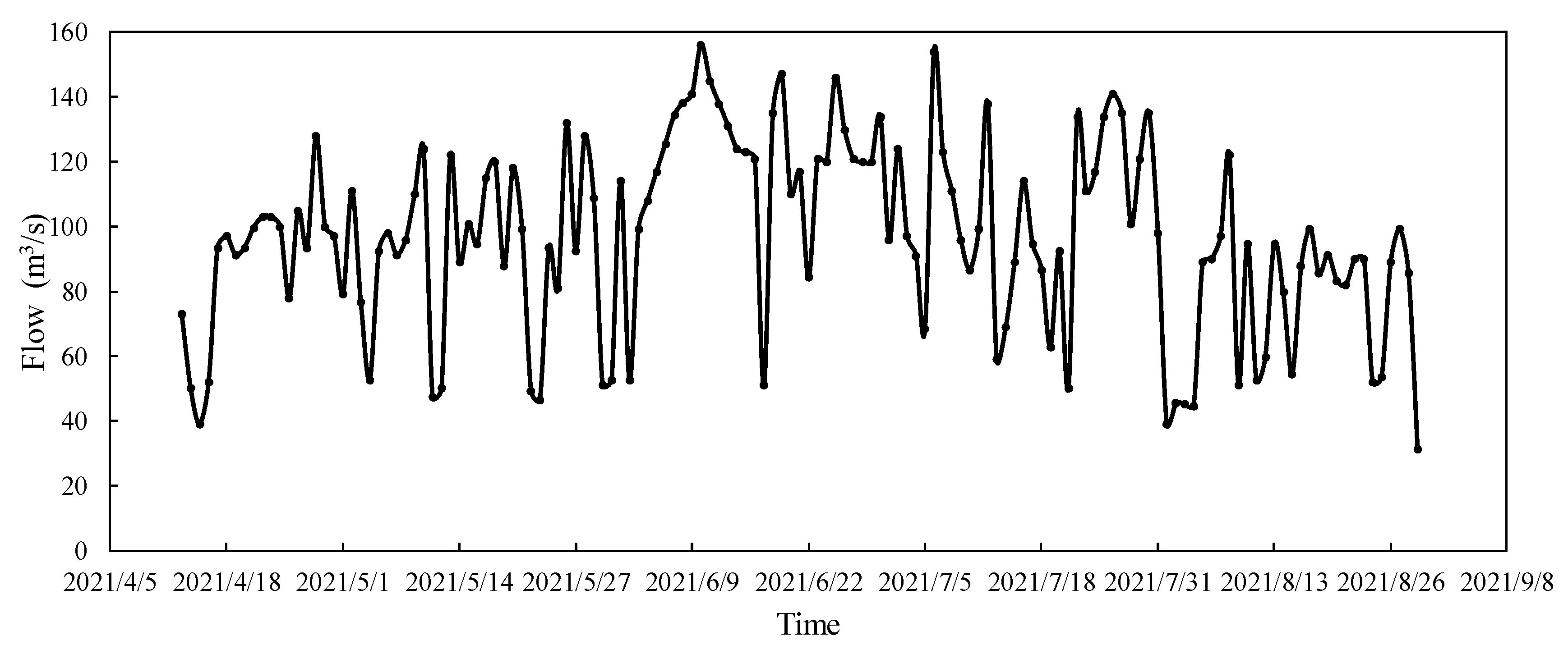
To gain further insights into the prediction capabilities of the MOCSCDE flood forecasting model, we applied the Shanbei model to simulate the runoff of the Zhouqu hydrological station based on its historical data. Due to data limitations, the model primarily incorporates the daily flow data and corresponding rainfall data spanning approximately 510 days from 23 March 2020 to 9 August 2021. The first 3/4 of the dataset was utilized for model calibration, while the remaining 1/4 was used for verification purposes. Although the hydrological data are derived from a single observed station, the improved prediction model’s applicability extends to other watersheds.
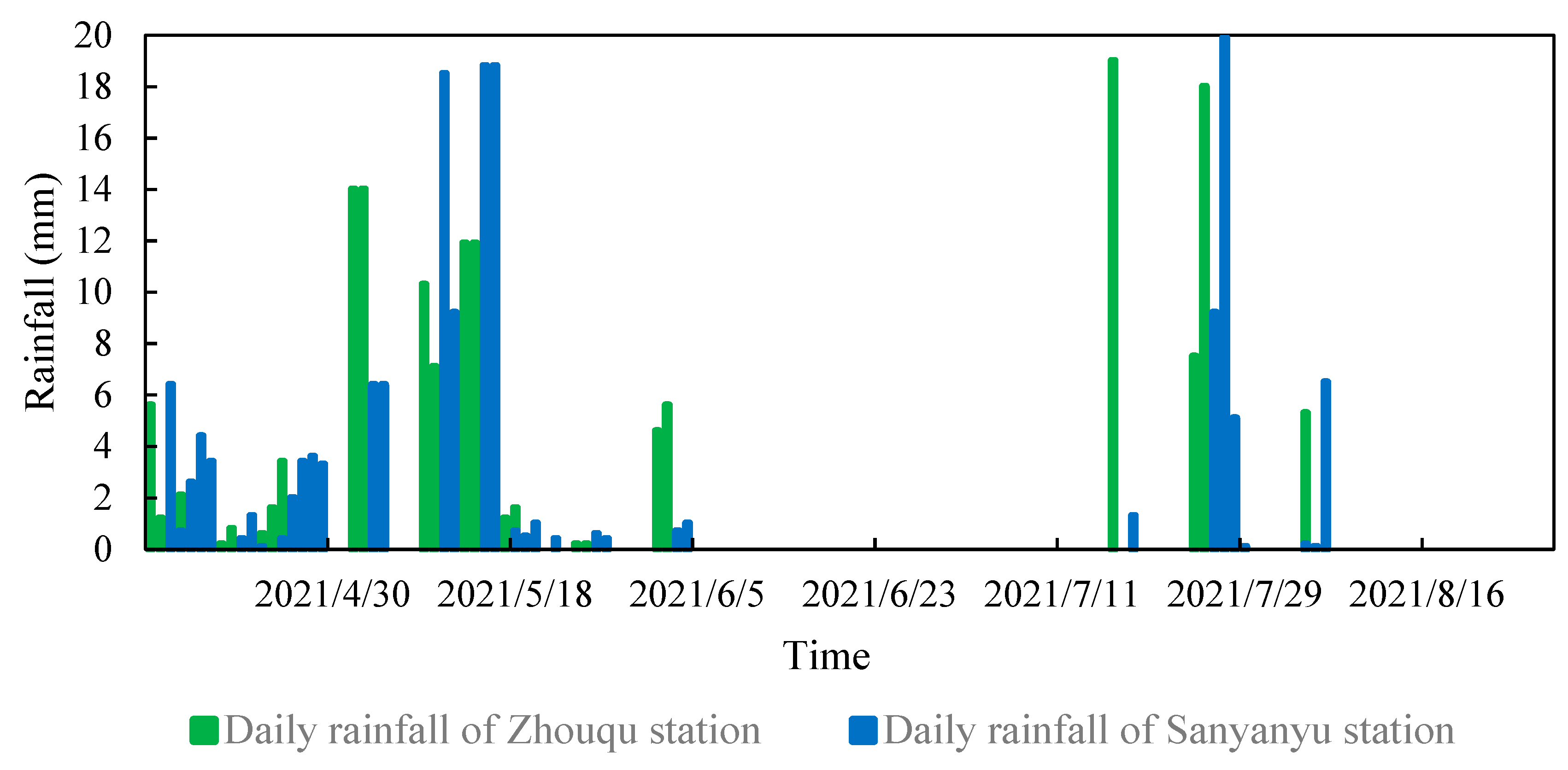
Figure 4 presents the measured daily flow data of the Zhouqu hydrological station, while Figure 5 showcases the corresponding rainfall data from both the Zhouqu and Sanyanyu stations.
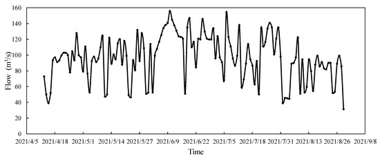
Figure 4.
Measured daily flow data of Zhouqu hydrological stations.
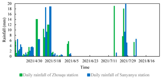
Figure 5.
The corresponding rainfall data of Zhouqu and Sanyanyu station.
For comparison purposes, this study utilizes the LSTM model [33,34] and the XAJ model to predict the flow of hydrological stations in Zhouqu using the same historical flow data. The LSTM model is a commonly employed data-driven model known for its high computational accuracy and stability. Hence, we choose this method as a baseline to evaluate our proposed approach. LSTM is a time loop neural network that leverages long-term effective short-term memory to preserve states along the time axis (referred to as cell state). This state is not only passed to the subsequent time step but also remains effective for an extended duration [35]. Within the LSTM node, special processes are performed by incorporating three ‘gates’—i.e, the ‘forgetting gate,’ the ‘input gate,’ and the ‘output gate’—to receive information generated by the previous node.
The XAJ model, proposed by Professor Zhao Renjun, is a lumped hydrological model specifically designed for inflow and runoff forecasting for the XAJ Reservoir [36]. One notable feature of this model is its division into three components: units, water sources, and stages. Sub-unit division involves the partitioning of the entire basin into multiple units to consider uneven rainfall distribution and facilitate consideration of variations in underlying surface conditions. Water source separation entails dividing the runoff into three components: surface, soil, and underground [37]. These three water sources possess varying confluence velocities, with the surface having the fastest and the underground the slowest. The stage division is based on different characteristics during the confluence process, with the slope confluence stage and the river network confluence stage treated separately. In the slope stage, different water sources have varying confluence velocities, while such differences are not present in the river network.
5.2.2. Evaluation Metrics
After the runoff prediction model is established and is used to obtain the runoff forecast, it is necessary to evaluate the forecast effect and analyze the accuracy and practicability of the runoff forecast results. The model performance evaluation mainly uses the following accuracy indicators.
(1) Mean absolute error (MAE):
It represents the absolute difference between the predicted value and the true value. The formula is as follows:
where n represents the number of prediction results, yi represents the true value, and represents the predicted value.
(2) Mean relative error (MRE):
It represents the relative gap between the predicted value and the true value. The formula is as follows:
The meaning of each variable in the formula is the same as Formula (5).
(3) Coefficient of certainty (R2):
The degree of fit reflects the degree of fit of the predicted result to the trend of the true result. The formula is as follows:
where represents the average value of the actual results, and the meaning of the remaining variables is the same as Formula (5)
5.2.3. Implementation Details
The implementation details mainly include the following steps:
Step 1: Data collection and processing include rainfall data collection, processing of typical rainfall stations, and collection and processing of historical runoff data from hydrological stations;
Step 2: Based on the historical rainfall and runoff data, the Shanbei model is established, and the parameter rate and model verification calculation are carried out, including runoff generation calculation and tributary confluence calculation based on the Muskingen method;
Step 3: Based on the topographic data of the main channel, a two-dimensional hydrodynamic model is constructed. The tributary flow obtained in Step 2 is used as the input of the model to obtain the flow process of the section of Zhouqu hydrological station;
Step 4: Using the historical flow process, the LSTM model is used as the baseline, the model is built to obtain the forecast runoff series under comparative conditions.
Step 5: Comparing the calculation results of the method proposed with the calculation results of the LSTM model, the rationality and validity of the proposed method are analyzed.
5.3. Results and Discussion
For the Shanbei model, after many experiments, it is found that the sensitivity parameters of the Shanbei model include KC, θm, K, and CS. the parameters before and after model optimization are shown in Table 1, the statistical indicators of the simulation results of the Shanbei model before and after the parameter optimization are shown in Table 2.

Table 1.
Optimized model parameters reference values with MOCSCDE.
Table 2.
The statistical indicators of the simulation results of Shanbei model before and after parameter optimization.
It can be seen from Table 1 that the parameters after optimization are different from those before optimization. Among them, KC, θm,, and K show a decreasing trend, and CS shows an upward trend. The remaining parameter values remain unchanged.
It can be seen from Table 2 that the forecast results calculated by applying the aforementioned hydrological model are generally good. After the parameter optimization, the MAE is reduced from the initial 6.16 to 5.16, a decrease of 1.0, and the reduction rate is 16.23%. The MRE decreases from the initial 8.62% to 7.60%, a decrease of 1.2, and the reduction rate is 11.83%. The R2 increases from 0.9 to 0.96 at the beginning, an increase of 0.06, and the increase rate is 6.67%.
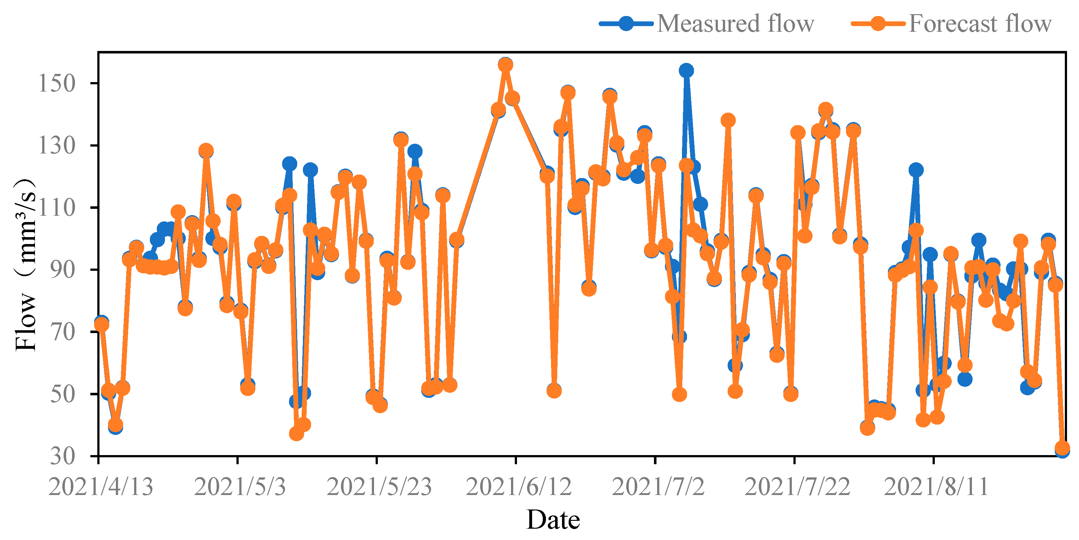
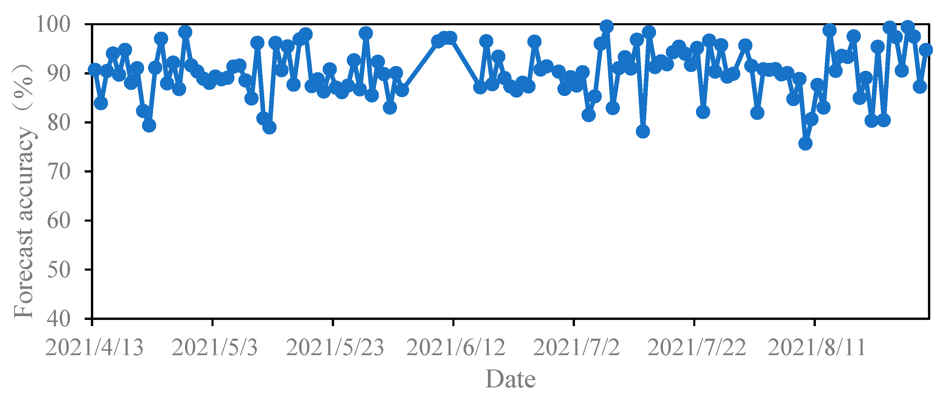
In addition, the comparison chart of the forecast flow process, the scatter plot of the forecast result, and the forecast accuracy change graph in the verification period are shown in Figure 6, Figure 7 and Figure 8, respectively.
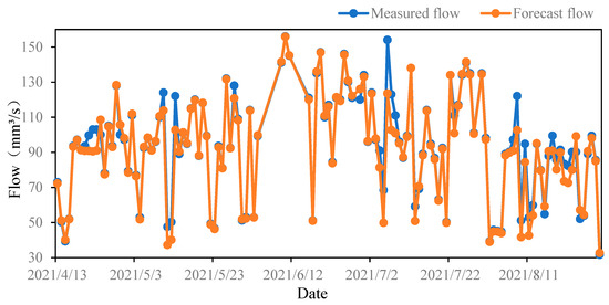
Figure 6.
Comparison diagram of forecast runoff process of Shanbei model.
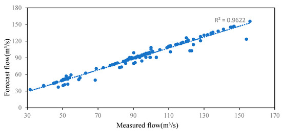
Figure 7.
Scatter plot of forecast results of Shanbei model.
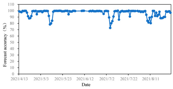
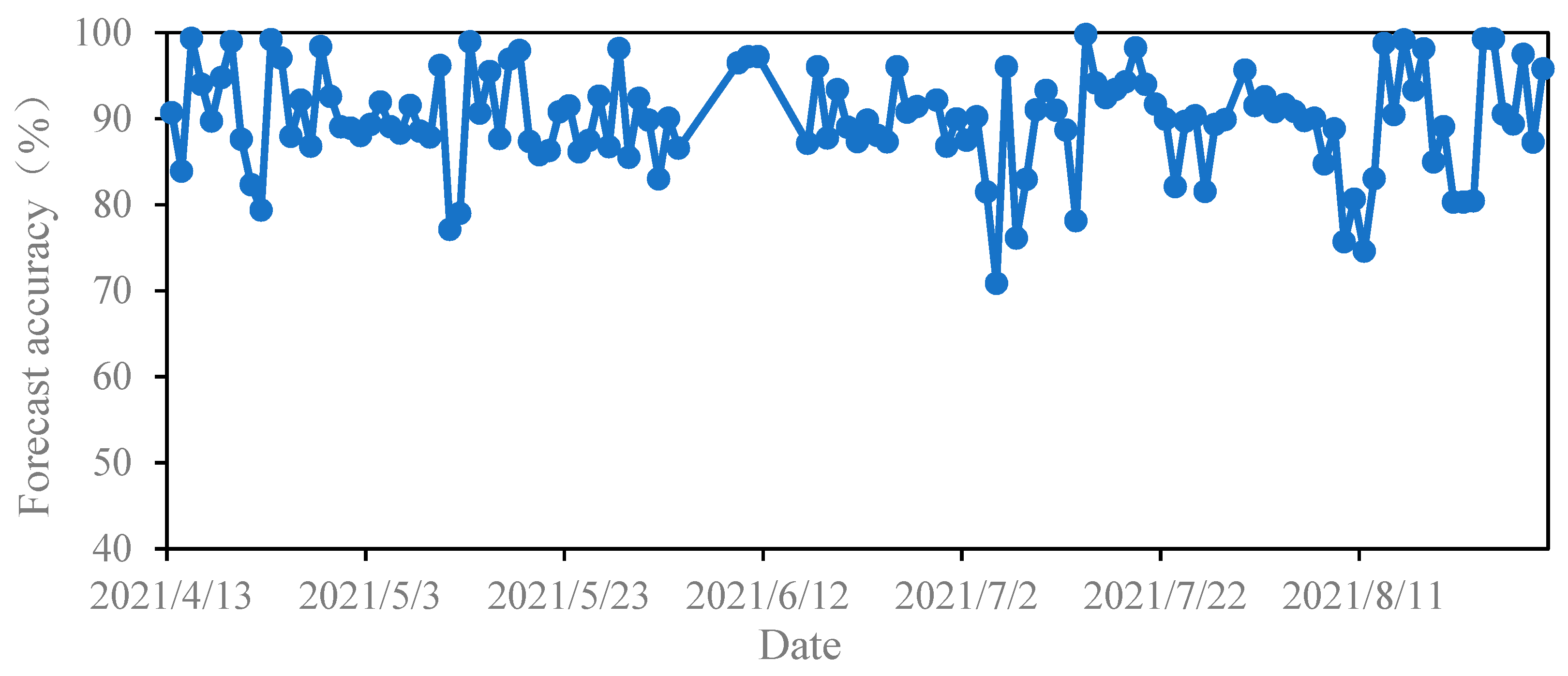
Figure 8.
Forecast accuracy change map of Shanbei model.
It can be seen from Figure 6, Figure 7 and Figure 8 that the change trends of measured runoff and forecast runoff are relatively consistent. The overall process has a good fitting effect except for individual extreme points. In most cases, the forecast accuracy is above 90%, and the forecast accuracy is high, which meets the requirements of practical applications.
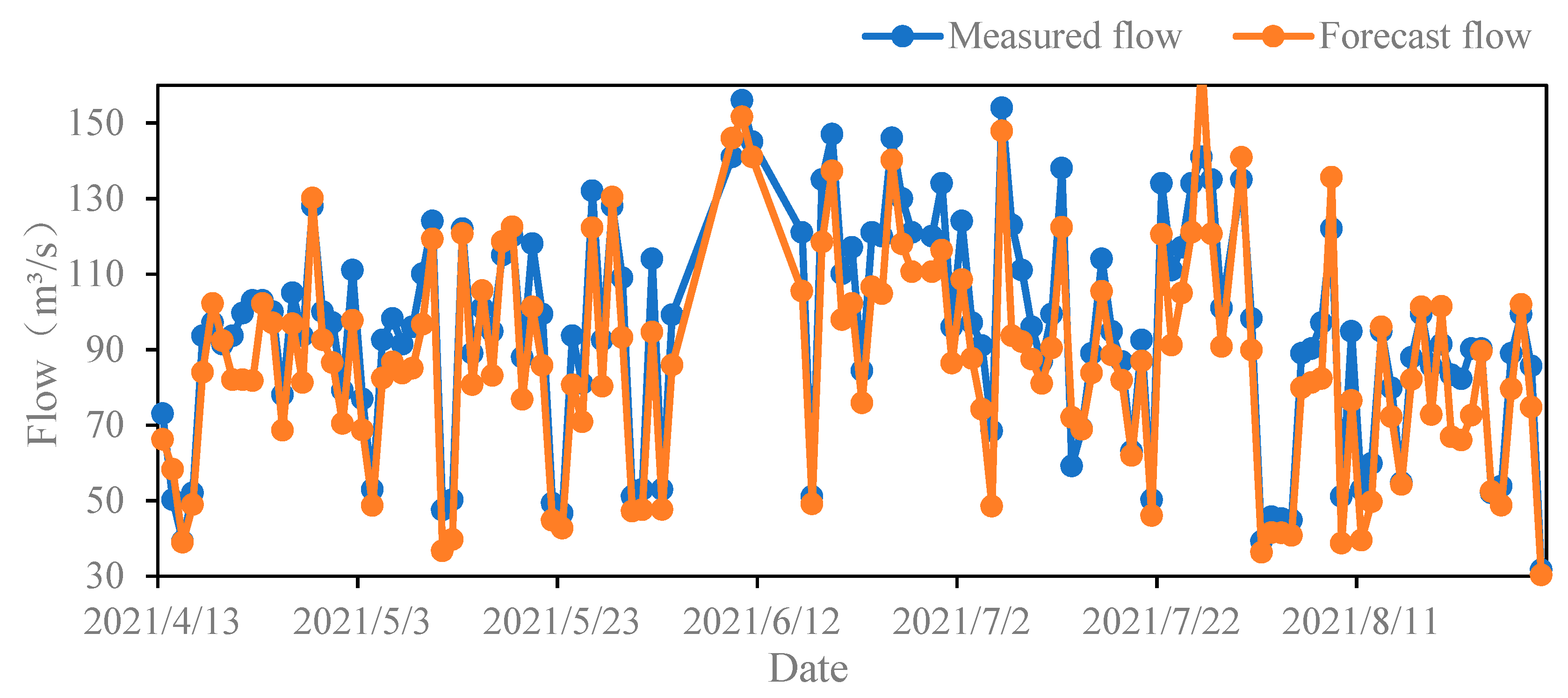
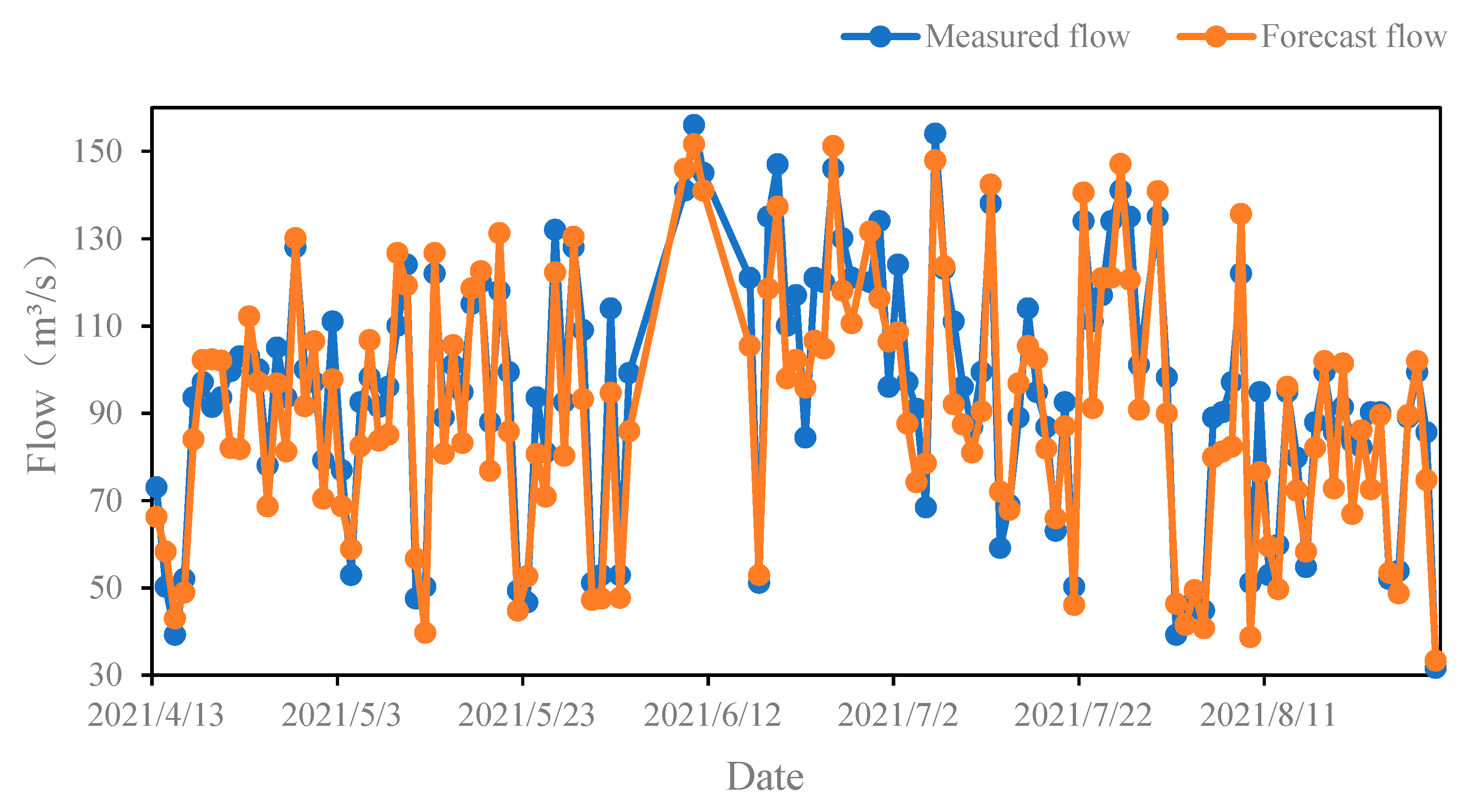
As a comparison, the obtained statistical indicators of the simulation results by the LSTM model and XAJ model are shown in Table 3. For the XAJ model, the comparison chart of the forecast runoff process, the scatter plot of forecast result, and the forecast accuracy change graph are shown in Figure 9, Figure 10 and Figure 11, respectively. For the LSTM model, the comparison chart of the forecast runoff process, the scatter plot of forecast result, and the forecast accuracy change graph are shown in Figure 12, Figure 13 and Figure 14, respectively.
Table 3.
The statistical indicators of the simulation results of the LSTM and XAJ model.

Figure 9.
Comparison diagram of forecast runoff process of the XAJ model.
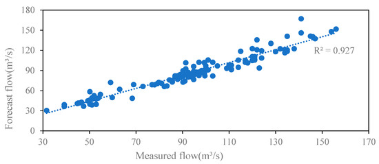
Figure 10.
Scatter plot of forecast results of the XAJ model.
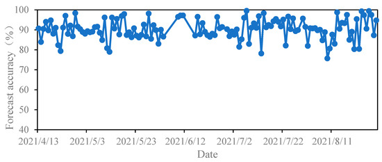
Figure 11.
Forecast accuracy change graph of the XAJ model.
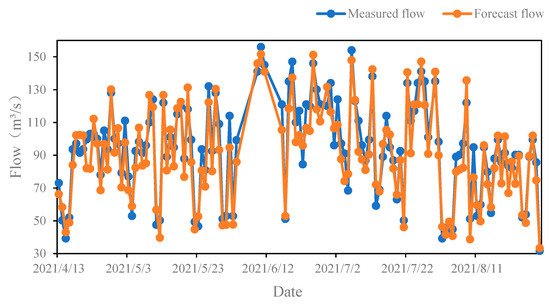
Figure 12.
Comparison diagram of forecast runoff process of LSTM model.
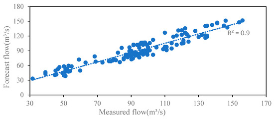
Figure 13.
Scatter plot of forecast results of LSTM model.
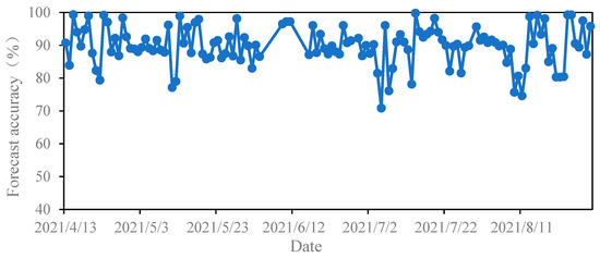
Figure 14.
Forecast accuracy change graph of LSTM model.
From Table 3, it can be seen that although the MRE of the data-driven model LSTM can be controlled within 10% with high accuracy, the result is worse than that of the proposed model in this paper, it has increased by 25.00%. Moreover, the MAE increases from 5.16 in the proposed model to 10.26 in LSTM model, and the R2 decreases from 0.96 in Shanbei model to 0.89 in the LSTM model, decreasing by 7.29%. For the XAJ model, the MRE has increased by 13.16%. Moreover, the MAE increases from 5.16 in the proposed model to 6.03 in the XAJ model, and the R2 decreases from 0.96 in Shanbei model to 0.90 in LSTM model, decreasing by 6.67%.
It can be seen from Figure 9, Figure 10 and Figure 11 that the change trends of measured runoff and forecast runoff are relatively consistent. However, the fit is poor at the peak of the flow. In most cases, the forecast accuracy is above 88%, and the forecast accuracy is 0.90. On the whole, the effect is lower than that of the Shanbei model.
It can be seen from Figure 12, Figure 13 and Figure 14 that the change trends of measured runoff and forecast runoff are relatively consistent. However, the fit is also poor at the peak of the flow. In most cases, the forecast accuracy is above 85%, and the forecast accuracy is 0.89, which is lower than that of the Shanbei and XAJ models.
On the whole, it can be seen from Figure 6, Figure 7, Figure 8, Figure 9, Figure 10, Figure 11, Figure 12, Figure 13 and Figure 14 that compared with the other two models, the change trends of measured runoff and forecast runoff in the Shanbei model are more consistent, the value of R2 is the largest, and the prediction accuracy is also the highest, which indicates that the Shanbei model has the best prediction effect. The main reason is that the Shanbei model is a physically driven model, which can simulate the physical process of rainfall and flow well and has high accuracy in application in small watersheds. For the XAJ model, it is a lumped hydrological model, which can generalize the hydrological process of the basin or the transformation process of rain and flood into several key links such as runoff and confluence [38]. The model has few parameters, and the calibration is relatively easy. After the model parameters are verified, the prediction accuracy is high, but it cannot describe the spatial variation information of the hydrological physical process. As for the LSTM model, it is the data-driven model, which completely depends on the accuracy of historical data and has low accuracy when there is a certain amount of data error or insufficient data.
6. Conclusions
This study initially examines the key characteristics of flood forecasting, flood simulation, flood risk, and disaster assessment. Based on this foundation, we developed a flood prediction model that integrates rainfall generation, confluence, and river course evolution, using the Shanbei model and a river hydrodynamic model. To optimize the parameters of the forecast model, we proposed a novel approach that employs the MOCSCDE algorithm.
Through a case study on inflow forecasting for the Zhouqu hydrological station, we find that our proposed model achieves a mean relative error (MRE) of only 7.6 and an R2 value of 0.96. In comparison, the XAJ model and LSTM model exhibit lower prediction accuracy evaluation metrics when compared to the optimized model. Our optimized model excels in simulating flood forecasts for Zhouqu, demonstrating remarkable performance. This achievement is highly commendable for the flood prevention department as it provides them with a reliable and precise prediction model. The main limitation of this study lies in the outdated theoretical mechanism of the model, as it is not the most recent flood forecasting model based on the latest theories. However, considering the circumstances of our research area, it was not feasible to use data-driven forecasting models with their required input and calibration conditions. Therefore, we employed the simple yet innovative SHANBEI model coupled with the MOCSCDE algorithm, which yielded satisfactory flood forecasting results. We consider this research outcome to hold significant importance for the study area, despite the limitation that our research approach cannot be directly applied in well-documented and moist basins.
In conclusion, the innovative approach of employing multiple models for flood forecasting, simulation, and evaluation proposed in this study holds great significance for decision-makers in formulating proactive adaptive measures. It offers superior performance and empowers decision-makers to take proactive actions.
Author Contributions
Y.L. (Yongfeng Li): Conceptualization, Methodology, Visualization, Data curation, Writing—Original draft preparation, Writing—Review and editing. Y.L. (Yi Liu): Writing the introduction, Visualization. X.L.: Validation, Software, Supervision. C.S.: Visualization, Investigation, Resources. All authors have read and agreed to the published version of the manuscript.
Funding
This study was financially supported by the National Key R&D Program of the 14th Five-Year Plan(2022YFC3002704); the Natural Science Foundation of China (52179016); and the General project of Hubei Provincial Natural Science Foundation (2022CFB042).
Data Availability Statement
Some or all data, models, or code that support the findings of this study are available from the corresponding author upon reasonable request.
Acknowledgments
The authors are grateful to the anonymous reviewers for their comments and valuable suggestions.
Conflicts of Interest
The authors have no conflict of interest to declare.
References
- Che, H.; Wang, J. Sparse Nonnegative Matrix Factorization Based on Collaborative Neurodynamic Optimization. In Proceedings of the 2019 9th International Conference on Information Science and Technology (ICIST), Hulunbuir, China, 2–5 August 2019; pp. 114–121. [Google Scholar]
- Xu, Y.; Wang, X.; Jiang, Z.; Liu, Y.; Zhang, L.; Li, Y. An Improved Fineness Flood Risk Analysis Method Based on Digital Terrain Acquisition. Water Resour. Manag. 2023, 37, 3973–3998. [Google Scholar] [CrossRef]
- Xu, Y.; Jiang, Z.; Liu, Y.; Zhang, L.; Yang, J.; Shu, H. An Adaptive Ensemble Framework for Flood Forecasting and Its Application in a Small Watershed Using Distinct Rainfall Interpolation Methods. Water Resour. Manag. 2023, 37, 2195–2219. [Google Scholar] [CrossRef]
- Burstein, O.; Grodek, T.; Enzel, Y.; Helman, D. SatVITS-Flood: Satellite Vegetation Index Time Series Flood Detection Model for Hyperarid Regions. Water Resour. Res. 2023, 59, e2023WR035164. [Google Scholar] [CrossRef]
- Guo-wei, L. Definition and classification of non-structure measures for flood prevention. Adv. Water Sci. 2003, 14, 98. [Google Scholar]
- Ye, J.; Wu, Y.; Li, Z.; Chang, L. Research and application of small and medium-sized flash flood forecasting methods in humid regions. Hehai Univ. Sci. (Ed.) 2012, 40, 615–621. [Google Scholar]
- Zhang, J.; Na, L.; Zhang, B. Applicability of the distributed hydrological model of HEC-HMS in a small watershed of the Loess Plateau area. J. Beijing For. Univ. 2009, 31, 52–57. [Google Scholar]
- Liu, Z.; Li, L.; Zhu, C.; Wu, J.; Dai, R. Comparative study of distributed hydrological models in flood forecasting. Hydropower Energy Sci. 2006, 2, 70–73. [Google Scholar]
- Li, Z.; Hu, W.; Ding, J.; Hu, Y.; Wu, Y.; Li, J. Research on distributed hydrological model based on physical foundation and grid. J. Hydroelectr. Power 2012, 2, 5–13. [Google Scholar]
- Javier, J.R.N.; Smith, J.A.; Meierdiercks, K.L.; Baeck, M.L.; Miller, A. Flash flood forecasting for small urban watersheds in the Baltimore metropolitan region. Weather. Forecast. 2007, 22, 1331–1344. [Google Scholar] [CrossRef]
- Karpatne, A.; Ebert-Uphoff, I.; Ravela, S.; Babaie, H.A.; Kumar, V. Machine Learning for the Geosciences: Challenges and Opportunities. IEEE Trans. Knowl. Data Eng. 2019, 31, 1544–1554. [Google Scholar] [CrossRef]
- Sainju, A.M.; He, W.; Jiang, Z. A Hidden Markov Contour Tree Model for Spatial Structured Prediction. IEEE Trans. Knowl. Data Eng. 2022, 34, 1530–1543. [Google Scholar] [CrossRef]
- Singh Vijay, P.; Woolhiser David, A. Mathematical Modeling of Watershed Hydrology. J. Hydrol. Eng. 2002, 7, 270–292. [Google Scholar] [CrossRef]
- Sahoo, R.; Zhao, S.; Chen, A.; Ermon, S. Reliable decisions with threshold calibration. Adv. Neural Inf. Process. Syst. 2021, 34, 1831–1844. [Google Scholar]
- Shen, Y.; Wang, S.; Zhang, B.; Zhu, J. Development of a stochastic hydrological modeling system for improving ensemble streamflow prediction. J. Hydrol. 2022, 608, 127683. [Google Scholar] [CrossRef]
- Chilkoti, V.; Bolisetti, T.; Balachandar, R. Investigating the role of hydrological model parameter uncertainties in future streamflow projections. J. Hydrol. Eng. 2020, 25, 05020035. [Google Scholar] [CrossRef]
- Eidsvik, J.; Mukerji, T.; Bhattacharjya, D. Value of Information in the Earth Sciences: Integrating Spatial Modeling and Decision Analysis; Cambridge University Press: Cambridge, UK, 2015. [Google Scholar]
- Zhang, X.; Srinivasan, R.; Zhao, K.; Liew, M. Evaluation of global optimization algorithms for parameter calibration of a computationally intensive hydrologic model. Hydrol. Process. 2009, 23, 430–441. [Google Scholar] [CrossRef]
- Arsenault, R.; Poulin, A.; Côté, P.; Brissette, F. Comparison of stochastic optimization algorithms in hydrological model calibration. J. Hydrol. Eng. 2014, 19, 1374–1384. [Google Scholar] [CrossRef]
- Huo, J.; Liu, L.; Zhang, Y. Comparative research of optimization algorithms for parameters calibration of watershed hydrological model. J. Comput. Methods Sci. Eng. 2016, 16, 653–669. [Google Scholar] [CrossRef]
- Chu, W.; Gao, X.; Sorooshian, S. A solution to the crucial problem of population degeneration in high-dimensional evolutionary optimization. IEEE Syst. J. 2011, 5, 362–373. [Google Scholar] [CrossRef]
- Chen, Y.; Li, J.; Xu, H. Improving flood forecasting capability of physically based distributed hydrological models by parameter optimization. Hydrol. Earth Syst. Sci. 2016, 20, 375–392. [Google Scholar] [CrossRef]
- Deb, K.; Agrawal, S.; Pratap, A.; Meyarivan, T. A fast elitist non-dominated sorting genetic algorithm for multi-objective optimization: NSGA-II. In Parallel Problem Solving from Nature-PPSN VI, Proceedings of the 6th International Conference, Paris, France, 18-20 September 2000; Springer: Berlin/Heidelberg, Germany, 2000; pp. 849–858. [Google Scholar]
- Guo, J.; Zhou, J.; Zou, Q.; Liu, Y.; Song, L. A novel multi-objective shuffled complex differential evolution algorithm with application to hydrological model parameter optimization. Water Resour. Manag. 2013, 27, 2923–2946. [Google Scholar] [CrossRef]
- Zitzler, E.; Laumanns, M.; Thiele, L. SPEA2: Improving the Strength Pareto Evolutionary Algorithm; ETH Zurich, Computer Engineering and Networks Laboratory: Zurich, Switzerland, 2001; Volume 103. [Google Scholar]
- Li, C.; Han, Z.; Li, Y.; Li, M.; Wang, W.; Dou, J.; Xu, L.; Chen, G. Physical information-fused deep learning model ensembled with a subregion-specific sampling method for predicting flood dynamics. J. Hydrol. 2023, 620, 129465. [Google Scholar] [CrossRef]
- Zhang, M.; Ding, D.; Pan, X.; Yang, M. Enhancing Time Series Predictors With Generalized Extreme Value Loss. IEEE Trans. Knowl. Data Eng. 2023, 35, 1473–1487. [Google Scholar] [CrossRef]
- Binkowski, M.; Marti, G.; Donnat, P. Autoregressive convolutional neural networks for asynchronous time series. In Proceedings of the International Conference on Machine Learning, Stockholm, Sweden, 10–15 July 2018; pp. 580–589. [Google Scholar]
- Fu, S.; Zhong, S.; Lin, L.; Zhao, M. A Novel Time-Series Memory Auto-Encoder With Sequentially Updated Reconstructions for Remaining Useful Life Prediction. IEEE Trans. Neural Netw. Learn. Syst. 2022, 33, 7114–7125. [Google Scholar] [CrossRef]
- Kang, S.; Yin, J.; Gu, L.; Yang, Y.; Liu, D.; Slater, L. Observation-Constrained Projection of Flood Risks and Socioeconomic Exposure in China. Earth’s Future 2023, 11, e2022EF003308. [Google Scholar] [CrossRef]
- Awasthi, C.; Archfield, S.A.; Reich, B.J.; Sankarasubramanian, A. Beyond Simple Trend Tests: Detecting Significant Changes in Design-Flood Quantiles. Geophys. Res. Lett. 2023, 50, e2023GL103438. [Google Scholar] [CrossRef]
- Shi, P.; Du Juan, J.M.; Liu, J.; Wang, J. Urban risk assessment research of major natural disasters in China. Adv. Earth Sci. 2006, 21, 170. [Google Scholar]
- Altan, A.; Karasu, S.; Zio, E. A new hybrid model for wind speed forecasting combining long short-term memory neural network, decomposition methods and grey wolf optimizer. Appl. Soft Comput. 2021, 100, 106996. [Google Scholar] [CrossRef]
- Mohamed, T.; Sayed, S.; Salah, A.; Houssein, E.H. Long Short-Term Memory Neural Networks for RNA Viruses Mutations Prediction. Math. Probl. Eng. 2021, 2021, 9980347. [Google Scholar] [CrossRef]
- Sherstinsky, A. Fundamentals of Recurrent Neural Network (RNN) and Long Short-Term Memory (LSTM) network. Phys. D Nonlinear Phenom. 2020, 404, 132306. [Google Scholar] [CrossRef]
- Wang, J.; Bao, W.; Gao, Q.; Si, W.; Sun, Y. Coupling the Xinanjiang model and wavelet-based random forests method for improved daily streamflow simulation. J. Hydroinformatics 2021, 23, 589–604. [Google Scholar] [CrossRef]
- Wu, Y.; Xu, W.; Yu, Q.; Feng, J.; Lu, T. Hierarchical Bayesian Network Based Incremental Model for Flood Prediction. In MultiMedia Modeling, Proceedings of the 25th International Conference, MMM 2019, Thessaloniki, Greece, 8–11 January 2019; Springer: Cham, Switzerland, 2019; pp. 556–566. [Google Scholar]
- Zhou, Y.; Wu, Z.; Xu, H.; Wang, H.; Ma, B.; Lv, H. Integrated dynamic framework for predicting urban flooding and providing early warning. J. Hydrol. 2023, 618, 129205. [Google Scholar] [CrossRef]


Disclaimer/Publisher’s Note: The statements, opinions and data contained in all publications are solely those of the individual author(s) and contributor(s) and not of MDPI and/or the editor(s). MDPI and/or the editor(s) disclaim responsibility for any injury to people or property resulting from any ideas, methods, instructions or products referred to in the content. |
© 2023 by the authors. Licensee MDPI, Basel, Switzerland. This article is an open access article distributed under the terms and conditions of the Creative Commons Attribution (CC BY) license (https://creativecommons.org/licenses/by/4.0/).