1. Introduction
Water is one of the essential components of life; without water there is no existing life possible on the earth. Despite that 66% of the total earth is made up of water, out of this, only 1% of water is usable, and the rest is not safe to use because either it is saltwater or saline. From an economic point of view, water is an important part of a nation’s economy and wealth. However, during the last few years, water levels have fallen considerably, and this comes as one of the biggest emerging problems of today’s world [
1]. As the world population keeps increasing and the predicted growth of the population puts water resources under pressure, providing clean water to this growing population has become a challenging task. The rapid growth of the population is a threatening situation that directly affects the water quality (WQ) as well, and the cost to provide safe water is increasing rapidly [
2]. According to research, the lack of clean water might increase the probability of individuals living in poverty. Water distribution is uneven between countries. The accessible amount of water is 60% [
3], which means that water is easily available to use and abundant on Earth; it is accessible for industry, agriculture, and for drinking use [
4].
Rivers and groundwater are the fundamental sources of fresh water; social and economic development is directly linked with fresh water [
5]. Due to human activities, both surface water and groundwater are under great pressure. Activities such a commercialization, urbanization, population growth, and industrialization have a direct impact on water quality and quantity [
6]. Additionally, climate change and global warming have a worse effect on water quality. Therefore, water quality evaluation and estimation are of great concern today [
7].
The index used for the assessment and classification of surface water and groundwater is the water-quality index (WQI). WQI is a widely used parameter for water-quality classification. For water-quality level estimation, Brown et al. [
8] proposed an index. The index is computed based on water physiochemical parameters such as pH, the concentration of pollutants, dissolved oxygen, temperature, turbidity, and biochemical oxygen demand. For policymakers, this WQI parameter gives meaningful qualitative data and is helpful for the planners of water distribution systems. The drawback of WQI is that it consists of lengthy and complex computations, and a lot of time and effort are needed in this regard [
9]. To address the above-mentioned problems, it is the need of the hour to have an alternative and state-of-the-art system for efficient water-quality classification (WQC).
AI-based modeling removes the complex and lengthy calculations and classifies WQI promptly [
9]. Therefore, water-quality classification using an artificial intelligence-based system is getting the attention of many researchers. Different researchers have proposed different WQC systems using machine learning and deep learning models. Predominantly, such efforts often achieve low accuracy. Furthermore, the available dataset for the experiments has some missing values that are much-needed for water-quality prediction and have a direct impact on the results.
Clean and easily available water is required for drinking, home usage, recreational activities, and food production. Better water-supply and resource management may significantly increase a country’s economic development. Sufficient water should be available for personal and domestic usage and should always be safe, easily accessible, and available to everyone. Every year, many individuals die from kidney failure, cancer, and other diseases caused by polluted water. Laboratory methods for classifying water quality are resource-intensive and time-consuming. Many water-quality classification methods are already available; however, many lack accuracy. As a result, it is very important to have an automated system that can classify water quality with low human effort and with time efficiency.
The continuous, diligent evaluation and acceptability of drinking water sources by the public health community is referred to as potable-water-quality surveillance. A perfect water distribution and monitoring system guarantees people’s health if the potable water is treated without errors. Further, the perfect water treatment system is in vain if the architecture of the water supply and water treatment allows contamination into the potable water. During the last decade, concerns about water contamination have been raised. Prediction of water quality comes out as an important topic as it directly relates to life survival on earth. As a result, there is a vast amount of work on automated water-quality prediction techniques. Such efforts often yield comparably low accuracy. Moreover, the dataset available for experimentation had missing values and missing attributes. These missing values affect the results of water-quality prediction. To address this issue efficiently, this study made the following contributions
A novel HO AutoML stacked ensemble model is proposed that provides higher accuracy for drinking water-quality prediction.
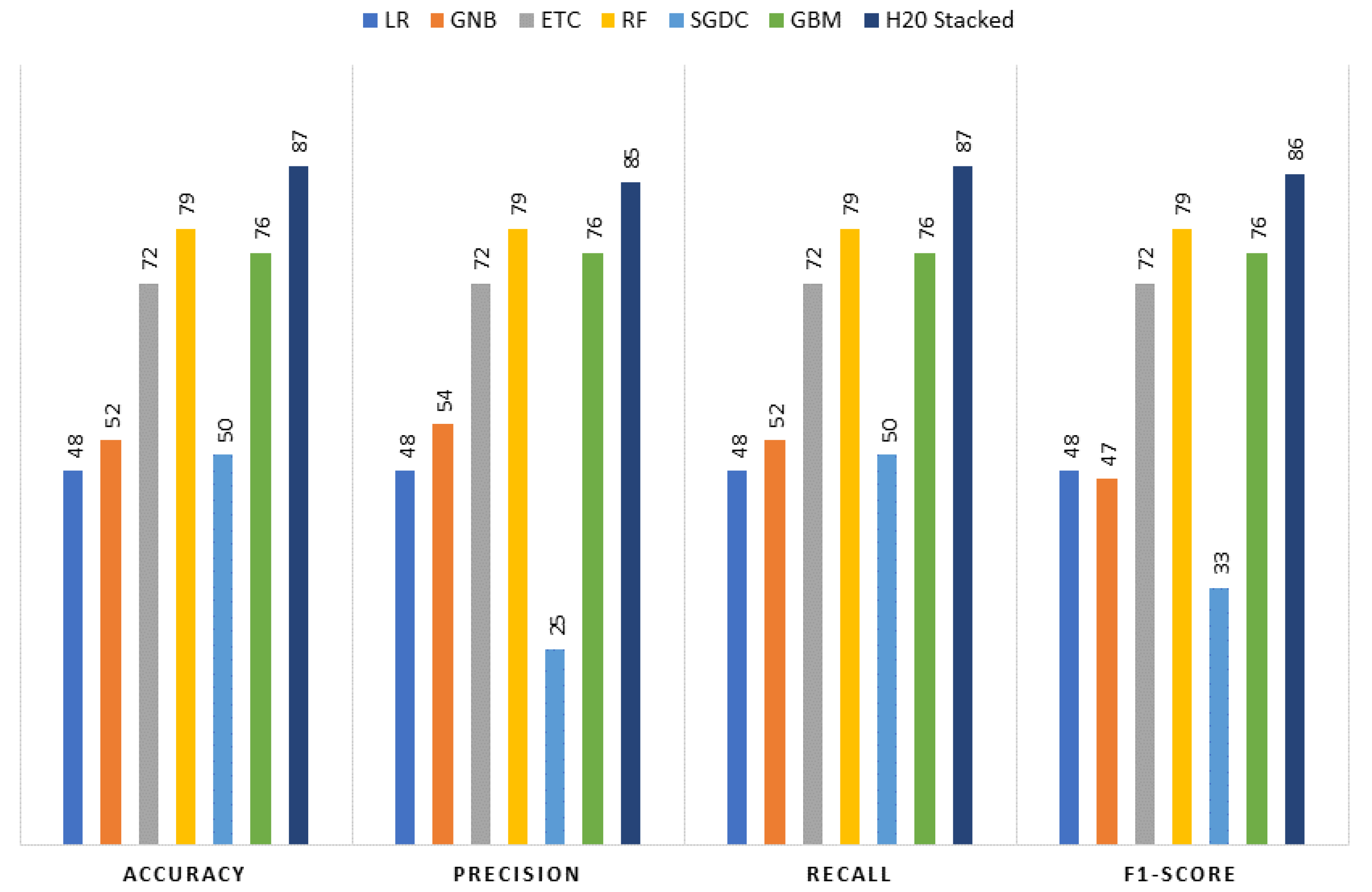
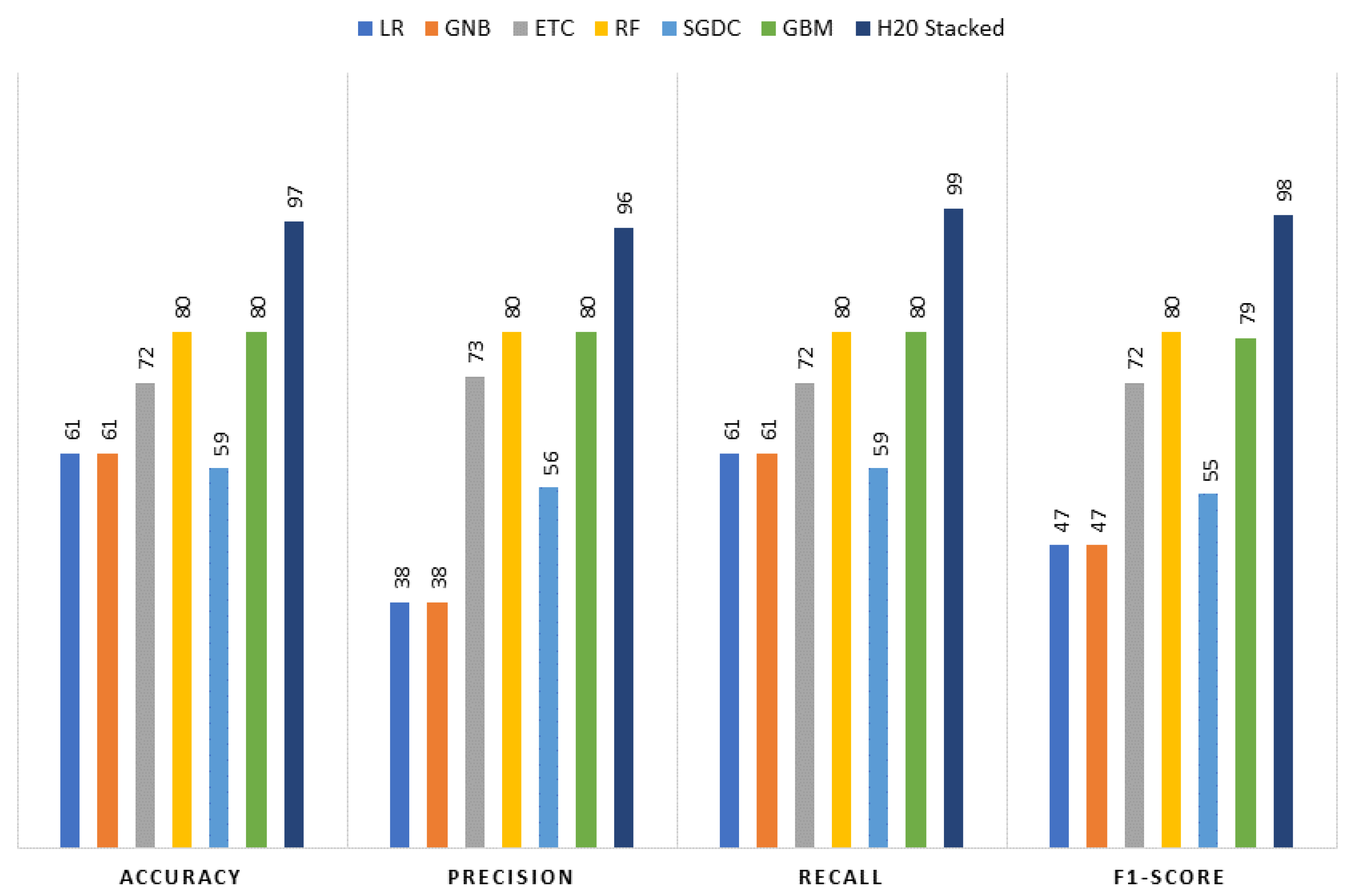
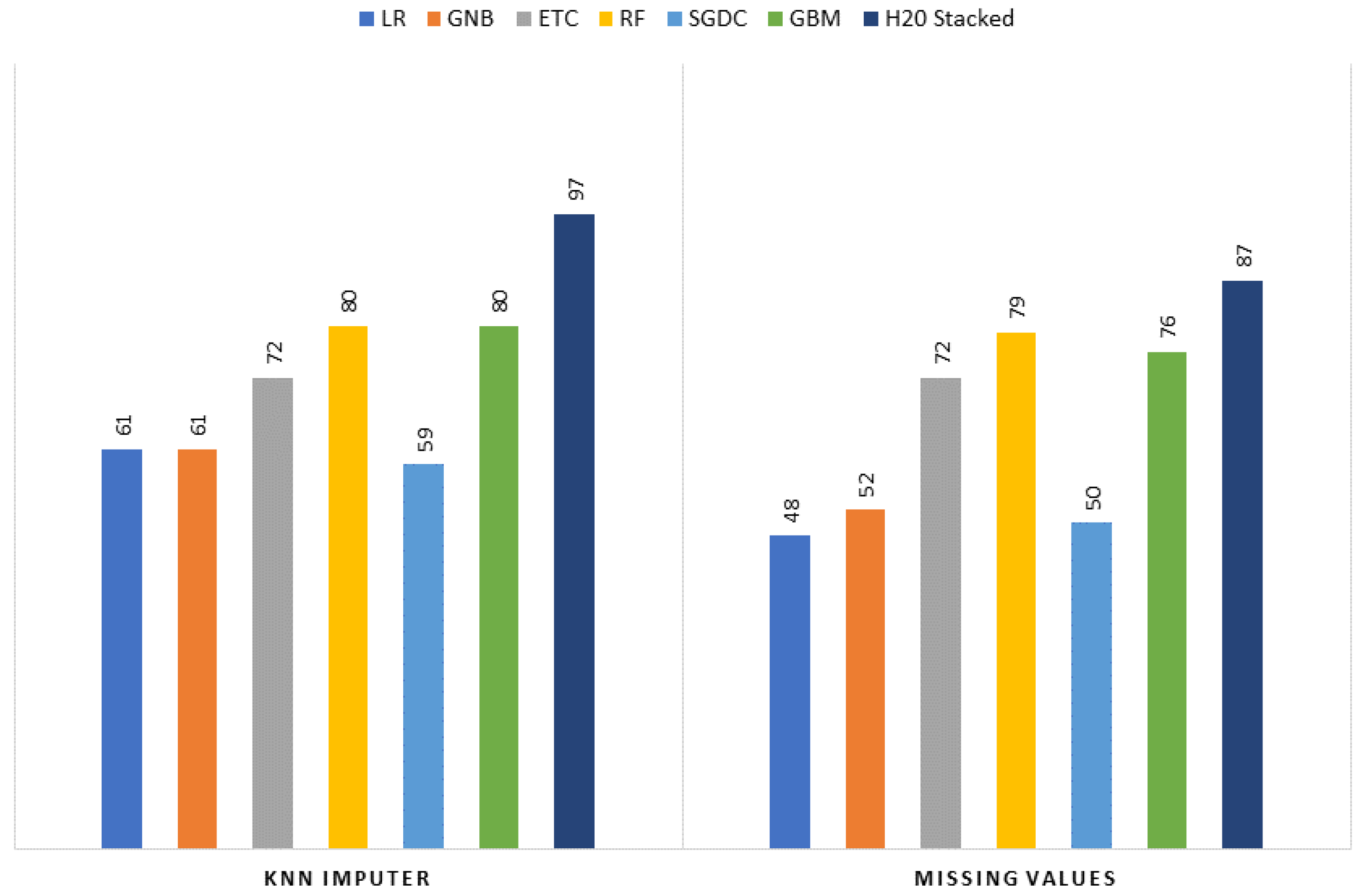
For resolving the issue of missing values, experiments are performed using two scenarios, where the first scenario involves deleting the missing values, while a K nearest neighbor (KNN) imputer is used in the second scenario.
Experiments are conducted to assess the performance of the KNN imputer and the proposed H20 AutoML stacked ensemble model involving the use of several learning models including logistic regression (LR), extra tree classifier (ETC), random forest (RF), stochastic gradient descent classifier (SGDC), Gaussian naïve Bayes (GNB), and gradient-boosting machine (GBM).
The importance of different features is explained using the SHapley Additive exPlanations (SHAP) model.
This study of WQC consists of four further sections:
Section 2 briefly discusses the previous research related to WQC.
Section 3 consists of the description of the dataset, proposed methodology, and description of the machine learning model used in this study.
Section 4 describes the results, and
Section 5 discusses the conclusions of the study.
2. Related Work
Water is one of the most important resources for the existence of life, and human needs are directly linked with the availability of water from both sources (surface and groundwater). Thus, it is very important to have a state-of-the-art system that can classify water quality. Many studies carried out for water-quality classification have provided promising results. The literature review constitutes several previous works that used artificial intelligence systems for water-quality index prediction.
Juna et al. [
10] worked on automatic water-quality prediction using a KNN imputer and MLP. They handled the missing values efficiently and obtained higher performance regarding accuracy. They proposed a nine-layer multilayer perceptron (MLP) system with KNN imputer to deal with the missing values. They also used seven machine learning algorithms for comparison. Experimental results show that the proposed nine-layer MLP achieved an accuracy value of 99% for water-quality prediction using the KNN imputer. A dependable approach was proposed by Nida Nasir et al. [
4] for predicting water quality accurately. The authors used various machine learning and stacked ensemble learning model for water-quality classification via the water-quality index. They used LR, RF, DT, SVM XGBoost, CATBoost, and MLP for this purpose. Results of the study show that CATBoost achieved an accuracy of 94.51%. For water-quality classification, Radhakrishnan and Pillai [
2] used machine learning models. They used three machine learning models, including DT, SVM, and NB, in their study and used multiple datasets. The performance of the machine learning models was compared, and the results revealed that DT achieved better classification accuracy, i.e., 98.50%.
Aldhgani et al. [
11] used a non-linear autoregressive neural network (NARNET) and long short-term memory (LSTM). In addition to these deep learning models, they also used three machine learning models, including NB, SVM, and KNN, for experiments. NARNET and LSTM achieved almost the same accuracy but a slightly different regression coefficient (RLSTM= 94.21%, NARNET = 96.17%), and from machine learning models, SVM achieved an accuracy of 97.01%. Shahra et al. [
12] proposed a deep learning-based system for water-quality classification for water distribution networks. The study aims to achieve high accuracy and keep low time for computation. They used two learning algorithms: ANN and SVM. ANN outperformed the SVM model in terms of accuracy and achieved an accuracy of 94%, whereas SVM achieved an accuracy of 89%.
An adaptive neuro-fuzzy system was proposed by Hadi et al. [
13] for the classification of drinking water into two classes: safe and unsafe. They used a real-time time-series dataset that had four water quality parameters: bacteria count, color, turbidity, and pH. The proposed adaptive neuro-fuzzy system achieved an accuracy of 92% for detecting contaminated data. Abuzir and Abuzir [
14] used j48, MLP, and NB for water-quality classification. They used a dataset that had 10 features. Different feature extraction techniques were used for the dimensionality reduction of the dataset. They experimented with three scenarios: using all features, using five features, and using two features. With all features and with selected features, MLP outperformed the other two learning models.
Hassan et al. [
15] used machine learning and deep learning models for classification of Indian water quality data. The authors used SVM, RF, NN, multinomial logistic regression (MLR), and bagged tree models (BTM). The results revealed that the main features, such as total coliform, biological oxygen demand, dissolved oxygen, conductivity pH, and nitrate, affect the water quality classification. A study by Sillbery et al. [
16] used attribute realization (AR) and SVM for water-quality classification of the Chao Phraya River. When they used AR-SVM on six features of river-water data, they achieved accuracy from 86% to 95%. The study by Ahmed et al. [
17] used four different features, including turbidity, pH, TDS, and temperature, for water-quality prediction. Experimental results show that MLP outperformed the other learning algorithms in terms of accuracy and achieved an accuracy of 85.05% with a (3,7) configuration.
The IoT-based system played a vital role in water-quality classification. Kakkar et al. [
18] used IoT-based devices for the data collection of residential overhead tanks. After data collection, they use machine learning and a deep learning system for WQC. Malek et al. [
19] used Kelantan River data from the years 2005 to 2020 for water-quality classification. They employed different kinds of machine learning models. For water quality, they used 13 physical and chemical parameters. From the experiments, results show that gradient boosting with a learning rate of 0.1 achieved an accuracy value of 94.90%. For water quality and water-demand prediction, Rustam et al. [
20] proposed an artificial neural network system. The authors used an artificial neural network with one hidden layer and several dropouts and activation layers. Experiments were conducted on two datasets to predict water quality and water consumption. For water-quality prediction, they achieved an accuracy of 0.96%, while the
score for water consumption prediction was 0.99%. A comparative analysis of existing approaches for water-quality prediction is presented in
Table 1.
3. Material and Methods
This section explains the proposed approach for predicting water quality, as well as the machine learning models and dataset used in the experiments.
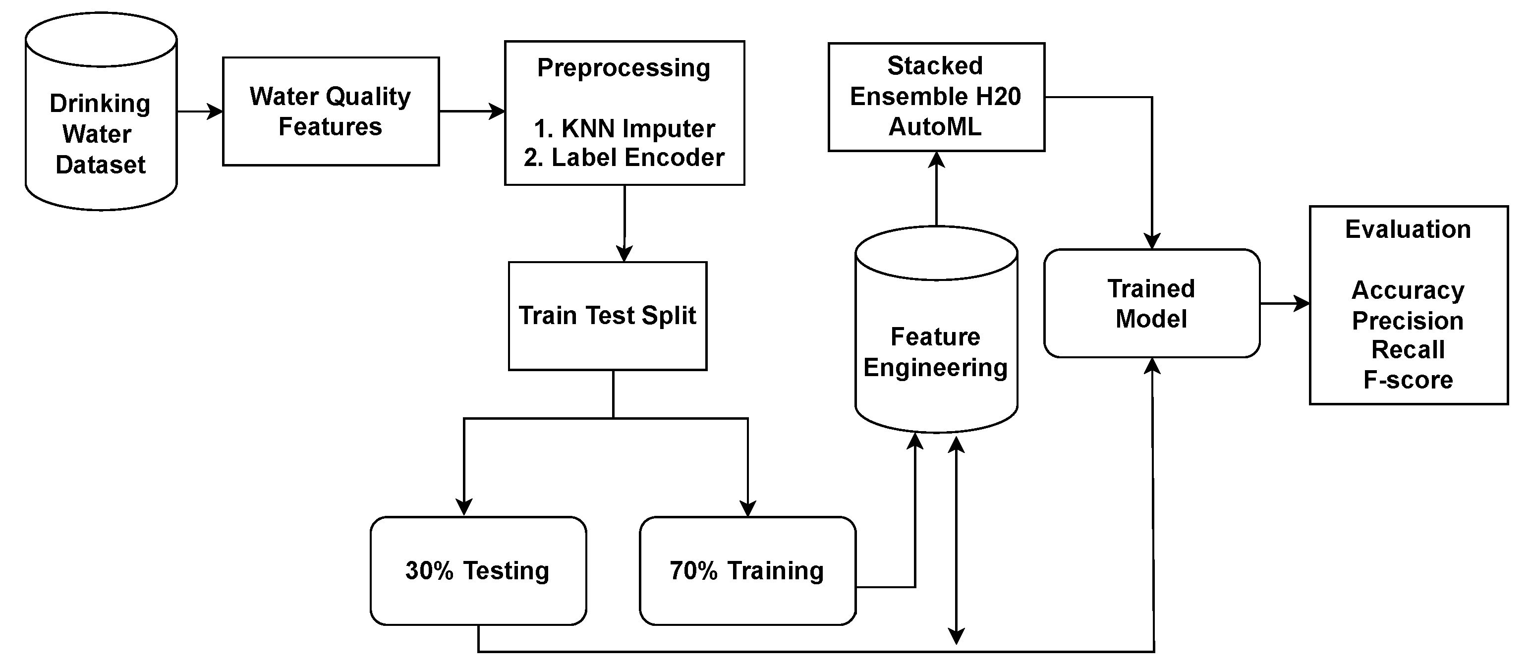
Figure 1 illustrates the proposed architecture used for experiments in water-quality prediction.
3.1. Description of Dataset
The dataset used in this study is obtained from Kaggle, which is a well-known platform. The dataset used in this study is known as “Water Quality”, and it is freely available at [
21]. A brief description of the dataset is given in
Table 2. The dataset constitutes 935 instances and 10 columns with the target class ‘potable’. The target class has two values, 1 and 0, where 1 is used if the water is safe for drinking, and 0 is used if the water is not safe for drinking.
3.2. KNN Imputer
In today’s world, a large amount of data is available to perform research and decision-making. These data are generated from different and heterogeneous sources, so their adequacy and relevancy may vary concerning a research objective. Often, such datasets are limited by missing information for one or more of their attributes. This might happen due to human error with data extraction or collecting or due to erroneous conversions and other processing routines. As a result, dealing with missing values has become an important part of data preparation. The method of imputation is very important, as the performance of the models is directly linked with it. The KNN imputer by sci-kit-learn is a common approach for imputing missing data. It is widely used in place of traditional imputation methods [
22].
KNN imputer facilitates the imputing of missing values in observations by utilizing a Euclidean distance matrix to determine the nearest neighbors. The Euclidean distance is calculated by ignoring missing values and increasing the weight of non-missing coordinates. Euclidean distance can be calculated using the following formula:
where
3.3. Deleting Missing Values from the Dataset
The second approach for dealing with the data is to delete the missing values. This approach is used in the second set of experiments, where all fields with missing data are deleted.
3.4. H2O AutoML
H
O AutoML [
23] is a machine learning algorithm that works automatically and is included in the H
O system [
24]. It is easy to understand and easy to implement, it is for enterprise environments, and it produces high-quality models. On the tabular dataset, H
O AutoML supports multiple kinds of problems, such as binary classification, multi-class classification, and regression problems. The major advantage of H
O AutoML is that it has the capacity for fast scoring; multiple H
O models can produce predictions within very little time. The other benefit of H
O AutoML is that it offers APIs in different languages. Due to these benefits, it is seamlessly used in different fields. For big data analytics, H
O AutoML has a tight integration. H
O AutoML is a fully automatic supervised learning model that is implemented in the H
O library. It is an open-source, distributed, and scalable model; it is widely used in academia and in the industry as well.
To evaluate the performance of the learning models for water-quality detection, several classifiers are used with the H
O AutoML technique to check the efficacy of the proposed system. H
O version 3.10.3.1 is used to train the learning models. All learning algorithms are implemented using the H
O AutoML module. This study uses seven learning models for water quality classification: logistic regression [
25], Gaussian naïve Bayes [
26], random forest [
27], extra tree classifier [
28], gradient boosting machine [
29], stochastic gradient decent [
30], and H
O stacked ensemble [
23].
3.5. Logistic Regression
LR is extensively used for classification. LR has the ability to deal with a large number of features because it provides a straightforward equation for classification problems into a binary class. To achieve the best results, we optimized several of its hyperparameters. To compute the probability of a certain event occurring, a mathematical function called the ’logistic regression hypothesis function’ is used. The sigmoid function is used to transform the logistic regression output value into a probability value. The cost function of LR can be calculated as
3.6. Gaussian Naïve Bayes
GNB is the advanced variant of naïve Bayes; it is also based on the Bayesian theorem. Naïve Bayes handles categorical variables efficiently, so all the variables in naïve Bayes must be categorical. However, the water quality classification dataset consists of numeric data, so that is why we use GNB. GNB uses the partial technique to handle large datasets because during training, GNB takes the chunks of data into account.
3.7. Random Forest
RF is a tree-based ensemble model. It is an advanced version of a decision tree and is used to handle supervised learning problems. RF combines many weak learners, so it produces highly accurate predictions. By using the different bootstrap samples, RF uses the bagging technique for the training of many decision trees by sub-sampling of the training dataset to obtain the bootstrap samples. The size of the bootstrap samples is the same as the size of the training dataset. In RF, the notable issue in the construction of a tree involves attribute identification at each level for the root node; this process is known as attribute selection. In ensemble classification, two or more classifiers are trained, and their results are combined using a voting process. The most-common ensemble techniques are bagging and boosting. RF can be defined as
For the majority of classification tasks, the Gini index is used as a cost function for the estimation of a split in the dataset. The Gini index can be computed using
3.8. Stochastic Gradient Decent
SGD is a renowned optimization method that learns the optimized value of the model’s parameter in each iteration to reduce the cost function (
). SGD is a well-known variant of GD that concerns a random stochastic such that in each iteration it selects a single sample for the training of the model. SGD needs less training time to find the cost function of only a single training sample
at each iteration to attain local minima. It does so by updating the model parameters for every iteration
and target class
.
where
is the model learning rate and
is the parameter. For better performance, SGD uses several hyperparameters.
3.9. Gradient Boosting Machine
GBM is a boosting algorithm that is widely used for classification and regression problems. GBM consists of three main factors: a loss function, a weak learner, and an additive model. The additive model in gradient boosting minimizes the loss function by combining many weak learners. It handles imbalanced datasets efficiently. The purpose of boosting is to enhance the power of the algorithm in such a way that it can detect the model’s weaknesses and replace them with strong learners to produce near-perfect outcomes. GBM does this task by gradually, additively, and sequentially training numerous models.
3.10. Extra Tree Classifier
ETC is an ensemble learning model that is an ensemble of multiple unpruned decision trees. For the splitting nodes, it uses the subset of features. Unlike RF, it uses the whole of the data for construction of the decision tree rather than using the bootstrapping data. There are two primary parameters in ETC: the number of randomized input features selected at each node, the lowest sample size needed for splitting a node , and the ensemble (M) number of decision trees. The decision tree in ETC is very less likely to be correlated because of the randomized selection of points of the split. ETC aggregates the DT predictions in the ensemble to produce the final predictions in the case of regression.
3.11. H2O AutoML Stacked
The stacked ensemble learning model H2O is a supervised learning model that is used to find the optimal combination from a number of prediction algorithms. The process of finding the optimal combination from many prediction algorithms is called stacking. The stacked ensemble model H2O supports any kind of problem, including binary and multi-class classification. It also supports regression problems. This research work leverages an RF classifier as a base and a gradient boosting machine as a meta-estimator to predict the performance of drinking-water quality.
3.12. Explainable Machine Learning
For the advancement of the decision-making sequence, traditional machine learning base prediction needs post hoc interpretations. The function of these post hoc interpretations is so that the community easily understands the rationale that works behind predictions. Machine learning applications emphasize that interoperability is very important, similar to accuracy [
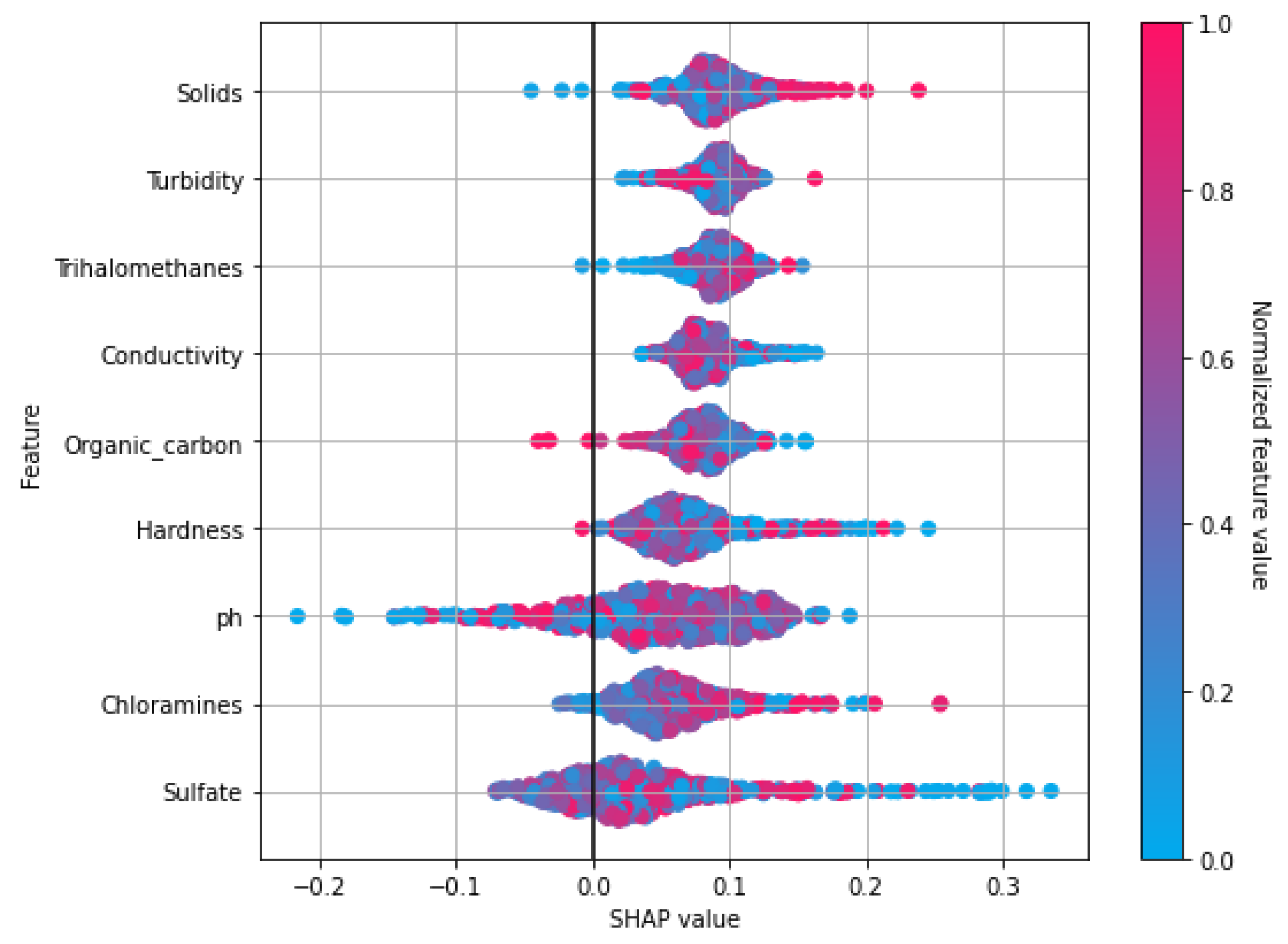
31]. Explainable ML helps in providing the basic add-in to machine learning models by improving the transparency of predictions that are obtained automatically. Foremost, such models are divided into two groups: data-driven interpretation and model-driven interpretation. To interpret machine learning-based predictions, we used the SHAP explainable model because it has the capacity to recognize values as a unified measure of feature importance.
3.13. Shapley Additive Explanations
According to Lundberg and Lee [
32], SHAP is used to explain ML prediction based on game theory. For instance, inputs are taken as players, and predictions are referred to as payout. The contribution of each player in the game can be calculated with the help of SHAP. Several versions of SHAP have been introduced by Lundberg and Lee, including TreeSHAP, KernelSHAP, linearSHAP, and DeepSHAP. These versions are for specific machine learning model categories. For example, in this study, Tree-SHAP is used to explain the ML predictions. Tree-SHAP uses the linear-explanatory model and shapely values for the initial prediction model estimation.
where
represents the basic features,
⌀ denotes the feature attribution, and
shows the explanation model. Lundberg and Lee [
32] calculate each feature attribution using the below equation:
where
represents the set of all inputs,
K shows the input subset of a feature, and
is the expected value of the function on subset
k. A linear additive feature attribute method is used by SHAP for the simpler explanation
3.14. Proposed Framework
This section describes all phases of the proposed approach framework and its modules utilized in the experiment.
Figure 2 elaborates on the proposed framework architecture. The proposed approach has sub-phases, and each phase has been explained separately. The proposed framework consists of two phases. In Phase 1, all the learning algorithms are implemented using H20 AutoML model selection on the dataset containing the missing values. In Phase 2, the dataset is balanced and sparsity is removed using the KNN imputer technique, and then learning algorithms are implemented. The results obtained clearly show the superiority of the H20 stacked ensemble model over the rest. After that, using the SHAP explainable AI technique, the contributions of features toward the prediction are also explained. SHAP reveals the proportion to which each feature participates in the prediction of drinking-water quality. The reason for choosing this stacking is that both these models perform well individually as compared to other models and are suitable for the task at hand. The SHAP technique is used to demonstrate the final prediction with respect to features so as to provide an explanation of the model’s performance.
3.15. Evaluation
The model’s evaluation is the important step that mainly focuses on estimation of the performance of the model on unseen data. For water-quality classification, the four outcomes are described below:
True Positive (TP): instances that are actually positive and are predicted positive.
True Negative (TN): instances that are actually negative and are predicted negative.
False Positive (FP): instances that are negative and are predicted as positive.
False Negative (FN): instances that are positive and are predicted as negative.
This study evaluates the proposed system in terms of accuracy, precision, recall, and F-score. The values of these parameters range between 0 and 1.
Accuracy is the percentage of correctly predicted instances. It can be computed using the following formula:
Precision is the exactness of the classifier. Mathematically, precision can be computed as:
Recall is the completeness of the classifiers. Mathematically, recall can be computed as:
The harmonic mean of recall and precision is called the F1 score. It is also referred to as F-score. It can be calculated using the following formula:
Figure 2.
Proposed stacked ensemble H20 AutoML architecture.
Figure 2.
Proposed stacked ensemble H20 AutoML architecture.


 ,
, 


