The Revised Curve Number Rainfall–Runoff Methodology for an Improved Runoff Prediction

Abstract

The Curve Number (CN) rainfall–runoff model is a widely used method for estimating the amount of rainfall and runoff, but its accuracy in predicting runoff has been questioned globally due to its failure to produce precise predictions. The model was developed by the United States Department of Agriculture (USDA) and Soil Conservation Services (SCS) in 1954, but the data and documentation about its development are incomplete, making it difficult to reassess its validity. The model was originally developed using a 1954 dataset plotted by the USDA on a log–log scale graph, with a proposed linear correlation between its two key variables (I_a and S), given by I_a = 0.2S. However, instead of using the antilog equation in the power form (I_a = S^0.2) for simplification, the I_a = 0.2S correlation was used to formulate the current SCS-CN rainfall–runoff model. To date, researchers have not challenged this potential oversight. This study reevaluated the CN model by testing its reliability and performance using data from Malaysia, China, and Greece. The results of this study showed that the CN runoff model can be formulated and improved by using a power correlation in the form of I_a = S^λ. Nash–Sutcliffe model efficiency (E) indexes ranged from 0.786 to 0.919, while Kling–Gupta Efficiency (KGE) indexes ranged from 0.739 to 0.956. The I_a to S ratios (I_a/S) from this study were in the range of [0.009, 0.171], which is in line with worldwide results that have reported that the ratio is mostly 5% or lower and nowhere near the value of 0.2 (20%) originally suggested by the SCS.

1. Introduction

Floods are natural disasters caused by a large amount of water that overflows a land beyond its normal level. One of the main causes of flooding is the excess rainfall that is not absorbed by the ground or a land surface, which is also known as the runoff amount. When the runoff amount exceeds the capability of the existing flood control infrastructure, overflows of the water will occur, leading to flooding events. Once flooding occurs, it will threaten the lives of the residents, especially those who live in the lower elevated regions. Moreover, the flood will also lead to a huge amount of financial loss, which includes the damage brought by the flood to the victims and financial costs for the government to recover the flood-stricken regions and indemnify the victims of the flood. In addition to impacting human beings, animals will also lose their shelter due to flooding. Thus, a better understanding of the relationship between the rainfall and the runoff amount is crucial to produce a better runoff prediction model. With a better prediction of the runoff amount, government agencies will be able to efficiently plan for the management of flood-related issues. For instance, the government can plan a sufficient amount of flood prevention infrastructure, such as the retention pond, the drainage system, the reservoir, and others, according to the predicted runoff amount with the aim of coping with the possible flood issues.

The change in the runoff depth, or the amount of water that flows over the surface of the land, can be influenced by a number of factors, including climate change, changes in land use, and anthropogenic interventions [1,2,3,4,5]. Some studies have found that both climate change and human activities can contribute to changes in runoff, with climate change having a greater impact in the 1980s and human activities having a greater impact in the 2000s [4]. Other studies have focused specifically on the impact of land use changes, such as urbanization, on runoff depth [3,5]. These studies have found that land use changes, such as converting dryland agriculture to an impervious surface, can increase runoff depth, while converting dryland agriculture or an impervious surface to grass or forest can decrease runoff depth [3]. Additionally, human disturbance such as vegetation restoration projects can also affect the runoff amount [2] while changes in a forest area can also have a significant impact on the change in the runoff regime [1,2,3].

To estimate the rainfall–runoff amount, the United States Department of Agriculture (USDA) and Soil Conservation Services (SCS) developed the Curve Number (CN) rainfall–runoff model in 1954. The CN model was derived based on the maximum rainfall and runoff data that are collected from less than 200 watershed data in 23 different states in the USA. However, the data and documentation about the initial development of the method are not complete, and many datasets have been lost, which poses a great challenge in reassessing the validity of what was used to formulate the SCS’s CN rainfall–runoff model. The SCS developed the method based on data mainly obtained from watersheds monitored with rain and streamflow gauges in the US. [6,7,8,9,10]. With the data and effort from SCS, the SCS’s CN model was developed as follows:

$$\mathrm{Q}=\frac{{\left(\mathrm{P}-{\mathrm{I}}_{\mathrm{a}}\right)}^2}{\mathrm{P}-{\mathrm{I}}_{\mathrm{a}}+\mathrm{S}}$$

(1)

where

Q = Runoff depth (mm).

P = Rainfall depth (mm).

I_a = The initial abstraction amount (mm).

S = Maximum potential water retention of a watershed (mm).

Besides developing the model, the SCS also suggested that I_a = λS, in which λ is the initial abstraction coefficient ratio to relate the I_a and S values. As in 1954, there is a limited amount of rainfall data; thus, this equation was flimsily justified based on daily rainfall and runoff data. The only surviving evidence is documented in a different edition of the Natural Resources Conservation Services’s (NRCS) National Engineering Handbook, Section 4 (NEH-4) [8,9,10].

In addition to the model, the SCS also proposed a fixed constant of 0.2 as the value for the λ, for the equation I_a = λS. Thus, the linear correlation with the form of I_a = 0.2S was introduced to simplify the SCS’s CN model and the calculations. In NRCS NEH-4, there is a note mentioning that the reason for proposing the λ as 0.2 is because 50% of the data points fall between the range of 0.095 < λ < 0.38 [10]. With the substitution of I_a = 0.2S into the SCS’s CN model, Equation (1) will eventually be simplified into the conventional SCS runoff forecast model. The conventional (simplified) SCS rainfall–runoff prediction model is as follows:

$$\mathrm{Q}=\frac{{\left(\mathrm{P}-0.2\mathrm{S}\right)}^2 }{\mathrm{P}+0.8\mathrm{S}}$$

(2)

where the restriction of P > 0.2S must be obeyed, or else there will be no runoff (Q) occurring.

Since the inception of the CN runoff model in 1954, it has gained high acceptance in hydrology studies. The model was also frequently applied to hydrologic problems for which it was not originally designed [11]. The conventional model is commonly introduced in textbooks, certified hydrological manuals, and even incorporated in many software as well as programs since 1954 [12]. The model is also integrated into many USDA SCS systems and hydrology-related models [13]. Since the conventional model is frequently applied to other hydrologic models, the accuracy and the reliability of the model itself can be a major factor that determines the performance of the related software and the reliability of any handbook that is related to the model.

Throughout the years, there are researchers who have questioned the reliability and the accuracy of the hypothesis that proposed the fixed value of 0.2 as the value of λ. Based on the results obtained from different studies based on different regions, different ranges of λ value had been proposed. For example, the US researchers had suggested a range of 0.02 < λ < 0.07 and λ = 0.05 was the best overall value for American watersheds. On the other hand, Australian studies reported that the range of the λ should be around 0.2 or lower [14,15]. This suggested that the λ value will differ accordingly to a different region; thus, the SCS’s hypothesis of fixing the λ value as 0.2 became ambiguous and led to the tendency of the CN runoff model to underpredict or overpredict the runoff amount. Some researchers have overlooked the fact that the λ value is specific to a particular region or watershed and have even directly adopted λ = 0.05 in their studies, even though it was a result from the US [7]. Therefore, it is crucial to develop a model calibration methodology based on the specific rainfall–runoff characteristics of a watershed for SCS practitioners.

In the past six decades, many studies had been carried out to challenge the SCS’s hypothesis, which fixed the λ value at 0.2. There were also studies that tried to determine the optimal λ value for the linear modelling that can improve the accuracy and reliability of the SCS’s CN model.

Reviewing the graphs in Figure 1 (graphs obtained from three different sources), the data points are all plotted on a log–log scale graph. However, the linear correlation with the form of I_a = λS was used to formulate and simplify Equation (1) into (2). This can be a mathematical error or an oversight in the past which leads to the inaccuracy of the model’s runoff predictive ability. Since the SCS’s field data points were plotted on a log–log scale graph, the relation between the two key variables (S and I_a) should be in the power correlation instead of a linear correlation.

To date, SCS curve number rainfall–runoff-related studies either evolved around its basic model (Equation (1)) calibration or added new variable(s) to create a runoff model variant. No published work has explored other possible correlations between I_a and S and assessed the impact to its rainfall–runoff mechanism yet. Equation (2) exists in all hydrology textbooks; it also led to curve number derivation and has been applied in many designs while many types of software incorporated I_a = 0.2S in their algorithms. If I_a and S correlate otherwise, it will change the whole model and the way SCS curve number theory is taught. If the fundamental core theory of the SCS curve number rainfall–runoff model changed, the model and all its related downstream information will have to be re-derived.

2. Materials and Methods

2.1. Validity of the Linear Correlation (I_a = 0.2S) and Introduction of I_a = S^λ

A previous study reassessed the use of the linear correlation of “I_a = 0.2S” based on the 1954 SCS original dataset and rejected the validity of the linear correlation model of the form I_a = 0.2S, at alpha level = 0.01. Instead of a constant of λ = 0.2, the study proved that the best linear model for the 1954 SCS original dataset should be I_a = 0.112S [16], which is also in line with the best regressed linear equation of I_a = 0.111S reported in another study [17]. As the linear correlation of I_a = 0.2S was reported as not statistically significant when reevaluated using the original 1954 SCS field data, the SCS rainfall–runoff predictive model Equation (1) should be recalibrated before it is used.

As supported by the power law, if the independent variables and dependent variables were linearly correlated to each other on a log–log scale graph, then a power regression equation will be able to correlate both the variables, in terms of the normal scale. Since the best-fitted linear equation for the 1954 SCS original dataset was reported as I_a = 0.112S or I_a = 0.111S in the past two studies [16,17], the best fitting model for the same datasets in a normal scale should be in the power model with the form of I_a = S^0.112 or I_a = S^0.111 to simplify Equation (1).

Since Equation (2) had been proven to be insignificant at the alpha level of 0.01 by past studies [16,17], rederiving the model will be compulsory to ensure the precision of the model’s runoff predictions. There is no new evidence to suggest a different correlation between I_a and S due to the SCS’s incomplete documentation and missing datasets. Thus, this study adopted the model calibration technique developed in our past studies and thoroughly assessed the use of the power correlation equation in the general form of I_a = S^λ to simplify the SCS’s CN base model, Equation (1), and recalibrate the runoff prediction model based on the regional rainfall–runoff dataset using inferential statistics.

2.2. Study Site and Models’ Performance

In this study, the reliability and performance of the recalibrated rainfall–runoff model were tested using datasets from different locations in Malaysia and datasets from two previous studies in China and Greece. In Malaysia, the Department of Irrigation and Drainage’s Hydrological Procedure no. 11 (DID-HP 11) collected 474 rainfall–runoff data pairs from 1964 to 2016 from watersheds throughout Malaysia, while the Hydrological Procedure no. 27 (DID-HP 27) collected 227 rainfall–runoff data pairs from 1970 to 2000 [18,19]. The study also combined the DID-HP 11 and 27 datasets (consisting of 701 data pairs collected from 1970 to 2016) in the analysis. In addition, 72 rainfall–runoff data pairs collected at the Kerayong watershed in Kuala Lumpur, Malaysia, and 93 data pairs from the Kayu Ara watershed in the Petaling Jaya area of Malaysia were included to test the performance of the recalibrated model [20,21]. Data from two journals were also used in this study: 29 rainfall–runoff data pairs (1994 to 1996) from the Wang Jia Qiao watershed in the Zigui County of Hubei Province, China, [7] and 76 rainfall–runoff data pairs from Attica, Greece [22]. Figure 2 shows the locations from which the rainfall–runoff data were collected.

For purposes of the study, the statistically significant total abstraction value (S), the initial abstraction ratio coefficient (λ), and the corresponding 99% Confidence Interval (CI) for both S and λ will be derived via the Bootstrapping method—BCa procedure (with 2000 samples) at alpha = 0.01, by using the IBM Predictive Analytics software (PASW) version 18.0 (commonly known as SPSS)—as the values will be later used for the calculation of the Curve Number (CN) value.

The main reason for applying the bootstrap BCa technique is because of its robustness and data-distribution-free nature, which is suitable for rainfall–runoff data analysis. Additionally, the bootstrap BCa analytical module is available in SPSS, which is conveniently used to carry out the necessary analysis for this study. The BCa technique also has the ability to correct biases when identifying the confidence interval of the variable of interest at a specific alpha level for further statistical assessments [21,23,24,25,26]. Two normality tests (Kolmogorov–Smirnov and Shapiro–Wilk) are also available in SPSS with the bootstrap BCa confidence interval to identify whether the mean or median CI should be chosen to identify the optimal S and optimal λ for each dataset. If the dataset is not normally distributed, the median CI will be chosen for variable optimization and vice versa.

To make sure the overall prediction results were not biased against any of the datasets, the calibration of the SCS runoff model in identifying the optimum value of λ and S based on each P–Q data pair was set to fulfil the model prediction bias at zero level. With the zero bias optimization constraint, the supervised numerical algorithm is proceeded to identify the optimum λ value and optimum S value, within the bootstrap BCa 99% confidence interval. The performance and the predictive accuracy of the models were later assessed for each dataset based on the Nash Sutcliffe Index (E). The Nash Sutcliffe Index is a hydrology model efficiency indicator, in which E = 1 means the model is an ideal model for the prediction, while E < 0 shows the model performance is unacceptable [27,28,29]. The model bias value of 0 indicates that the model is an ideal, error-free model. Both the Nash Sutcliffe Index and Bias can be calculated via Equations (3) and (4) as shown below:

$$\mathrm{E}=1-\frac{{{\displaystyle \sum }}_{\mathrm{i}=1}^{\mathrm{n}}{\left({\mathrm{Q}}_{\mathrm{predicted}}-{\mathrm{Q}}_{\mathrm{observed}}\right)}^2}{{{\displaystyle \sum }}_{\mathrm{i}=1}^{\mathrm{n}}{\left({\mathrm{Q}}_{\mathrm{predicted}}-{\mathrm{Q}}_{\mathrm{mean}}\right)}^2}$$

(3)

$$\mathrm{BIAS}=\frac{{{\displaystyle \sum }}_{\mathrm{i}=1}^{\mathrm{n}}{\left({\mathrm{Q}}_{\mathrm{predicted}}-{\mathrm{Q}}_{\mathrm{observed}}\right)}^{ }}{\mathrm{n}}$$

(4)

There is another metric, known as the Kling–Gupta Efficiency (KGE), that has been proposed to evaluate the performance of rainfall–runoff models. This metric is derived from the Nash Sutcliffe Index and comprises three components: correlation, variability bias, and mean bias [30]. The KGE is frequently used by hydrologists to calibrate and assess the accuracy of rainfall–runoff models [30]. It can be calculated using the following equation:

$$\mathrm{KGE}=1-\sqrt{{\left(r-1\right)}^2+{\left(\frac{{\sigma }_{sim}}{{\sigma }_{obs}}-1\right)}^2+{\left(\frac{{\mu }_{sim}}{{\mu }_{obs}}-1\right)}^2}$$

(5)

where

r = linear correlation between observations and simulations

${\sigma }_{sim}$ = standard deviation of the simulations

${\sigma }_{obs}$ = standard deviation of the observations

${\mu }_{sim}$ = mean of simulations

${\mu }_{obs}$ = mean of observations

Similar to the E Index, a value of 1 for the KGE indicates a perfect match between observed and simulated data [30]. A KGE value greater than -0.41 suggests that the model is performing better than the mean flow benchmark [30].

Unlike in our past studies, the general formula for S was rearranged from Equation (1) with I_a = λS to determine the value of S using the values of P and Q data pairs with a closed-form expression for S [7,14,15,21,29]. However, with the introduction of the power model I_a = S^λ, the general formula for S does not have a closed-form expression in this study, so a numerical analysis technique will be applied to obtain the value of S. (The derivation and simplification of the general formula for S based on the power regressed model are summarized in Appendix A.) As a result, the simplified S general formula obtained was as follows:

$${(2{\mathrm{S}}^{\lambda }+\mathrm{Q}-2\mathrm{P})}^2=4\mathrm{SQ}+{\mathrm{Q}}^2$$

(6)

The numerical analysis technique will need to be carried out on Equation (6) to identify the optimal λ and S value, denoted by S_λ, according to the P and Q data pairs of the respective study sites. Besides the S_λ values obtained from Equation (6) via the numerical analysis technique, the S_0.2 values for each of the P–Q data pairs for all the study sites were also determined based on the S general equation that was introduced in the previous study, where the linear correlation was applied, with the form of I_a = 0.2S to simplify and formulate the current SCS runoff predictive model [6,7,14,15,16,17,21,29]. (The S general Equation that was used to obtain the S_0.2 values was summarized in Appendix B.) The S general equation that was used to obtain the S_0.2 values was shown as follows:

$${\mathrm{S}}_{0.2}=5\left(\mathrm{P}+2\mathrm{Q}-\sqrt{4{\mathrm{Q}}^2+5\mathrm{PQ} }\right)$$

(7)

Once the S_λ and S_0.2 values were obtained with Equations (6) and (7) according to the corresponding P and Q data pairs, the best correlation between S_λ and S_0.2 and the corresponding best correlation equation can be mapped via the SPSS model regression module for a study site. When the optimal λ value is different from the conventional value of λ = 0.2, a correlation between the newly found λ value and 0.2 must be used to calculate the curve number again [7,11,14,16,21,29]. Therefore, it is important to identify the best correlation between S_λ and S_0.2 and then convert the S_λ back to the equivalent S_0.2 value to derive the conventional SCS curve number (CN_0.2) value that SCS practitioners are familiar with for routine application. The best correlation between S_λ and S_0.2 is determined by the highest adjusted R square value (R²_adj), the lowest standard error of the estimate, and a model with a significant p value, which can be determined in SPSS through the regression module [31,32]. (The approach is summarized in Appendix C.)

For example, the best correlation equation from SPSS between S_λ and S_0.2 for the Kerayong watershed, Malaysia, was identified in SPSS as follows:

S_0.2 = 3.223 S_0.199^0.355

(8)

As introduced by the SCS, the equation to calculate the SCS curve number value is shown below:

$${\mathrm{CN}}_{0.2}=\frac{25,400}{254+{\mathrm{S}}_{0.2}}$$

(9)

CN_0.2 = Conventional Curve Number, Curve number of λ = 0.2.

S_0.2 = Total abstraction amount of λ = 0.2 (mm).

At the same time, Equation (9) can be rearranged into Equation (10):

$${\mathrm{S}}_{0.2}=254\left(\frac{100}{{\mathrm{CN}}_{0.2}}-1\right)$$

(10)

By substituting the best correlation equation (Equation (8)) back to the SCS curve number (Equation (9)), the conventional curve number for the study site can be calculated accordingly:

$${\mathrm{CN}}_{0.2, \mathrm{Kerayong}}=\frac{25,400}{254+\left[3.223 {\left({\mathrm{S}}_{0.199}\right)}^{0.355}\right]}$$

(11)

The correlation equation that correlates both S_λ and S_0.2 will be very crucial as it will directly affect the overall performance of the rainfall–runoff model derived from the power regressed model. The correlation equation is also the key to convert S_λ back to its equivalent S_0.2 value for the calculation of CN_0.2 for SCS practitioners [29,32].

3. Results

3.1. Study Site and Models’ Performance

In this study, the S and λ values were calculated for every dataset based on each corresponding P and Q value. Then, both the Kolmogorov–Smirnov and Shapiro–Wilk tests were carried out to test the normality of each dataset. Both λ and S were not normally distributed (ρ < 0.001) for all the datasets except for Wang Jia Qiao watershed in China. The Kolmogorov–Smirnov and Shapiro–Wilk tests on the λ values showed a significance level of 0.319 and 0.2, which means that the λ values were normally distributed while S values were not normally distributed for Wang Jia Qiao’s dataset (ρ < 0.01). This normality analysis in this study later helps in determining the optimal S value and λ value for each dataset based on the power regression correlation (I_a = S^λ) within the 99% Confidence Interval of both S and λ values, accordingly [7,21,29,33,34]. Once the optimal S value and λ value were obtained for each corresponding dataset, the runoff prediction model can be formulated (refer to Appendix C section for model formulation guide) and the performance for each model can be analyzed.

Table 1. Inferential Statistics of all the datasets, including DID-HP 27, DID-HP 11, the combination of DID-HP 27 and DID-HP 11, Kerayong, Kayu Ara, Attica, and Wang Jia Qiao.

Dataset & Location	E	N	Bias (mm)	KGE	Sλ (mm)	Ia = Sλ (mm)	Ia/S
DID HP 11, Malaysia	0.823	474	2.35	0.805	139.48	3.71	0.027
DID HP 27, Malaysia	0.919	227	0.65	0.956	165.94	2.33	0.014
DID HP 11+27, Malaysia	0.875	701	2.535	0.863	143.99	3.19	0.022
Kayu Ara, Malaysia	0.810	94	0	0.865	24.79	2.20	0.089
Kerayong, Malaysia	0.888	73	0	0.818	9.08	1.55	0.171
Attica, Greece	0.786	77	0	0.798	23.73	1.85	0.078
Wang Jia Qiao, China	0.795	29	0	0.739	386.57	3.57	0.009

shows the inferential statistics, which include the Nash Sutcliffe index (E), optimal S (S), optimal λ, initial absorption (I_a), and the ratio of I_a to S, for each corresponding dataset.

All models were optimized under a bias value = 0 constraint, except for DID HP 11, DID HP 27, and DID HP 11+27, as those models were unable to obtain bias = 0 within their 99% BCa CI. Therefore, those models were optimized to obtain the maximum E Index. The E and KGE indexes showed good results for all datasets, with the E index ranging from 0.786 to 0.919 and the KGE index ranging from 0.739 to 0.956. The initial absorption (I_a) for each corresponding dataset was determined using the newly proposed power correlation of I_a = S^λ. The ratios of I_a to S values were calculated to benchmark against past study results. The I_a to S ratios (I_a/S) for each study site were in the range of [0.009, 0.171], which is in line with past results that reported that the ratio of I_a to S was mostly 5% or lower and nowhere near the value of 0.2 (20%) as initially suggested by the SCS to simplify the SCS runoff predictive framework into Equation (2) [6,7,11,12,13,14,15,16,17,21,22,29,32,33,34].

The best-fitted correlation equation that correlates S_λ to S_0.2 for each dataset was modelled via SPSS. To measure the fitness of the correlation equation to the datasets, the adjusted coefficient of determination (R²_adj) for each corresponding equation was also identified, together with the ρ-value. The SCS practitioner(s) was taught to choose the CN value from the NEH handbook according to the land use or land cover condition of the watershed and to calculate the S value from Equation (9) or (10) directly; however, it is no longer applicable as the linear correlation of I_a = 0.2S was proven invalid [7,16,17,21,29,33,34]. Thus, the best-fitted correlation equation between S_λ and S_0.2 proposed herewith should be used by the SCS practitioners, in which the optimal S value of each dataset must be converted back to the equivalent S_0.2 value via the mapped correlation equation (

Table 2. Adjusted coefficient of determination (R²_adj) and ρ-value of all the datasets’ correlation equations, including DID-HP 27, DID-HP 11, the combination of DID-HP 27 and DID-HP 11, Kerayong, Kayu Ara in Malaysia, Attica in Greece, and Wang Jia Qiao in China. Power correlation models were identified as the best correlation model in SPSS with the lowest standard error of estimate.

Dataset & Location	Correlation Equation	R2adj	p-Value
DID HP 11, Malaysia	S0.2 = S0.2650.878	0.977	<0.001
DID HP 27, Malaysia	S0.2 = S0.1660.874	0.997	<0.001
DID HP 11+27, Malaysia	S0.2 = S0.2340.880	0.998	<0.001
Kayu Ara, Malaysia	S0.2 = 4.263 S0.2460.438	0.893	<0.001
Kerayong, Malaysia	S0.2 = 3.223 S0.1990.355	0.849	<0.001
Attica, Greece	S0.2 = 5.057 S0.1940.357	0.846	<0.001
Wang Jia Qiao, China	S0.2 = S0.2140.702	0.975	<0.001

) prior to calculate the CN_0.2 value of a watershed [7,21,29,32,33,34] from Equation (9) or (10), as shown in the aforementioned example to derive Equations (8) and (11). SCS practitioners no longer have to decide and choose the CN value from any handbook; they can derive the CN value of a specific watershed according to the regional rainfall–runoff conditions.

3.2. Derivation of Curve Number and Its Confidence Interval

The Bootstrapping BCa 99% CI for the S value of each dataset and the correlation between S_λ and S_0.2 were determined using SPSS in this study. The BCa 99% CI for the corresponding CN_0.2 value of each dataset can then be calculated once the respective correlation equation between S_λ and S_0.2 from Table 2 is substituted into Equation (9) or (10) to derive the equivalent CN_0.2 range (refer to derivation steps in Appendix C), as shown in

Table 3. Bootstrapping BCa 99% CI for the S value and CN_0.2 value of all the datasets’ correlation equations, including DID-HP 27, DID-HP 11, the combination of DID-HP 27 and DID-HP 11, Kayu Ara, Kerayong, Attica, and Wang Jia Qiao.

Datasets	BCa 99% Confidence Interval
S & Curve Numbers	S0.2 (mm)		CN0.2
Dataset & Location	Lower	Upper	Lower	Upper
DID HP 11, Malaysia	100.99	139.48	76.88	81.54
DID HP 27, Malaysia	118.65	165.94	74.46	79.62
DID HP 11+27, Malaysia	115.01	143.98	76.21	79.60
Kayu Ara, Malaysia	20.75	331.07	82.43	94.04
Kerayong, Malaysia	8.77	397.55	90.40	97.33
Attica, Greece	23.73	314.15	86.57	94.19
Wang Jia Qiao, China	289.86	553.69	75.08	82.60

. Table 2 lists the best regressed correlation equation identified in SPSS while Table 3 summarizes the Bootstrapping BCa 99% CI for the S value and the calculated CN_0.2 value range of each dataset in this study.

4. Discussion

4.1. Validity of the Linear Correlation (I_a = 0.2S) and Introduction of Power Regression (I_a = S^λ)

The Soil Conservation Services Curve Number (SCS CN) method is a widely used method for predicting runoff from precipitation in hydrology studies. It is based on the assumption of a linear relationship between infiltration and soil moisture storage, which is used to estimate the amount of runoff that will occur during a storm event. However, the accuracy and consistency of the SCS CN method have been questioned by many researchers due to concerns about the underlying assumptions and the limited range of conditions under which it has been tested.

Two past studies assessed the linear correlation proposed by the SCS and concluded that I_a = 0.2S was statistically invalid even to its own dataset [16,17]. In 1954, the SCS introduced the linear correlation (I_a = 0.2S) to simplify the SCS rainfall–runoff model into the conventional SCS runoff prediction Equation (2) that is in use until today. However, worldwide studies reported runoff prediction accuracy and consistency issues with the model [6,7,11,12,13,14,15,16,17,21,22,29,30,31,32,33,34]. This simplification may have introduced an inherent risk of Type 2 error into the SCS CN model. (A Type 2 error, also known as a false negative, occurs when a statistical test fails to reject the null hypothesis when it is actually false.) In the context of the SCS CN model, this means that the model may incorrectly predict the runoff amount. The risk of Type 2 error in the SCS CN model has potential implications for downstream derivations and extended applications of the model in hydrology. Researchers and practitioners who use the SCS CN model should be aware of this risk and carefully evaluate the assumptions and limitations of the model in order to ensure the accuracy and reliability of their results.

The 1954 SCS original dataset was plotted on a log–log scale graph, but the SCS adopted a linear correlation to correlate both S and I_a directly to simplify its model framework without taking the antilog form [8,9,10]. In the authors’ opinion, it is possible that the antilog correlation form was not used in the past due to technical limitations in simplifying Equation (1) with I_a = S^0.2 without the use of computers, or the fundamental mathematical mistake was overlooked. Two past studies reassessed the correlation between S and I_a according to the 1954 SCS original dataset and reported that the best correlation equation should be I_a = 0.111S or I_a = 0.112S on the log–log scale graph [16,17]. As such, the antilog form or the power regression equations of I_a = S^0.111 or I_a = S^0.112 will be better correlation equations to the SCS original dataset as compared to what the SCS had proposed (I_a = 0.2S). This finding necessitated the development of a revised form of the SCS rainfall–runoff model that incorporates the power correlation between I_a and S in the general form of I_a = S^λ to simplify Equation 1 and rederive a new SCS runoff predictive model. The calibration of the SCS rainfall–runoff model (Equation (1)) can be performed based on the newly proposed power regressed model according to the regional or watershed specific rainfall–runoff dataset to improve the runoff prediction accuracy.

The SCS CN basic model is in the form of Q = f(P, λ, S), so there are only two key parameters for optimization. In contrast to previous studies that calibrated the SCS CN model with the I_a = λS equation according to watershed-specific rainfall–runoff datasets using inferential statistics and reported that λ = 0.2 was not statistically significant at the alpha = 0.05 level for modeling runoff [7,16,21,29,33,34], the novelty of this study is to calibrate the SCS CN model with I_a = S^λ and formulate new CN runoff prediction models. To date, no other researchers have attempted to do this.

This study preserved its fundamental framework without adding any new parameters in order to study the possibility of using I_a = S^λ to calibrate and formulate the runoff predictive model. It is noteworthy to highlight that although Equation (2) was able to achieve attractive E and KGE index values (Appendix D,

Table A2. Conventional SCS CN models’ runoff prediction comparison for each study site.

Datasets	SCS Model (Equation (2))			Remark
	E	BIAS	KGE
DID HP 11, Malaysia	0.839	−6.104	0.759	Ia > 60 rainfall data (12.7%)
DID HP 27, Malaysia	0.910	−4.085	0.895	Ia > 6 rainfall data (2.6%)
DID HP 11+27, Malaysia	0.879	−4.451	0.863	Ia > 68 rainfall data (9.7%)
Kayu Ara, Malaysia	0.805	−1.162	0.831	Ia > 6 rainfall data (6.5%)
Kerayong, Malaysia	0.891	−0.885	0.843	Ia > 2 rainfall data (2.8%)
Attica, Greece	0.780	−1.846	0.784	Ia > 5 rainfall data (6.6%)
Wang Jia Qiao, China	0.482	1.586	0.418	Ia > 4 rainfall data (13.8%)

Note: 𝛌 = 0.2 is not significant at α = 0.05 level for any dataset. SCS CN theory requires I_a < rainfall depth (P).

) in certain datasets, the λ value of 0.2 was not significant even at α = 0.05 level for any dataset in this study. As such, the conventional SCS simplified model (Equation (2)) is not statistically significant for modelling any rainfall–runoff in this study. All SCS models have a tendency to underpredict runoff in this study. Additionally, the I_a value of all SCS models violated a requirement from the SCS CN theory which states that there will be no runoff when the rainfall depth (P) is less than the I_a value. Table A2 tabulates the total count of rainfall–runoff data pairs where the recorded P value is less than the SCS model’s I_a value. In contrast, none of the newly formulated power models have this issue.

4.2. Application of the Power Regression Model at Different Study Sites

In this study, datasets were collected from Malaysian watersheds (DID-HP 11 and DID-HP 27, Kerayong and Kayu Ara watershed in Kuala Lumpur area) while two past study datasets were adopted from the Attica watershed in Greece and the Wang Jia Qiao watershed in China. The analytical results showed that the power regression model is able to obtain high runoff predictive ability at all study sites consistently (Appendix D,

Table A1. Power models’ runoff prediction comparison for each study site.

Datasets	New SCS (Power) Model			Remark
	E	BIAS	KGE
DID HP 11, Malaysia	0.823	2.347	0.805	Ia < min rainfall data
DID HP 27, Malaysia	0.919	0.647	0.956	Ia < min rainfall data
DID HP 11+27, Malaysia	0.875	2.531	0.863	Ia < min rainfall data
Kayu Ara, Malaysia	0.810	0	0.865	Ia < min rainfall data
Kerayong, Malaysia	0.888	0	0.818	Ia < min rainfall data
Attica, Greece	0.786	0	0.798	Ia < min rainfall data
Wang Jia Qiao, China	0.795	0	0.739	Ia < min rainfall data

) when compared to the conventional SCS runoff predictive model (Equation (2)). The calculated ratio values of I_a to S (I_a/S) for all the study sites were in the range of [0.009, 0.171] (Table 1) which is in line with past results whereby the ratios were mostly 5% or lower and nowhere near to the value of 0.2 (20%) as initially suggested by the SCS [6,7,11,12,13,14,15,16,17,21,22,29,32,33,34]. It is in line with the results of the largest scale of field tests on the SCS CN model, which analyzed more than half a million rainfall events across 24 states in the USA and reported that I_a/S values were mostly below 5% to achieve better runoff modeling results in American watersheds [17,29,32]. Using the revised CN model may allow for more accurate and reliable predictions of runoff in different types of soils and hydrological conditions. This can be particularly useful for water resource management, as it allows for more informed decision making about the availability of water for various uses and the potential for flood hazards. It is important for researchers and practitioners to be aware of the revised form of the SCS rainfall–runoff model and to consider its use in their work.

4.3. Application of Machin-Learning Techniques to the Rainfall Runoff Model

In recent decades, there has been a significant increase in the use of machine learning in hydrology studies in Latin America and the Caribbean (LAC) [35,36,37,38]. Researchers have introduced various machine-learning techniques, such as long short-term memory (LSTM), Adaptive Neuro-Fuzzy Inference System (ANFIS), Multilayer Perceptron (MLP), Wavelet Neural Network (WNN), Ensemble Prediction Systems (EPS), Support Vector Machine (SVM) and Support Vector Regression (SVR), and Artificial Neural Networks (ANN), to improve the accuracy and performance of predictive models [35]. Hybrid machine-learning approaches, such as ANFIS and WNN, have also been found to have improved accuracy and performance for long-term and short-term rainfall–runoff models [35]. Machine learning can also be used to overcome the issue of lacking time series data for flow hydrographs due to the absence of gauged stations by utilizing flood modelling methods such as the reverse flood routing model, HEC-RAS, and GIS flood maps [38]. It is possible that machine-learning techniques can be combined with the newly proposed rainfall–runoff model from this study.

5. Conclusions

This study proposed a new correlation model to improve the accuracy of the SCS (Soil Conservation Service) rainfall–runoff predictive model, using inferential statistics. The key findings of the study are as follows:

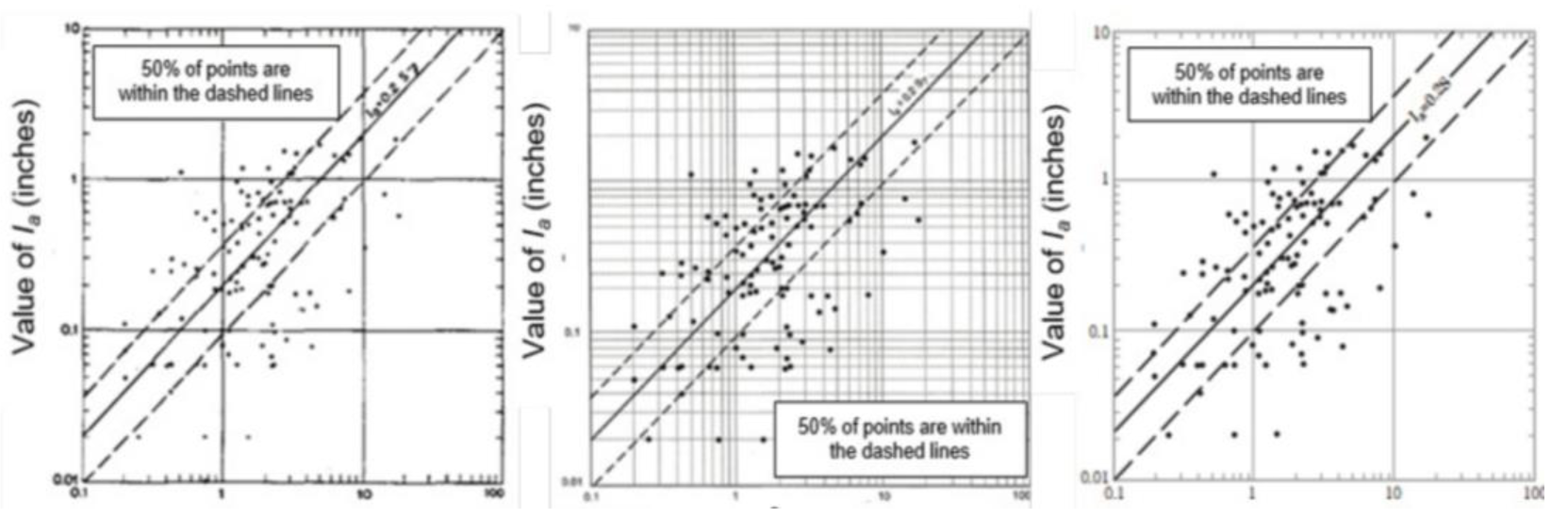
• The linear correlation hypothesis (I_a = 0.2S) proposed by the SCS was found to be statistically invalid, even in the 1954 original dataset. Therefore, it is important to revise the current conventional SCS runoff prediction model to better prepare for the challenges posed by climate change conditions. The use of I_a = 0.2S to simplify equation (1) into the conventional SCS runoff model (equation 2) may have been an oversight in 1954. The power correlation equation (I_a = S^0.111 or I_a = S^0.112) should be used to simplify the 1954 SCS runoff model equation (1) and derive the runoff predictive model, as the original SCS dataset was plotted on a log–log graph.
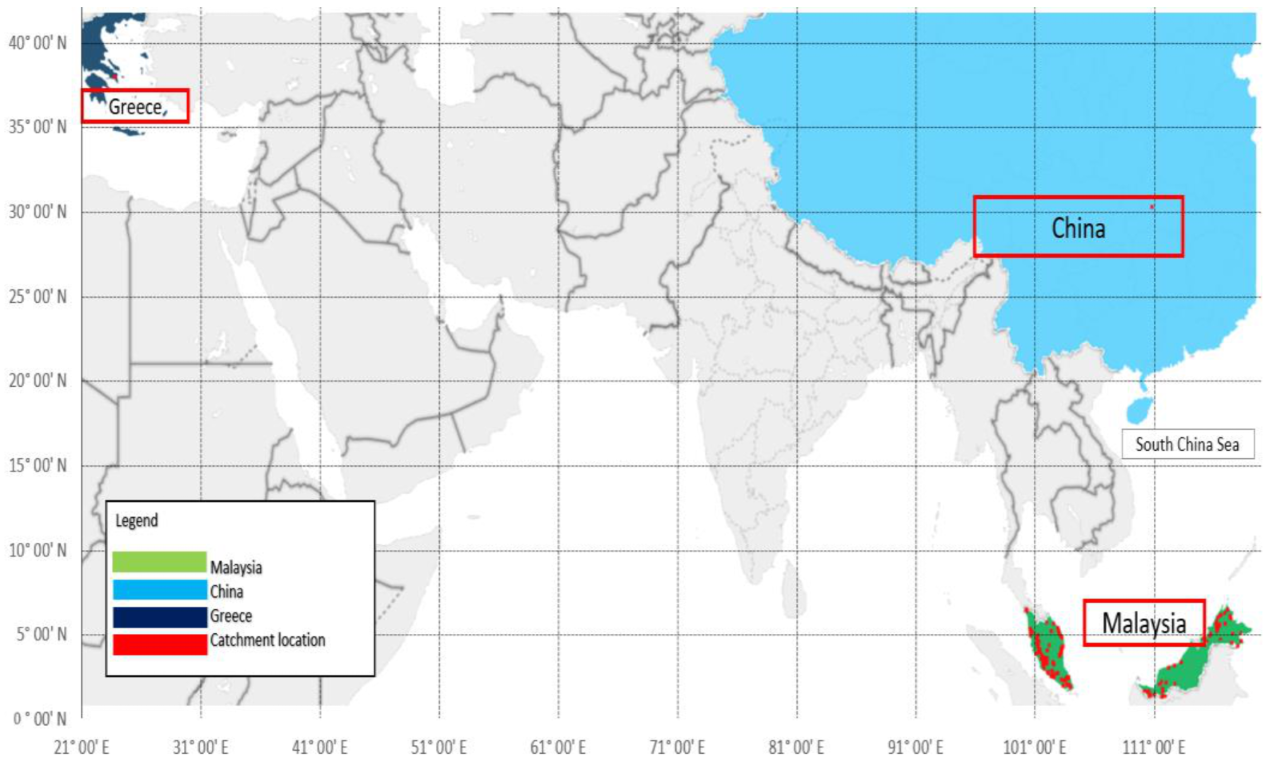
• The newly proposed power regression model (I_a = S^λ) demonstrates good runoff prediction ability at different study sites, including those in Malaysia, Greece, and China. The calibrated SCS rainfall–runoff model based on the proposed power regression model is promising for modelling the rainfall–runoff characteristics of different watersheds in different countries. The ratio of I_a to S for all study sites is mostly 5% or lower, which is in line with past worldwide study results and much lower than the value of 0.2 (20%) as suggested by the SCS.
• There is concern about the use of the original form of the SCS CN model in education, as it may teach students an oversimplified and potentially inaccurate model for predicting runoff, which could have serious consequences for fields such as water resource management, environmental science, and civil engineering. There is also concern about the widespread use of the original form of the model in educational materials, such as textbooks, software, and government agency handbooks and trainings, which may perpetuate the use of an oversimplified and potentially inaccurate model for predicting runoff.
• The proposed methodology has several limitations, including the need for a minimum sample size of at least 20 data pairs to obtain meaningful inferential results and the reliance on the bootstrap BCa method to produce confidence intervals for key variable optimization and the formulation of a new runoff predictive model. The statistical software used must also include the bootstrap BCa method as an option. There are several areas of research that have not been explored in this manuscript due to financial and time constraints. Future studies will examine the potential impacts of the proposed model on flood risk, financial losses caused by flooding, and its potential for downstream development and wider application.

References

- Danáčová, M.; Földes, G.; Labat, M.M.; Kohnová, S.; Hlavčová, K. Estimating the Effect of Deforestation on Runoff in Small Mountainous Basins in Slovakia. Water 2020, 12, 3113. [Google Scholar] [CrossRef]
- Li, Y.; Liu, C.; Zhang, D.; Liang, K.; Li, X.; Dong, G. Reduced Runoff due to Anthropogenic Intervention in the Loess Plateau, China. Water 2016, 8, 458. [Google Scholar] [CrossRef] [Green Version]
- Zhang, Y.; Xia, J.; Yu, J.; Randall, M.; Zhang, Y.; Zhao, T.; Pan, X.; Zhai, X.; Shao, Q. Simulation and Assessment of Urbanization Impacts on Runoff Metrics: Insights from Landuse Changes. J. Hydrol. 2018, 560, 247–258. [Google Scholar] [CrossRef]
- Zhai, R.; Tao, F. Contributions of Climate Change and Human Activities to Runoff Change in Seven Typical Catchments across China. Sci. Total Environ. 2017, 605–606, 219–229. [Google Scholar] [CrossRef] [PubMed]
- Li, C.; Liu, M.; Hu, Y.; Shi, T.; Qu, X.; Walter, M.T. Effects of Urbanization on Direct Runoff Characteristics in Urban Functional Zones. Sci. Total Environ. 2018, 643, 301–311. [Google Scholar] [CrossRef]
- Tedela, N.H.; McCutcheon, S.C.; Rasmussen, T.C.; Hawkins, R.H.; Swank, W.T.; Campbell, J.L.; Adams, M.B.; Jackson, C.R.; Tollner, E.W. Runoff Curve Numbers for 10 Small Forested Watersheds in the Mountains of the Eastern United States. J. Hydrol. Eng. 2012, 17, 1188–1198. [Google Scholar] [CrossRef] [Green Version]
- Ling, L.; Yusop, Z.; Yap, W.-S.; Tan, W.L.; Chow, M.F.; Ling, J.L. A Calibrated, Watershed-Specific SCS-CN Method: Application to Wangjiaqiao Watershed in the Three Gorges Area, China. Water 2019, 12, 60. [Google Scholar] [CrossRef] [Green Version]
- N.E.D.C. Engineering Hydrology Training Series. In Module 205-SCS Runoff Equation; N.E.D.C.: London, UK, 1997; Available online: https://d32ogoqmya1dw8.cloudfront.net/files/geoinformatics/steps/nrcs_module_runoff_estimation.pdf (accessed on 8 July 2022).
- Soil Conservation Service (S.C.S.). National Engineering Handbook; US Soil Conservation Service: Washington, DC, USA, 1964; Chapter 10; Section 4. Available online: https://directives.sc.egov.usda.gov/RollupViewer.aspx?hid=17092 (accessed on 10 July 2022).
- USDA; NRCS. National Engineering Handbook, Part 630 Hydrology; US Soil Conservation Service: Washington, DC, USA, 1964; Chapter 10. [Google Scholar]
- Mishra, S.K.; Babu, P.S.; Singh, V.P. SCS-CN Method Revisited. In Advances in Hydraulics and Hydrology; Water Resources Publications: Littleton, CO, USA, 2007. [Google Scholar]
- Tan, W.J.; Ling, L.; Yusop, Z.; Huang, Y.F. New Derivation Method of Region Specific Curve Number for Urban Runoff Prediction at Melana Watershed in Johor, Malaysia. In IOP Conference Series: Materials Science and Engineering; IOP Publishing: Bristol, UK, 2018; Volume 401, p. 012008. [Google Scholar] [CrossRef]
- Yuan, L.; Sinshaw, T.; Forshay, K.J. Review of Watershed-Scale Water Quality and Nonpoint Source Pollution Models. Geosciences 2020, 10, 25. [Google Scholar] [CrossRef] [Green Version]
- Hawkins, R.H.; Yu, B.; Mishra, S.K.; Singh, V.P. Another Look at SCS-CN Method. J. Hydrol. Eng. 2001, 6, 451–452. [Google Scholar] [CrossRef]
- Hawkins, R.; Ward, T.J.; Woodward, E.; van Mullem, J.A. Continuing Evolution of Rainfall-Runoff and the Curve Number Precedent. In Proceedings of the 2nd Joint Federal Interagency Conference, Las Vegas, NV, USA, 27 June–1 July 2010; pp. 1–12. [Google Scholar]
- Tan, W.J.; Ling, L.; Yusop, Z.; Huang, Y.F. Claim Assessment of a Rainfall Runoff Model with Bootstrap. In Proceedings of the Third International Conference on Computing, Mathematics and Statistics (iCMS2017), Langkawi, Malaysia, 7–8 November 2017; Springer Nature: Singapore, 2019. [Google Scholar]
- Hawkins, R.H.; Khojeini, A.V. Initial Abstraction and Loss in the Curve Number Method. Hydrology and Water Resources in Arizona and the Southwest 2000, 30, 29–35. [Google Scholar]
- DID. Hydrological Procedure 27 Design Flood Hydrograph Estimation for Rural Catchments in Malaysia; JPS, DID: Kuala Lumpur, 2010. Available online: https://www.water.gov.my/jps/resources/PDF/Hydrology%20Publication/Hydrological_Procedure_No_27_(HP_27).pdf (accessed on 5 August 2022).
- DID. Hydrological Procedure 11 Design Flood Hydrograph Estimation for Rural Catchments in Malaysia; JPS, DID: Kuala Lumpur, 2018. Available online: http://h2o.water.gov.my/man_hp1/HP11.pdf (accessed on 20 July 2022).
- Abustan, I.; Sulaiman, A.H.; Wahid, N.A.; Baharudin, F. Determination of Rainfall-Runoff Characteristics in An Urban Area: Sungai Kerayong Catchment, Kuala Lumpur. In Proceedings of the 11th International Conference on Urban Drainage, Palermo, Italy, 23–26 September 2018; Springer International Publishing: New York, NY, USA, 2018. [Google Scholar]
- Ling, L.; Chow, M.F.; Tan, W.L.; Tan, W.J.; Tan, C.Y.; Yusop, Z. New Regional-Specific Urban Runoff Prediction Model of Sungai Kayu Ara Catchment in Malaysia. In Lecture Notes in Civil Engineering; Springer Nature: Singapore, 2020; Volume 59, pp. 161–168. [Google Scholar]
- Baltas, E.A.; Dervos, N.A.; Mimikou, M.A. Technical Note: Determination of the SCS Initial Abstraction Ratio in an Experimental Watershed in Greece. Hydrol. Earth Syst. Sci. 2007, 11, 1825–1829. [Google Scholar] [CrossRef] [Green Version]
- Efron, B.; Tibshirani, R.J. An Introduction to the Bootstrap; Chapman and Hall/CRC: New York, NY, USA, 1993; ISBN 978-0-412-04231-7. [Google Scholar]
- Davison, A.C. Cambridge Series in Statistical and Probabilistic; Cambridge University Press: New York, NY, USA, 2003; ISBN 978-0-511-67299-6. [Google Scholar]
- Efron, B. Large-Scale Inference: Empirical Bayes Methods for Estimation, Testing, and Prediction; Cambridge University Press: New York, NY, USA, 2013; ISBN 978-1-107-61967-8. [Google Scholar]
- Rochowicz, J.A.J. Bootstrapping Analysis, Inferential Statistics and EXCEL. Spredsheets Educ. (Ejsie) 2010, 4, 1–23. [Google Scholar]
- Moriasi, D.N.; Arnold, J.G.; van Liew, M.W.; Bingner, R.L.; Harmel, R.D.; Veith, T.L. Model Evaluation Guidelines for Systematic Quantification of Accuracy in Watershed Simulations. Trans. ASABE 2007, 50, 885–900. [Google Scholar] [CrossRef]
- Nash, J.E.; Sutcliffe, J.V. River Flow Forecasting through Conceptual Models Part I—A Discussion of Principles. J. Hydrol. 1970, 10, 282–290. [Google Scholar] [CrossRef]
- Ling, L.; Yusop, Z.; Ling, J.L. Statistical and Type II Error Assessment of a Runoff Predictive Model in Peninsula Malaysia. Mathematics 2021, 9, 812. [Google Scholar] [CrossRef]
- Knoben, W.J.M.; Freer, J.E.; Woods, R.A. Technical Note: Inherent Benchmark or Not? Comparing Nash—Sutcliffe and Kling—Gupta Efficiency Scores. Hydrol. Earth Syst. Sci. 2019, 23, 4323–4331. [Google Scholar] [CrossRef] [Green Version]
- Miles, J. R Squared, Adjusted R Squared. In Wiley StatsRef: Statistics Reference Online; Wiley: Hoboken, NJ, USA, 2014. [Google Scholar]
- Hawkins, R.H.; Theurer, F.D.; Rezaeianzadeh, M. Understanding the Basis of the Curve Number Method for Watershed Models and TMDLs. J. Hydrol. Eng. 2019, 24, 06019003. [Google Scholar] [CrossRef]
- Ling, L.; Yusop, Z. Derivation of Region-Specific Curve Number for an Improved Runoff Prediction. In Improving Flood Management, Prediction and Monitoring: Case Studies in Asia; Community, Environment and Disaster Risk Management; Emerald Publishing Limited: Bingley, UK, 2018; Volume 20, pp. 37–48. ISBN 978-1-78756-552-4. [Google Scholar]
- Ling, L.; Yusop, Z.; Chow, M.F. Urban Flood Depth Estimate with a New Calibrated Curve Number Runoff Prediction Model. IEEE Access 2020, 8, 10915–10923. [Google Scholar] [CrossRef]
- Mosavi, A.; Ozturk, P.; Chau, K. Flood Prediction Using Machine Learning Models: Literature Review. Water 2018, 10, 1536. [Google Scholar] [CrossRef] [Green Version]
- Pinos, J.; Quesada-Román, A. Flood Risk-Related Research Trends in Latin America and the Caribbean. Water 2021, 14, 10. [Google Scholar] [CrossRef]
- Fu, M.; Fan, T.; Ding, Z.; Salih, S.Q.; Al-Ansari, N.; Yaseen, Z.M. Deep Learning Data-Intelligence Model Based on Adjusted Forecasting Window Scale: Application in Daily Streamflow Simulation. IEEE Access 2020, 8, 32632–32651. [Google Scholar] [CrossRef]
- Kaya, C.M.; Tayfur, G.; Gungor, O. Predicting Flood Plain Inundation for Natural Channels Having No Upstream Gauged Stations. J. Water Clim. Change 2019, 10, 360–372. [Google Scholar] [CrossRef] [Green Version]