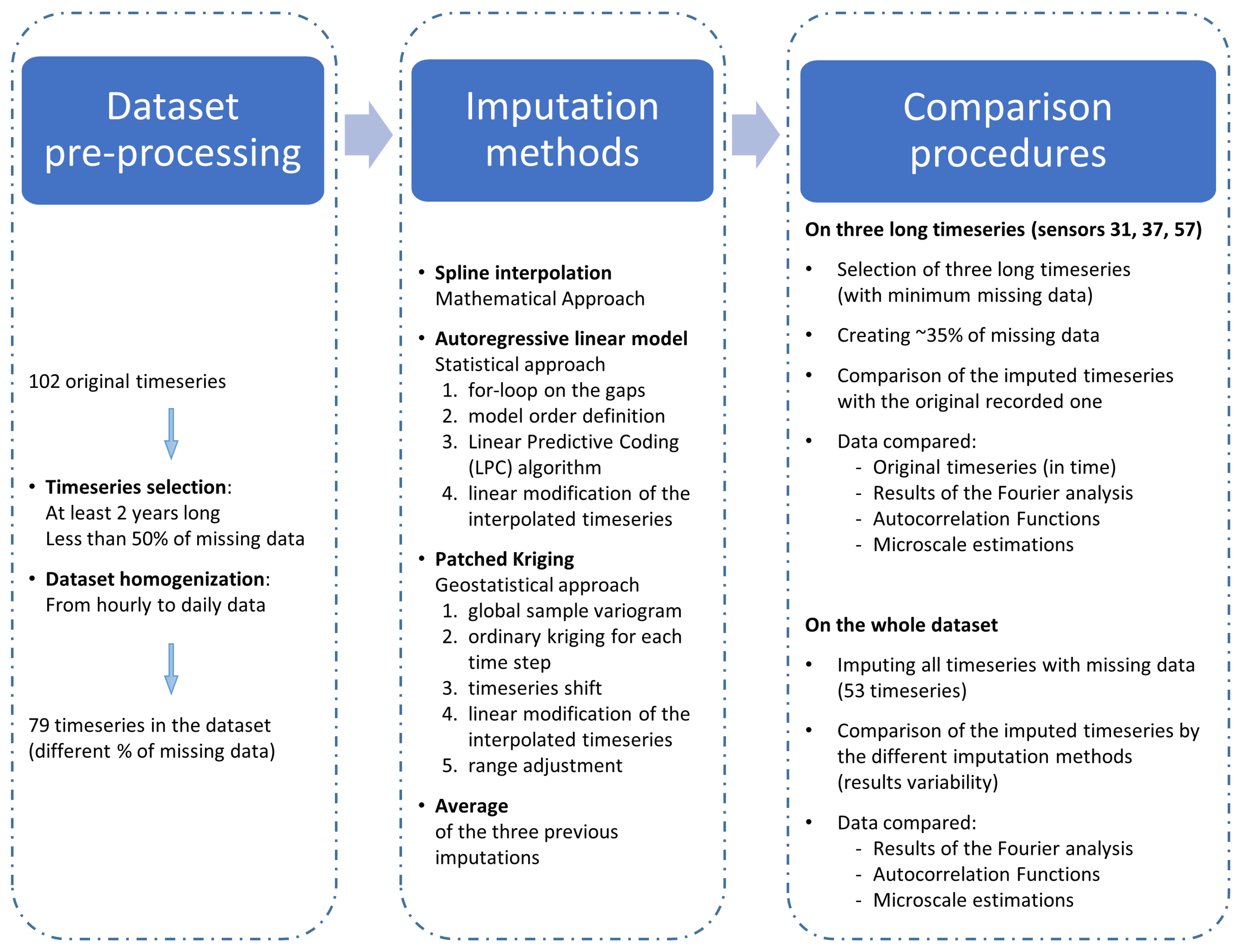
2.3. Imputation Methods
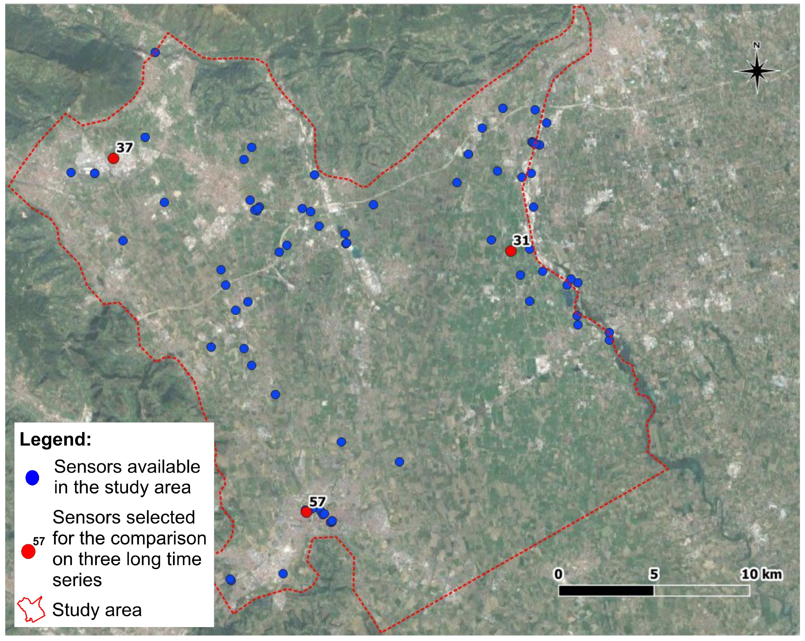
The study applied three existing imputation methods, described in this section, adapted to the treatment of groundwater level timeseries. The first two, namely the cubic spline interpolation and the autoregressive linear model, focus on a single timeseries, while the patched kriging exploits the spatial correlation structure shown by the measured groundwater levels. Thus, the applied methods test the applicability, and the quality of the resulting fit, of both time and spatial imputation. In order to describe and to better comprehend the adjustments needed to the selected imputation methods, the resulting interpolated timeseries are reported and commented for three complete long samples (sensors 31, 37, and 57, shown in
Figure 2). The same timeseries were used for comparative purposes when gaps were artificially created by removing recorded data.
The cubic spline interpolation (CS) is a mathematical interpolation, which, based on the information of the timeseries alone, applies a piecewise cubic polynomial approximating function to obtain a smooth approximation. As explained by [
51], the piecewise cubic interpolators
f handle data points
with
. In each subinterval
, the interpolating function
f coincides with a polynomial
of order 4 that satisfies the following conditions:
where
are defined as “free slopes”. Therefore, the interpolating
f agrees with the data points, it is continuous, and it has a continuous first derivative on the interval
. There exist different piecewise interpolation schemes, depending on the choice of the slopes evaluation: the applied CS interpolation adds the condition where the second derivative of the interpolating function
f is also continuous; thus,
f is twice continuously differentiable:
. In this analysis, the interpolation is carried out by calling the
spline function in MATLAB.
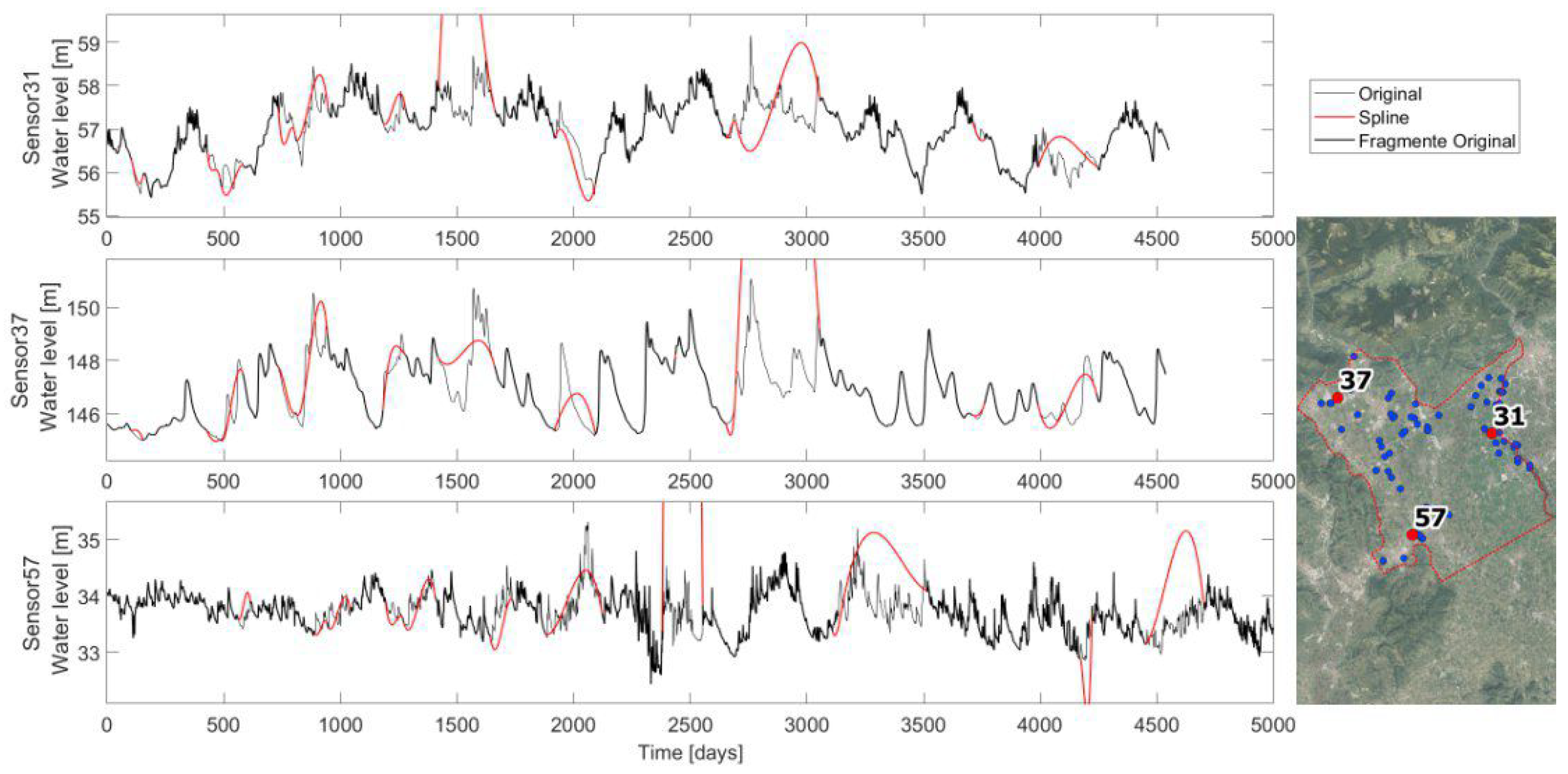
The resulting CS interpolations for sensors 31, 37, and 57 are reported in
Figure 3. As is noticeable, sometimes the spline interpolation achieves maximums and minimums that are never observed by the recorded timeseries. If this happens, the CS is not considered as a plausible imputation method. The exact applied conditions are:
The minimum spline value must be greater than the recorded minimum less one quarter of the recorded range;
The maximum spline value must be smaller than the recorded maximum plus one quarter of the recorded range.
The autoregressive linear model (AR) is a statistical approach which, based on the information of the timeseries alone, aims to predict a realization of an underlying random processes based on past observations. Specifically, the estimated present value at
k is considered to be approximated by a linear combination of
n past observations. The number of past values
n used by the procedure is the model order, and it intends to represent the process memory. The coefficients selected for the linear combination are constant parameters of the model that are therefore considered to be invariant in time.
In order to apply an AR model to a timeseries, it is required to first identify the appropriate order, and to estimate the coefficients by using the Linear Predictive Coding (LPC) algorithm—
lpc function in MATLAB. In this study, the code used is the one described by [
35], which has been adapted to this specific groundwater analysis. The code’s specifications are in [
52]. What follows outlines the general procedure and the changes that are implemented. The basic assumptions are also discussed.
The AR procedure starts from a simple linear interpolation of all intervals of missing values shorter than 5 days and from a for-loop on the remaining gaps in the timeseries. For each gap, the model order is assumed to be equal to three-quarters of the prior known record length in order to use most of the available information. The known sequence is subtracted by its own mean, and the coefficients are estimated with the LPC algorithm, considering the modified timeseries. The forecast series imputing the gap is estimated using the identified linear combination, and by adding again the previously subtracted mean. Sometimes, the AR forecasted series ends () with a value that considerably diverges from the first known value after the gap , thus creating an unrealistic step-shaped trend. This happens as this forecasting procedure does not consider the available knowledge of the recorded sequence after the gap. In order to adjust such a final step, the interpolated timeseries is linearly modified within the gap in order to obtain a final forecasted value coinciding with the first value of the following known record: i.e., the timeseries S is corrected by summing up a linearly increasing factor that ranges from 0 in the first unknown value (), and in the last unknown value (). The timeseries is then updated with the interpolated sequence and the following gap of the for-loop will consider all previous values as being known and usable for its own interpolation. This for-loop applies only if the previous knowledge covers a sequence that is longer than 30 days, otherwise the information is too poor and a spline interpolation is applied for the first gaps, up to the satisfaction of the condition.
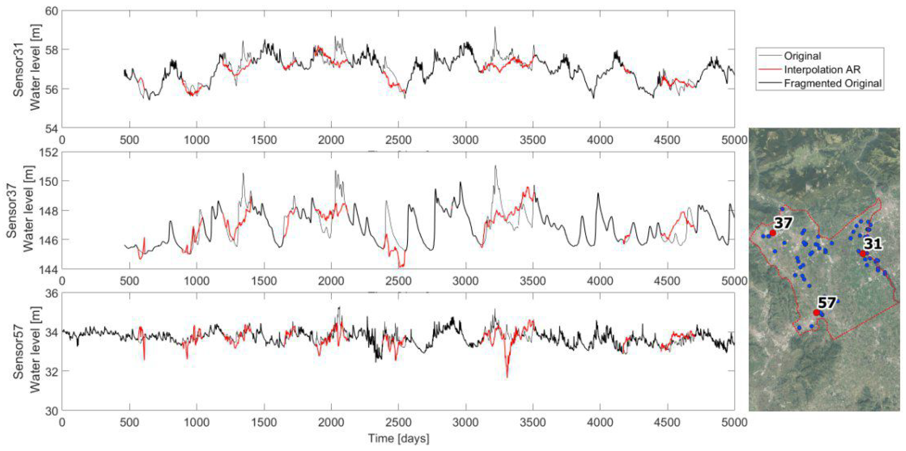
The interpolation is applied to the three long timeseries previously identified, and
Figure 4 reports the resulting interpolations. Observing the graphs, it is noticeable how the interpolation can mimic the local hydrogeological behavior, even if sometimes it creates unreal minimums and peaks. This is due to the statistical approach that lacks hydrological knowledge and guidance.
Differently from the previous methods, the patched kriging (PK) is a geostatistical approach that takes advantage of the spatial information of the groundwater level. It has been originally proposed and implemented by [
34] in order to deal with uneven and fragmented rainfall records that are useful for the statistical assessment of extremes. The method considers each measurement as a 3D point
, and for each timestep, a spatial interpolation in the whole domain is carried out. This way, missing values in the timeseries can be evaluated owing to the concomitant information in other measurement points, extracting information from timeseries recorded nearby in space. To the authors’ knowledge, this method has been never applied to impute groundwater level timeseries. This technique evaluates the parameter value also in unmeasured points, but it is not a result of interest in this study.
Each measurement is considered as a 3D point
for each time instant the hydraulic data are spatially interpolated. The method applied by [
34] and by this study is the ordinary kriging. All details regarding kriging are extensively available in the geostatistical literature, e.g., [
53]. Differently from the original study, the here applied PK method does not correct the data for elevation effects. The current analysis directly evaluates the spatial dependence of measured records by estimating a sample variogram as:
where
L is the lag distance,
and
are observations lagged by a distance
L, and
is the number of pairs separated by lag
L. As in [
34], for each timestep, the sample variogram is evaluated by using Equation (
4), and the global sample variogram is estimated as a weighted average of these. The weights are defined as the number of measuring points in each timestep. Then, the theoretical variogram is estimated with the exponential form best fitting the global sample variogram. The exponential model has been simply selected as first attempt, given the preliminary phase of this comparative study. This variogram model needs the definition of the nugget and the number of the considered nearest points: the nugget effect is neglected, and therefore, the measured values are preserved, while the latter parameter is arbitrary and there are different objects to look at in order to define it. It depends on the desired variability scale: few neighbors for identifying a small scale, and up to the whole sample if the small scale is not required and if a shorter computational time is desired. Ref. [
54] suggest a number of between 10 and 20, even if this number should depend on the range of the evaluated variogram. In this study, as well as in [
34], given that for each timestep the number and the spatial distribution of recording sensors varies, the variogram range has been used as a first hint for selecting the number of nearest points. Given the sensors’ spatial distribution within the domain and the estimated range, the algorithm always considers the 10 closest sensors for the kriging interpolation. In this manner, a minimum amount of information is also guaranteed also in areas with a lower density of sensors.
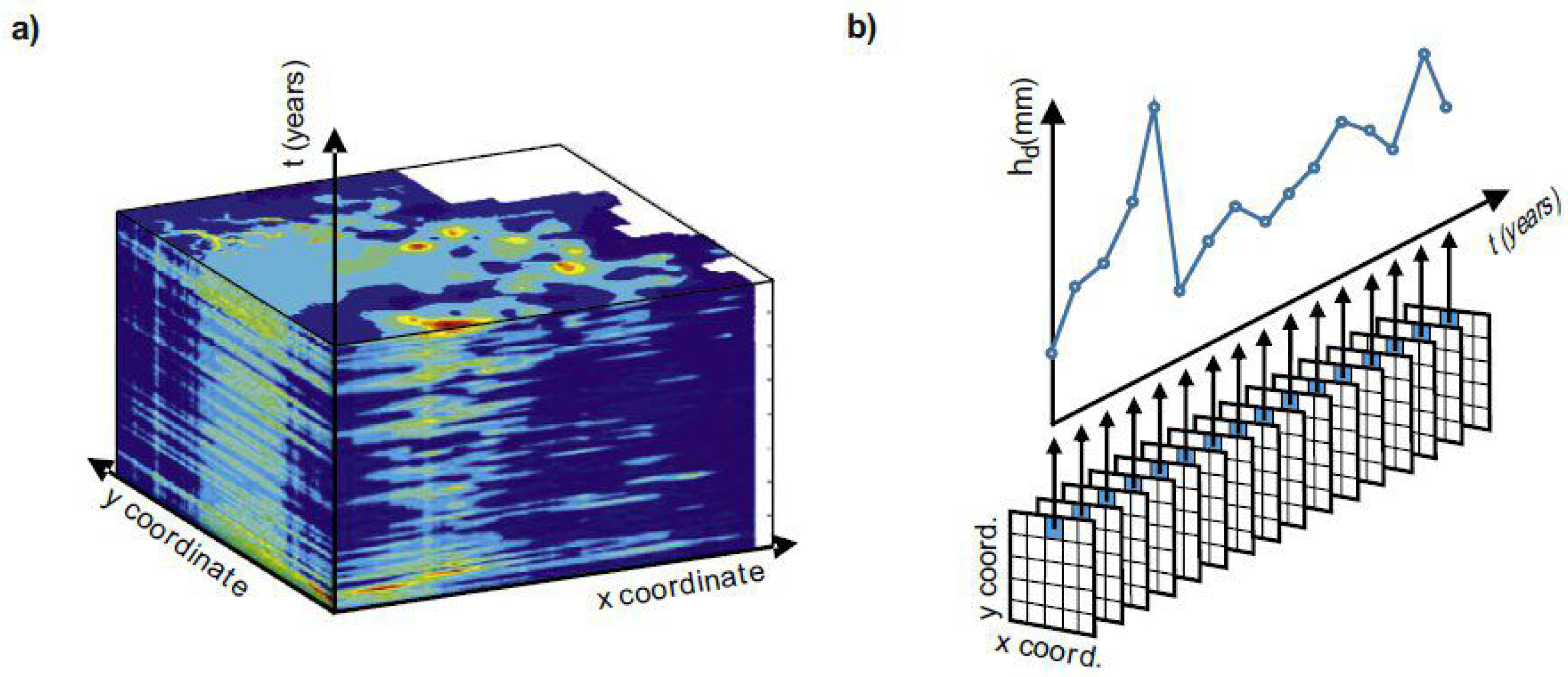
After the space interpolation and the creation of a map for each timestep with a space resolution of 25 m × 25 m, complete timeseries are extracted for each sensor location: i.e., given the space coordinates of a sensor
, the complete series in the
t axis is extracted from all maps, see
Figure 5.
Moreover, the interpolated timeseries have to be further adjusted with respect to the procedure of [
34]. The Extracted timeseries coincides with the recorded one when data are available, but it can be offset in interpolated gaps as the water level is driven by surrounding points that could have different average elevations. Nevertheless, the oscillations of the neighboring timeseries are significant information to be extracted by the spatial interpolation. Therefore, the timeseries are shifted in order to have the first interpolated value of the gap
be coincident with the last known value
(
). Moreover, looking at the shifted timeseries, often it shows a step between the last shifted interpolated value
and the first recorded value after the gap
. This step can be upward, showing a hydrogeological peak, or downward, which is less realistic for a descending water level. Indeed, the ascending side of the hydrogeological peak can be very steep, while the descending one has always a slighter slope. A correction is applied only for the descendant phase (
) linearly modifying the interpolated series and making the two points coincide
.
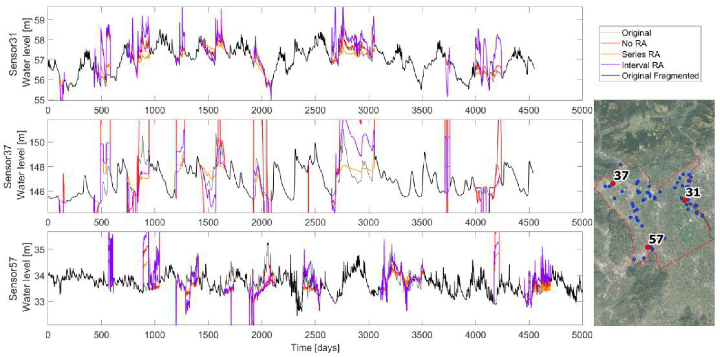
Another needed adjustment is made with regard to the oscillations range. Depending on the hydrogeological local connections, between the recording sensors, the oscillations range could be very different. In order to define which range adjustment (RA) to use, three possibilities are investigated and compared on imputing the three complete long timeseries. The three options are: (i) no range adjustment; (ii) series arrangement, meaning that the whole interpolated timeseries is proportionate in order to have the same range as the original fragmented timeseries; and (iii) interval arrangement, by proportioning the interpolated timeseries on each gap with the original record. Looking at the results comparison in
Figure 6, different observations arise. In sensor 31, the PK works well on the reproduction of the real timeseries, and even with no range adjustment, the reconstructed timeseries well fits the reality in almost all gaps. This is probably due to the availability of many nearby surrounding points that well guide the imputation method. On the contrary, sensor 37 is not well reproduced and a range adjustment is necessary. The interval adjustment has water level oscillations that are close to the recorded ones, but they are shifted. The series adjustment is well located on average, the problem is that the fluctuations are softened. Finally, sensor 57 is similarly interpolated by the different range adjustments. In general, the interval RA has the tendency to enhance fluctuations, and not adjusted RA is sometimes the best option (sensor 31), even if occasionally it is completely out of the series range (sensor 37), while the series RA seems to be the safest option, even if it tends to soften the peaks. The best RA option is chosen by comparing the mean percentage daily errors, defined as the Euclidean distance divided by the total missing values of the series, and scaled based on the oscillations range:
where
and
are the interpolated and original timeseries,
is the total number of missing values, and
r is the recorded range of the original timeseries. The error is evaluated for each sensor and for each interpolation.
Table 1 highlights as the interpolation with a series range of adjustment that better fits the original timeseries: it is always the minimum error. This RA is therefore chosen for the PK imputation method. Additionally, these results (particularly in the imputation of the timeseries of sensor 37) clearly show how sometimes the PK technique is step-shaped and where the applied shift procedure is not enough. This is probably because the imputed timeseries does not have so many recording sensors nearby, hence, it is sensitive to the activation and deactivation of the few surrounding points.
The last interpolation is the average of all previous imputation methods. Note that if the spline interpolation has been removed because it failed to respect the aforementioned range conditions, the average is only between the autoregressive linear model and the patched kriging methods.
2.4. Comparing Procedures and Applied Statistical Analyses
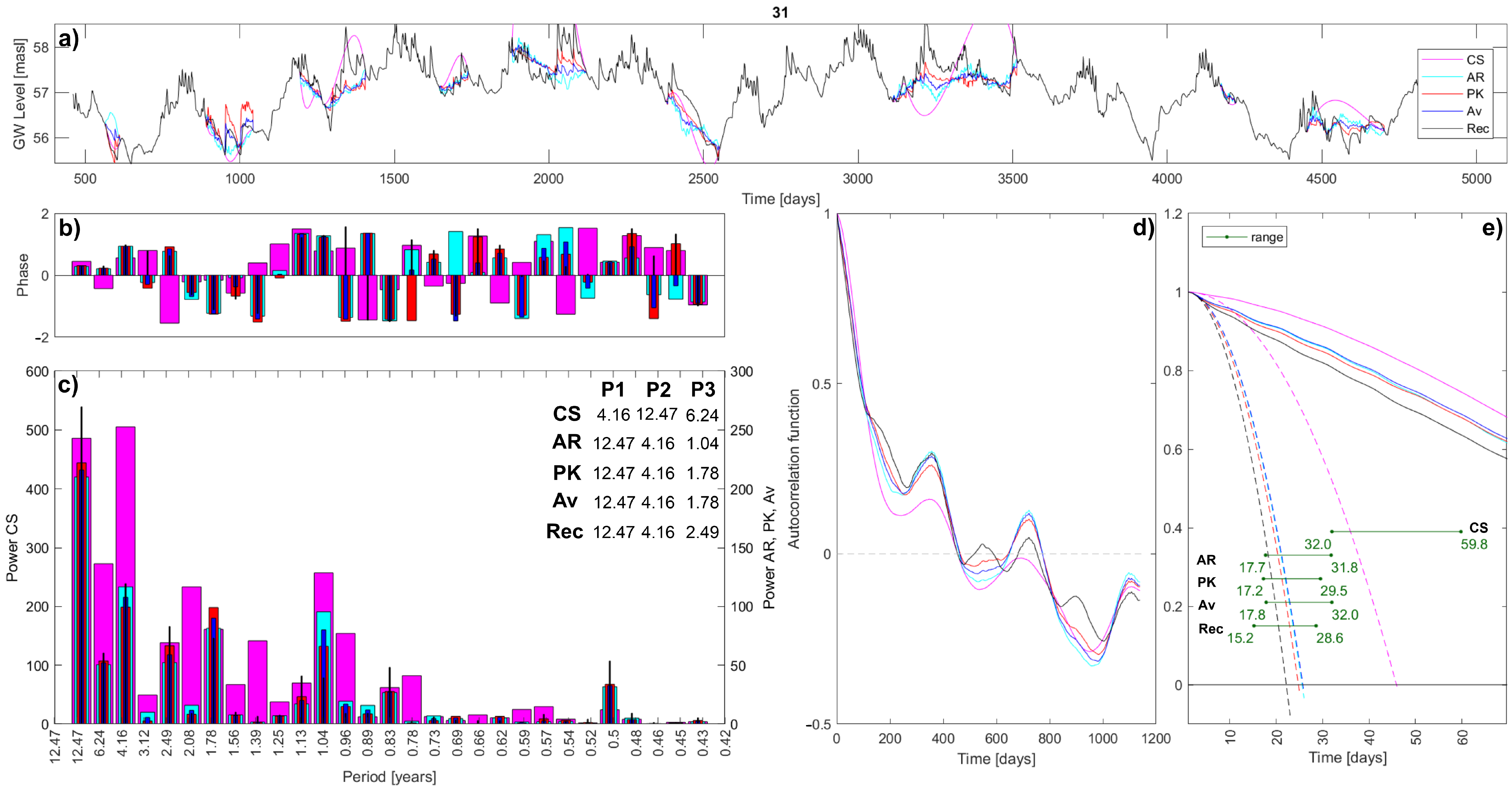
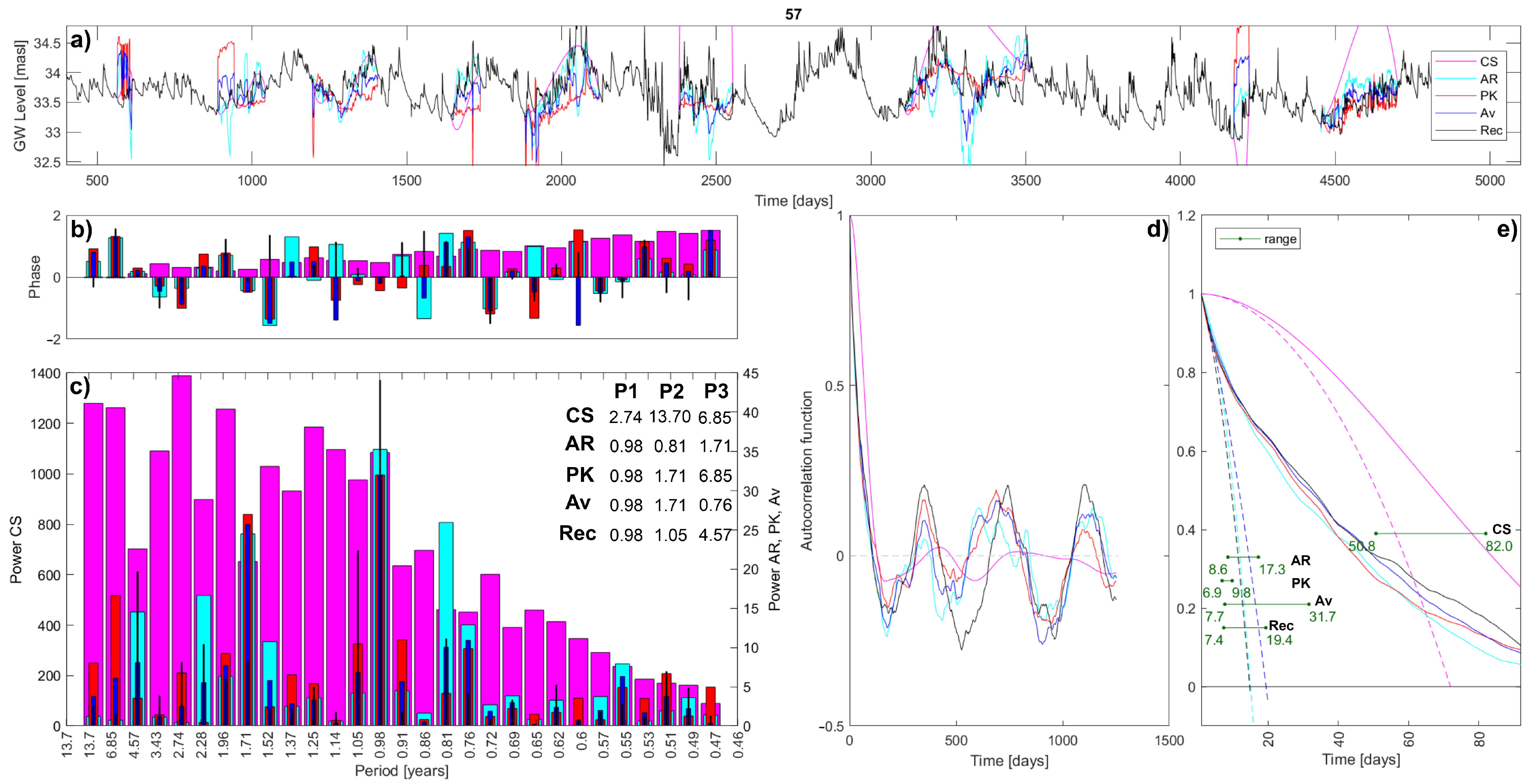
For an easy understanding of the imputation methods performances, the first procedure compares interpolations with true timeseries: the comparison in time domain that returns an immediate feeling of the interpolation’s goodness is easy to comprehend and evaluate, then statistical analyses are applied to see how sensitive these analyses are to the chosen imputation method. This comparison with the true timeseries is possible only for a few timeseries of the dataset: three series have been identified to be at least 12 years long, with less than
of missing values, and located far away from each other in order to not bias the analysis. The identified timeseries are 31, 37, and 57, the locations of which are shown in
Figure 2. The three timeseries have been fragmented in MATLAB by randomly creating 12 gaps, applying the functions
randfixedsum e
randi. The fragmentation procedure has been guided by removing
of the shortest timeseries (1608 values), and it created variably long gaps ranging from 45 to 356 days.
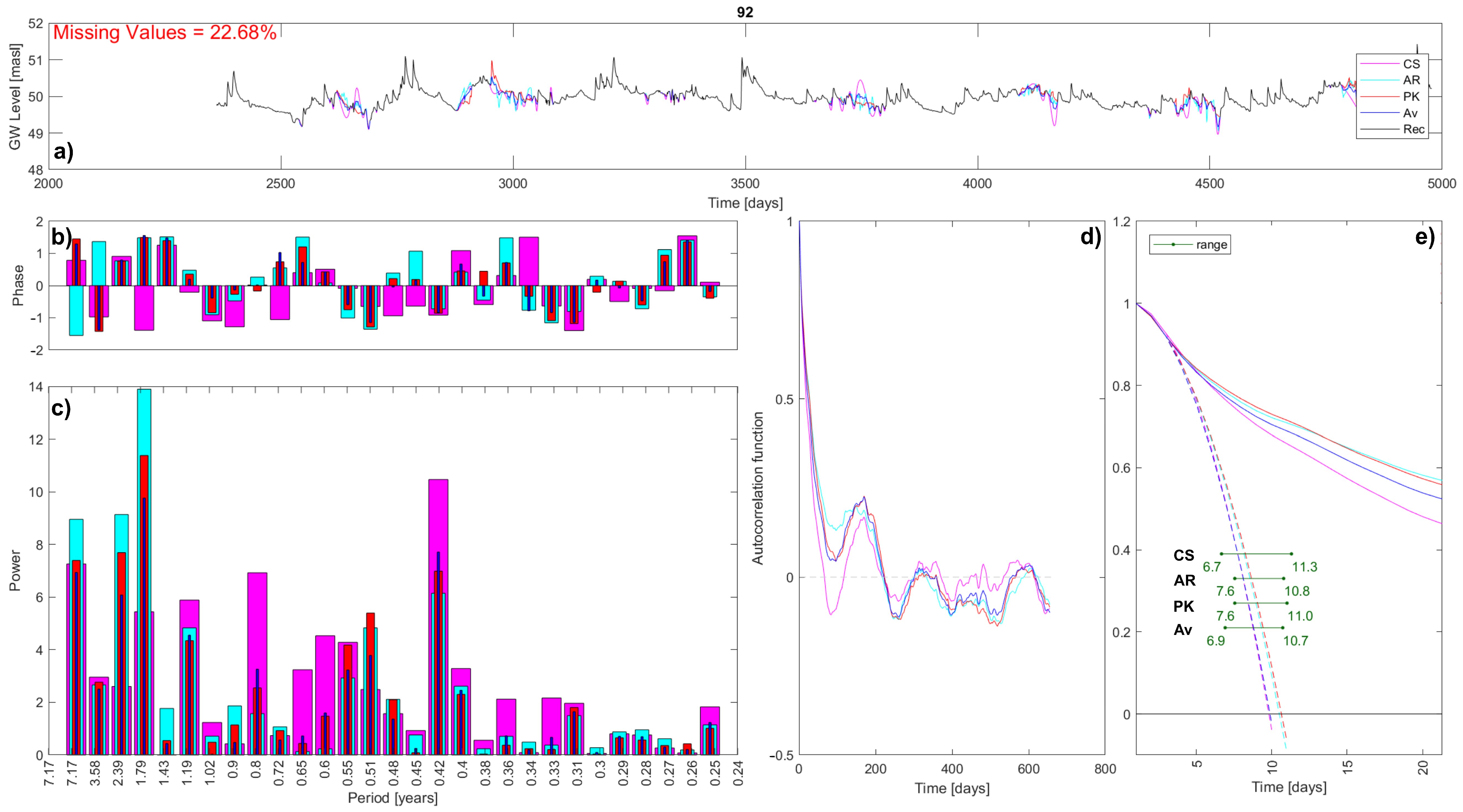
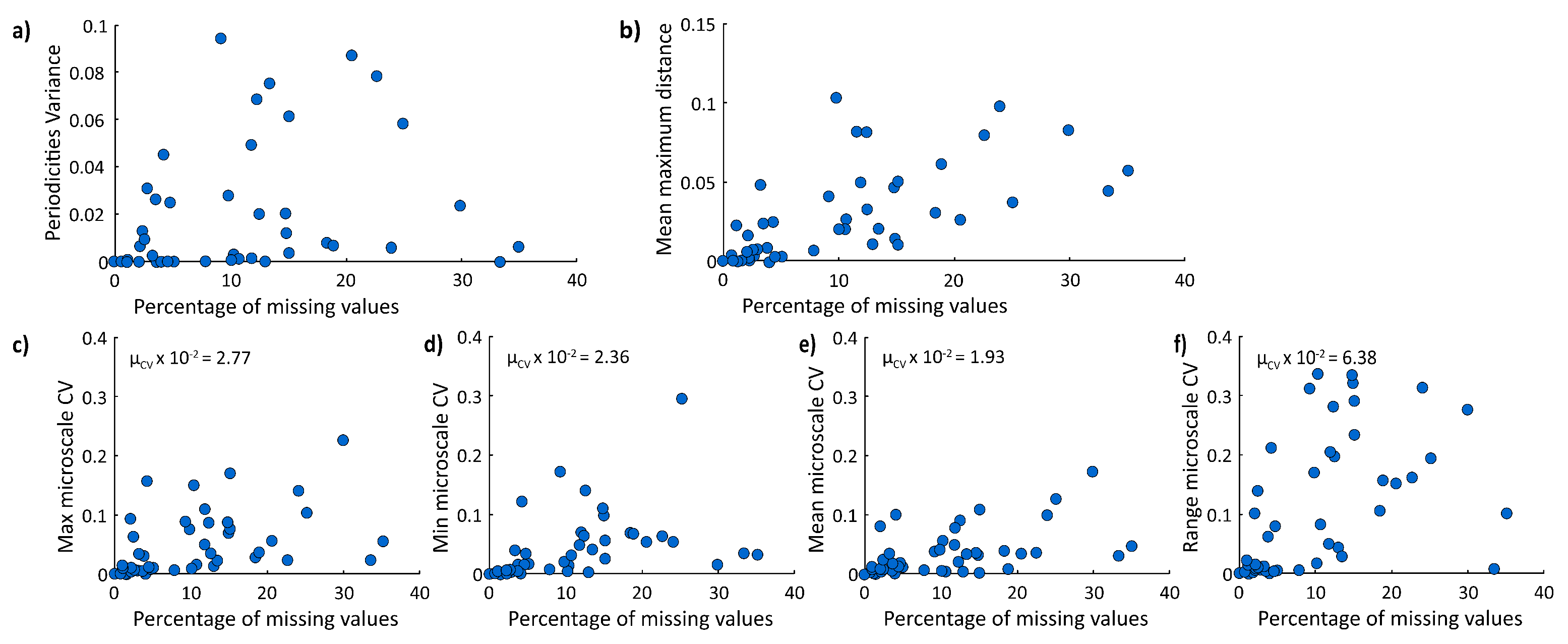
The second procedure aims to compare the results of the imputation methods on the whole dataset, using all of the available timeseries to evaluate how much of the method is affecting the results of some statistical analyses. This returns an idea of the importance of correctly selecting the imputation method, even if the comparison with the reality is not possible. It is substantially a sensitivity analysis.
As a comparison of imputations, both procedures apply and compare the results of three statistical analyses, with the following being briefly described: Fourier analysis, autocorrelation, and microscale. The Fourier analysis provides a different view of timeseries because it analyses them in the frequency domain [
55]. Its main result is the power spectrum that points out timeseries periodicities, which are usually not easily recognizable in the time domain. This result is often interesting for hydrogeological studies, as the main hydraulic periodicities depend on the most relevant hydraulic drivers affecting the site. The Discrete Fourier transform is carried out to move from the time to the frequency domain by applying the Fast Fourier Transform algorithm-
fft function in MATLAB. The second statistical analysis is the evaluation of the autocorrelation function that defines the correlation (Pearson coefficient [
53]) of a signal with a delayed copy of itself as a function of the time lag
k. This analysis is usually useful for having insights on signal persistence and periodicity. The sample autocorrelation function (ACF) is defined by applying the
autocorr function in MATLAB. The final analysis is the definition of an integral scale parameter, the microscale. It represents the time interval in which values are perfectly correlated, and it is an indication of the series memory and fluctuations rapidity. There are three ways to evaluate it:


 ,
, 


