Analysis and Processing of the COSMO-SkyMed Second Generation Images of the 2022 Marche (Central Italy) Flood

Abstract

The use of SAR data for flood mapping is well established. However, the problem of the missed detection of rapidly evolving floods remains. Recently, the Italian Space Agency deployed the COSMO-SkyMed Second Generation (CSG) constellation, with an on-demand capability that makes it possible to reduce the number of missed floods. However, for on-demand SAR acquisitions, pre-flood images are generally not available, and change-detection methods, commonly adopted for flood mapping using SAR, cannot be applied. This study focused on the high-resolution CSG images of a flood that occurred in central Italy. An accurate analysis of the radar responses of the different targets included in the scenes observed by GSG was performed. Then, a methodology to detect floods using high-resolution single SAR images was developed. The methodology was based on image segmentation and fuzzy logic. Image segmentation allowed us to analyze homogeneous areas in the CSG images. Fuzzy logic was used to integrate the SAR data with ancillary information that was useful when change-detection methods could not be applied. A comparison with the maps produced by the Copernicus Emergency Service, using high-resolution optical images, demonstrated the reliability of the methodology.

1. Introduction

Floods are the most frequent weather disasters in the world, as well as the costliest in terms of economic losses. They have a strong impact on infrastructure and human health because their consequences include casualties, the loss of housing, and the destruction of crops. Synthetic aperture radar (SAR) images are particularly useful for flood mapping (e.g., [1]) because SAR systems provide data both day and night, in almost any meteorological conditions. Moreover, calm water is easily detected in SAR images because it has a distinguishable radar signature characterized by a low radar return (backscattering coefficient σ⁰).

The low σ⁰ from calm water is because most of the incident radar energy is scattered by the smooth surface of the water, in the specular direction. This is why water surfaces appear dark in SAR images. Conversely, rough, non-flooded terrain scatters the radar signal in many different directions, resulting in a higher σ⁰ and brighter image tones [2]. However, other smooth surfaces, such as asphalt, produce a low σ⁰. Moreover, the areas affected by shadow appear extremely dark. Change detection is very useful to distinguish floodwater from permanent water, as well as to limit the number of false positives potentially caused by other targets that produce a low backscatter. Change detection has been used not only to map open water but also to detect floodwater in agricultural and urban areas [3,4,5,6,7].

The Sentinel-1 (S-1) constellation of two satellites has proven to be very useful for flood mapping through change detection using pairwise SAR acquisitions (e.g., [8]). Over land, the S-1 data, which are systematically available in the interferometric wide swath (IWS) mode, guarantee the availability of pre-flood images acquired with the same configuration geometry of the flood images. Therefore, the S-1 constellation represents a significant opportunity to provide emergency managers with timely flood-mapping service. The systems providing continuous and near real-time monitoring of flood events at national (e.g., [9,10,11]) or even global scales (e.g., the Global Flood Monitoring Product of the Copernicus Emergency Management Service [12]) have been designed based on S1 data.

The timeliness of the availability of the SAR data is a fundamental requirement to promptly provide a synoptic overview of the extent of a flood. After the Sentinel-1B launch (April 2016), the S-1 constellation was able to image the planet with a maximum frequency of every six days (corresponding to the exact repetition cycle). Unfortunately, in December 2021, S-1B experienced an anomaly, which made it unable to deliver radar data. Months later, the end of the S-1B mission was announced. Therefore, until the launch of the S-1C (expected in 2023), the S1 repeat cycle is 12 days. This time interval may be enough to monitor large-scale and long-term flood events, which can last weeks and even months. However, in small basins, floods are typically characterized by water rapidly receding over a short duration (even less than one day). In this case, SAR sensors offering a higher temporal resolution or on-demand capabilities are needed to limit the number of missed events.

The COSMO-SkyMed (CSK) constellation of four satellites, hosting an X-band SAR, has demonstrated a good suitability for rapid flood mapping ([13,14,15,16,17]) due to its capability in meeting real-time user requests (i.e., the ability to deliver an image product required by an end-user in a timely manner). Furthermore, the CSK operates as an on-demand earth observation system to ensure the timely provision of data. The COSMO-SkyMed Second Generation (CSG) aims to provide service continuity for the first generation while improving performance, functionality, and system services for the user community. In particular, to improve the CSG’s on-demand capability with respect to the CSK, the CSG has new and improved features, such as better response time, last-minute planning, near-real-time data delivery, and on-demand area coverage [18].

The features mentioned above make the CSG a fundamental source of data for inundations characterized by water rapidly receding. However, the on-demand capabilities of the satellite imply that the availability of pre-flood images acquired with the same configuration in terms of geometry of the flood image is not guaranteed, and thus, change detection cannot be applied.

The recent deployment of the CSG constellation and the infeasibility of the application of change detection methods has resulted in, to the best of our knowledge, no published papers concerning flood mapping using CSG data. Recently, CSG images have been used to map the severe flood that affected the Marche region in central Italy in September 2022. In particular, two images were acquired in the dual polarization and spotlight modes to observe two rural areas upstream from the city of Senigallia (one of the cities most affected by the flooding).

This paper presents the major outcomes of a detailed analysis of the CSG images of the Marche flood. We selected fields as samples to represent different types of targets, such as rough and smooth soils, vegetated fields, open water, and flooded vegetation, and the interpretation of radar response for these samples enabled us to design a methodology for flood mapping based on a single, high-resolution SAR image, for which we integrated ISODATA clustering [19] and fuzzy logic [20]. The flood mapping procedure is described in detail, and to evaluate its reliability, this paper also presents the results of the comparison between the flood maps generated by applying the proposed methodology and the maps produced by the Copernicus Emergency Service using optical images.

2. Materials and Methods

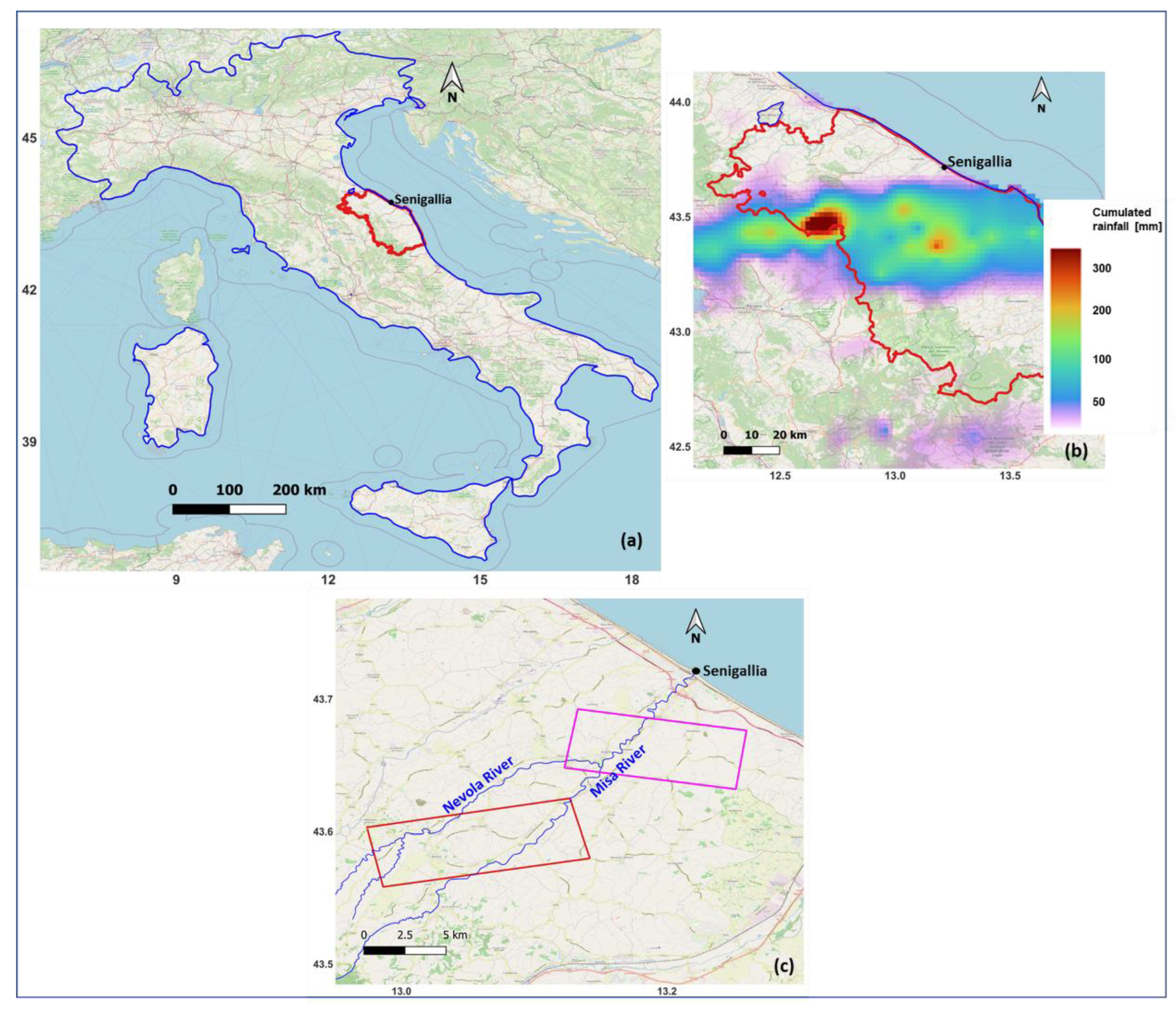
2.1. The 2022 Marche Flood

On the afternoon of 15 September 2022, an intense, auto-regenerating storm system persisted for several hours over the northern area of the Marche region (see Figure 1a), causing torrential rainfall. Cumulative rainfall values higher than 300 mm in a few hours (Figure 1b) with peaks of up to 40 mm over 15 min were recorded. This triggered the overflows of several waterways, especially the Misa River and the Nevola River (Figure 1c), resulting in a disastrous flood that killed at least 10 people. Many fields were submerged, causing severe damage to the agriculture. Furthermore, one of Italy’s worst droughts in decades, which occurred during the previous summer (2022), made the territory prone to floods. The soil was very dry and, therefore, less capable of absorbing water.

The on-demand capability of the CSG was exploited to map the two areas upstream from the city of Senigallia shown in Figure 1c.

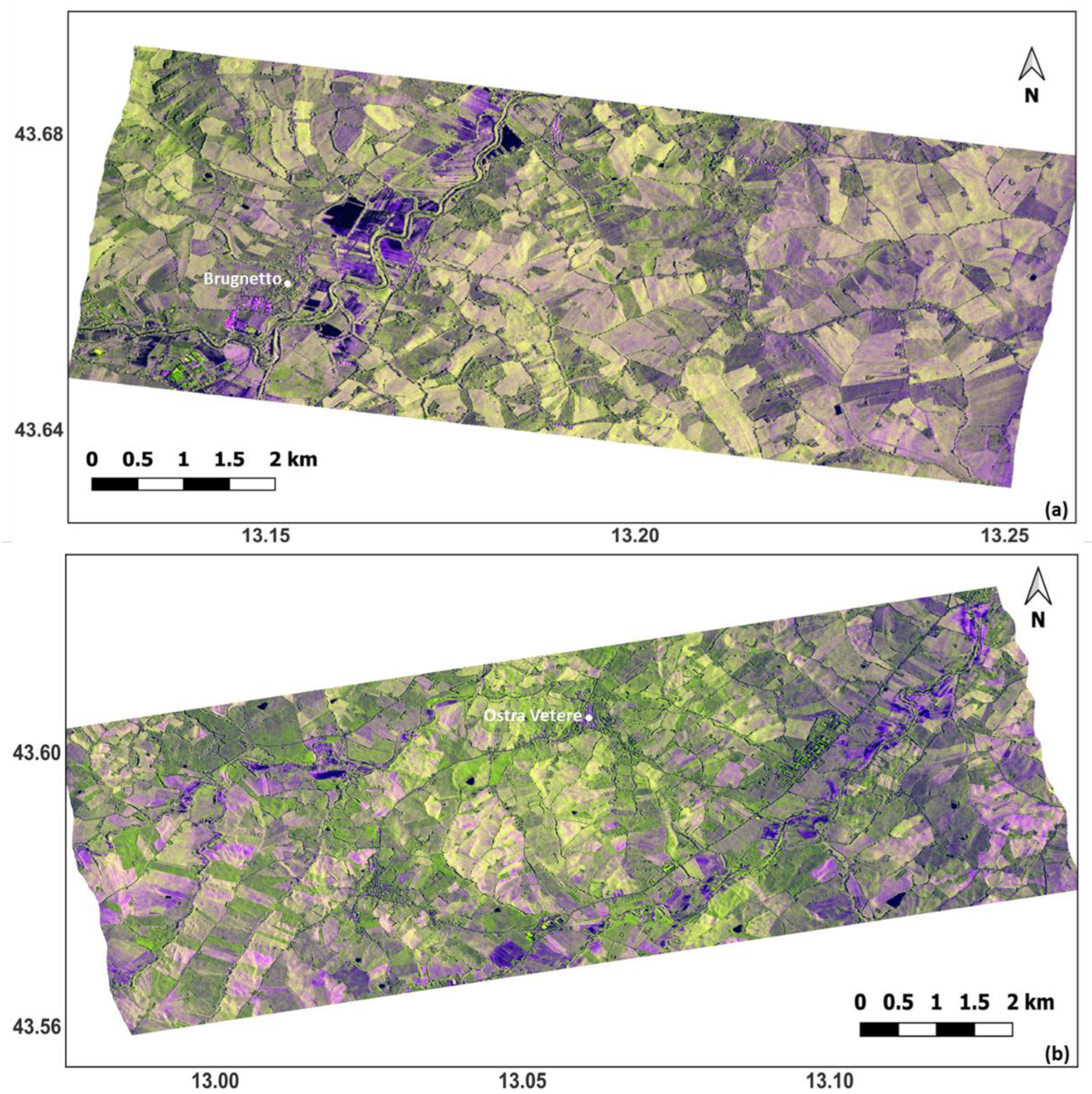
2.2. COSMO-SkyMed Second Generation Dataset and Its Pre-Processing

The CSG is a constellation financed by the Italian Space Agency (ASI) with funds allocated by the Italian Ministry of University and Research, alongside the Italian Ministry of Defense. Similar to the CSK, the CSG is defined as a dual system (civil and military). It consists of two SAR satellites working at the X-band (9.6 GHz) in different imaging modes (Spotlight, Stripmap, PingPong, QuadPol, and ScanSAR) with different resolutions and coverage. More precisely, CSG-1 was launched on 18 December 2019, while CSG-2 was launched on 31 January 2022, and both of them orbit at a mean altitude of 619.6 km (sun-synchronous polar orbit) with a repetition cycle of 16 days.

The only available CSG images of the Marche flood were acquired on 17 September 2022 at 17:00 UTC by CSG-1 (magenta rectangle in Figure 1c) and on 18 September 2022 at 04:40 UTC by CSG-2 (red rectangle in Figure 1c), with incidence angles of 44° and 31°, respectively. The acquisitions were performed in the dual polarization (HH-HV) and spotlight-2C modes. In this configuration, they cover a swath of 5 × 10 km with a resolution of 0.8 × 0.8 m (azimuth × range). The data were calibrated and geocoded by means of the ENVI/SARscape^® software using a 2 m resolution lidar DEM (made available by the Marche region through the Italian Department of Civil Protection) to derive the backscattering coefficient σ⁰.

A common visualization approach for analyzing dual polarized SAR data is the RGB (red–green–blue) channel combination to create a false color composite. The two color composite images shown in Figure 2 were produced by combining σ⁰_HH (red), σ⁰_HV (green), and σ⁰_HH − σ⁰_HV (blue), where the backscattering coefficients are expressed in dB units, that is, σ⁰_dB = 10 × log₁₀(σ⁰) (then, σ⁰_HHdB − σ⁰_HVdB corresponds to σ⁰_HH/σ⁰_HV in linear units). This band combination highlights differences in scattering behavior, thus enabling us to infer information about the surface characteristics. In the following, we refer to dB units and the subscript dB will be omitted for concision.

The geographic zone observed on 17 September is denoted hereafter as the Brugnetto area (Figure 2a), while the geographic zone observed on 18 September is denoted as the Ostra Vetere area (Figure 2b). Brugnetto and Ostra Vetere are two small towns placed in the areas observed by the CSG.

2.3. Ancillary Data

The lack of CSG pre-flood data made it necessary to gather as much information as possible to produce reliable flood maps. Since the areas of interest are mainly rural, it was important to distinguish between bare and vegetated fields. The Normalized Difference Vegetation Index (NDVI) is a simple spectral index that provides this kind of information. A Sentinel-2 (S-2) image acquired on 12 September 2022 was processed to generate an NDVI map. The NDVI map was originally produced at a resolution of 10 m (the resolution of the visible and near infrared S-2 bands) and successively oversampled at 1 m through a cubic convolution. Finally, it was reprojected onto the spatial grid of the CSG images. Although the different spatial resolution between the CSG and the S-2 represents a criticality, the S-2 image was mainly used to compute the mean NDVI value of the objects considered in the data analysis presented in Section 2.5 or identified by the ISODATA clustering described in Section 2.6.2.

The results of the processing of the S-2 image are shown in Figure 3, where the Misa River and the Nevola River are highlighted in dark blue. To precisely identify them in the satellite images, we took advantage of the availability, in vector (shapefile) format, of the hydrological network of the areas affected by the flood.

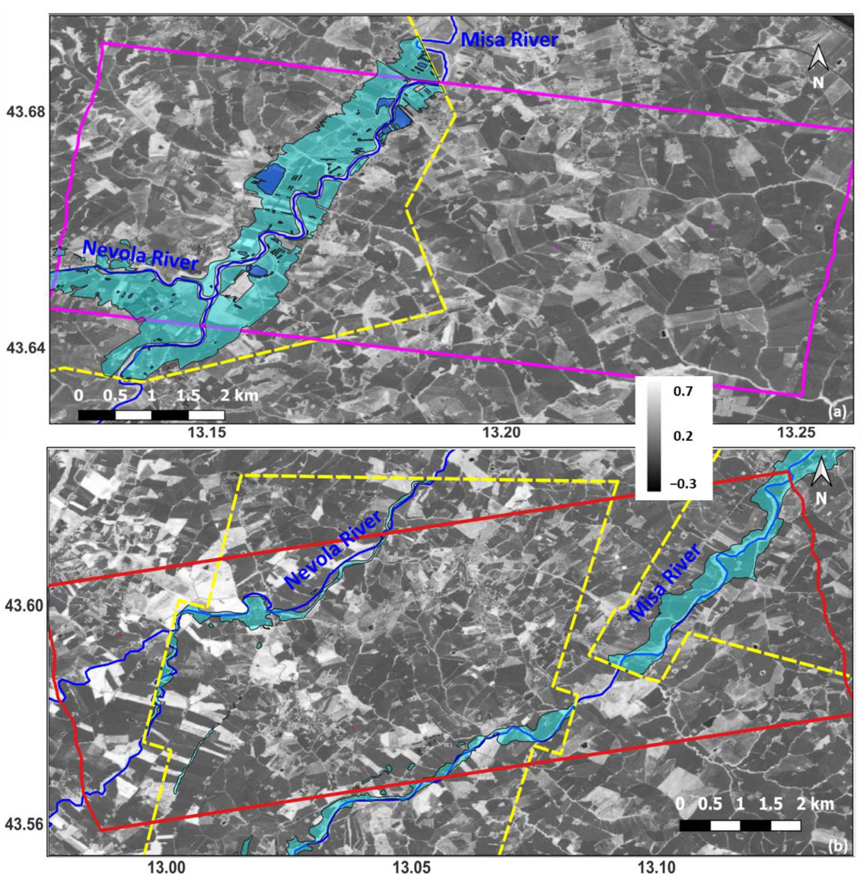
2.4. Reference Data

The flood maps generated by the rapid mapping component of the Copernicus Emergency Management Service (CEMS) were used as reference data. Among the products generated by the CEMS for the Marche flood (available at https://emergency.copernicus.eu/mapping/list-of-components/EMSR634, accessed on 24 February 2023), the maps derived from the very high-resolution acquisitions performed by the WorldView-2 and the Pleaides on 18 September 2022 were chosen. These maps represent grading products in which the flood trace is delineated. They were produced by means of visual interpretation. In general, the flood trace can be visible in optical images even after the event because vegetation or crops could have changed their look since they have been soaked with water, or the terrain could still be very wet and look different on the satellite image with respect to dry terrain. The flood trace basically corresponds to the maximum water extent. In Figure 3, it was superimposed onto the NDVI maps.

For the Brugnetto area (magenta in Figure 3a), the map produced by the CEMS (which makes reference to the Trecastelli town, not imaged by CSG) included some flooded areas inside the flood trace. Conversely, in the Ostra Vetere area (red in Figure 3b), no flooded pixels were present in the CEMS-derived map (which makes reference to the Barbara and Ostra towns) and the flood trace was delineated. The fast water receding that characterized the 2022 Marche flood is the reason why few (or no) flooded areas were present on 17 and 18 September in the areas observed by CSG. Figure 4 shows the water level measured at a station placed in the Brugnetto area (Misa River). The water level had a peak in the evening of 15 September and then decreased rapidly.

2.5. Data Analysis

Some dark blue areas, corresponding to water surfaces where specular scattering is the predominant effect (low σ⁰_HH and very low σ⁰_HV), are clearly visible in Figure 2, especially in the upper panel, which is relative to a CSG acquisition closer in time to the flood peak. Looking at Figure 3, most of the fields were bare (dark in the NDVI maps), but some densely vegetated fields (bright in the NDVI maps) were present too. Some of them were likely affected by the flood being placed near the Misa River and the Nevola River.

The following analysis is focused on the fields shown in Figure 5, which were selected through a visual analysis of the CSG images and the NDVI maps. In particular, Figure 5 was produced to represent the different conditions of the fields inside the areas of interest. The mean values of σ⁰_HH, σ⁰_HV, σ⁰_HH − σ⁰_HV, and NDVI in the fields displayed in Figure 5 are reported in

Table 1. Mean values σ⁰_HH, σ⁰_HV, σ⁰_HH − σ⁰_HV, and NDVI in the fields shown in Figure 5.

Field N°	σ0HH (dB)	σ0HV (dB)	σ0HH − σ0HV (dB)	Avg NDVI
1	−21.0	−25.3	4.2	0.12
2	−21.8	−25.3	3.5	0.45
3	−11.4	−21.6	10.2	0.12
4	−11.7	−19.2	7.5	0.11
5	−5.6	−13.0	7.4	0.07
6	−13.6	−18.1	4.6	0.55
7	−7.9	−15.5	7.6	0.68

.

The blue areas that are visible in the false color composite derived from the CSG images include both bare flooded soils (e.g., Field 1 highlighted by the yellow ellipses in Figure 5a,b, where NDVI is low) and submerged vegetation (e.g., Field 2, orange ellipses in Figure 5a,b, high NDVI).

The microwave signature of the areas appearing as purple-violet in the RGB composite is quite ambiguous. Some of these areas were close to the rivers and the dark areas corresponding to water surfaces (e.g., Field 3, orange ellipses in Figure 5c,d), but fields appearing pale violet were also located far from the areas likely affected by the flood (e.g., Field 4 in Figure 5e,f). These fields were moist (quite high σ⁰_HH, in the order of −11.5 dB in Fields 3-4) and smooth (low σ⁰_HV, in the order of −19/−21 dB in Fields 3-4). They were also bare or scarcely vegetated (mean value of NDVI less than 0.15). Our interpretation is that the very high difference between σ⁰_HH and σ⁰_HV in the fields close to rivers and flooded areas (e.g., 10.2 dB in Field 3) was due to the receding of floodwater that significantly smoothened the soil. Moreover, small ponds inside the humid soil were likely present (dark pixels inside the area that appears purple in Figure 5c); they were detected thanks to the very high resolution of CSG spotlight imagery.

Bare or scarcely vegetated rough and moist fields appear pale green-yellow in the RGB composite (both σ⁰_HH and σ⁰_HV were high, e.g., Field 5 in Figure 5g,h), while most of the vegetated areas appear green because volume scattering was the prevailing effect (low σ⁰_HH − σ⁰_HV, e.g., Field 6 in Figure 5i–l). Not all the vegetated fields appear green in the RGB composite. Figure 5m,n show a vegetated field (average NDVI equal to 0.68), where most of the pixels are yellow in the RGB composite, although violet pixels are present too. This field (Field 7, highlighted by the orange ellipses) was close to the flooded areas and to the Misa River. Moreover, the average value of σ⁰_HH was quite high (−7.9 dB), and the same applies for the average value of σ⁰_HH − σ⁰_HV (7.6 dB, versus 4.6 dB of Field 6). This is likely a case where water was present beneath vegetation and the double-bounce effect involving the smooth water surface and the vertical stems of the plants took place. In addition, the average value of σ⁰_HH was consistent with the backscattering from flooded vegetation simulated in [4] and measured in [14]. Note that a more detectable double-bounce effect is visible in the lower left part of Figure 2a, where bright pink pixels, corresponding to buildings that were oriented orthogonally to the radar look direction, are present. However, flooded built-up areas can be reliably detected based on the increase in the intensity of the double-bounce effect due to floodwater or the decrease in the co-event SAR coherence with respect to the pre-event one [3,4,5,21]. This is possible if two interferometric pairs (pre- and co-event) are available. Since in this study no pre-flood image is available, hereafter, built-up areas will not be considered.

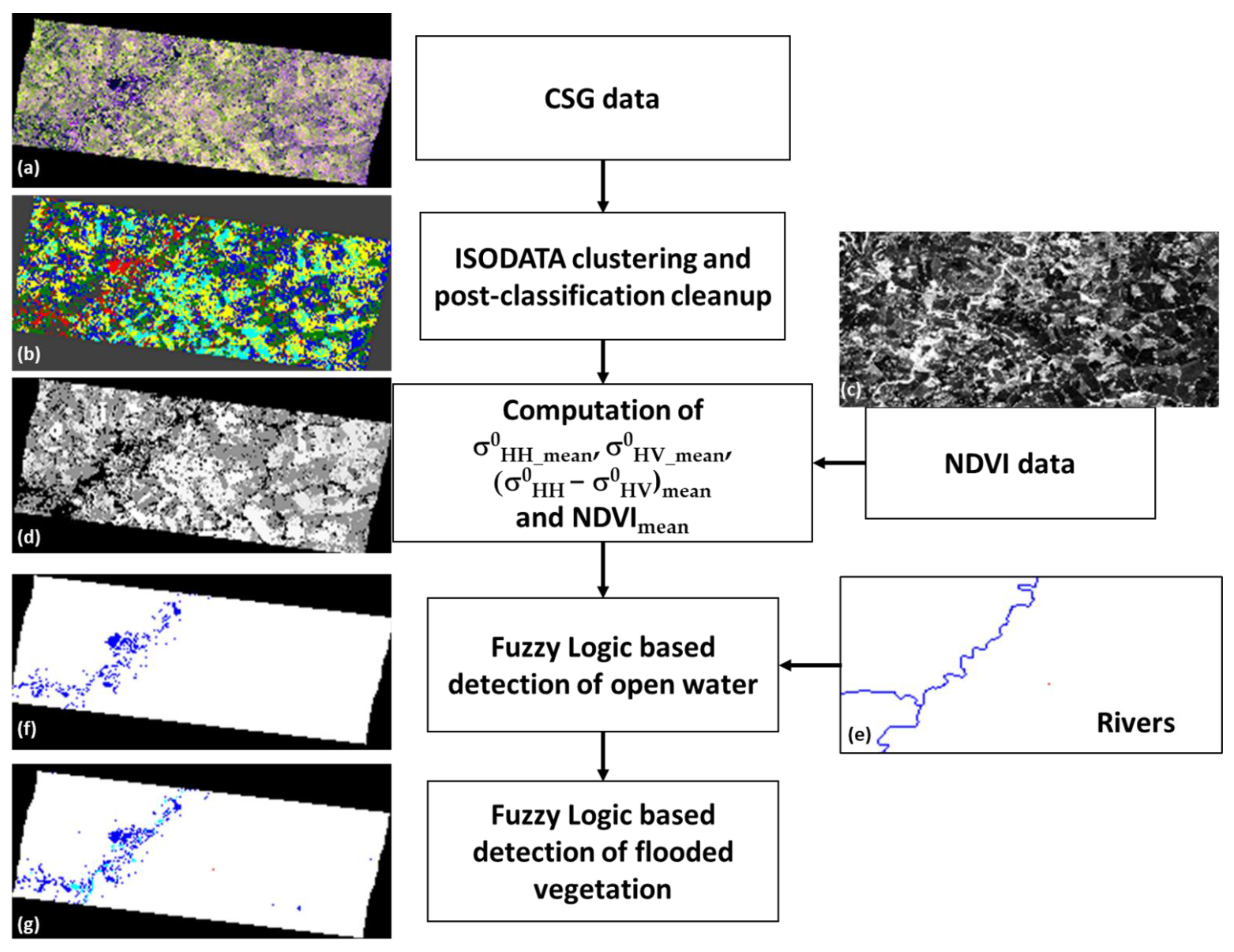
2.6. Flood Mapping Methodology

The flood mapping methodology used to map the Marche flood was based on an adaptation of the AUTOWADE (Automatic Water Areas Detector) algorithm proposed in [10] to high-resolution single SAR images. Not only SAR data but also NDVI ones and data regarding the distance from the rivers were considered to compensate for the lack of pre-flood data. With respect to the AUTOWADE, the methodology is not fully automated but requires an amount of supervision (again, to compensate for the lack of pre-flood data). The workflow of the methodology is shown in Figure 6.

2.6.1. Overview

A preliminary segmentation of the SAR images performed through an ISODATA clustering, applied to co-polarized data (HH, in this case), was the first step of the flood mapping methodology, as in the AUTOWADE. This step, which allowed us to cope with the speckle noise affecting SAR imagery, is even more important when dealing with high-resolution data as CSG ones because the spatial details of the images are considerably smaller than the dimensions of the objects, resulting in large within-class variances [22,23].

The second step was the computation of the mean value of σ⁰_HH, σ⁰_HV, σ⁰_HH − σ⁰_HV, and NDVI (hereafter, denoted as σ⁰_{HH_mean}, σ⁰_{HV_mean}, (σ⁰_HH − σ⁰_HV)_mean and NDVI_mean) in the objects included in the cluster corresponding to the highest values of σ⁰_HH (see Section 2.6.2). Moreover, σ⁰_{HH_mean} was calculated also considering the objects included in the cluster corresponding to the lowest values of σ⁰_HH. Then, a procedure taking advantage of the fuzzy logic and based on σ⁰_{HH_mean} and on the distance from the rivers of the objects’ centroids was applied to detect open water. Note that, in this study, open water includes permanent water and floodwater with no emergent vegetation (i.e., submerged vegetation too). Fuzzy logic was also applied to map flooded vegetation (floodwater with emergent vegetation). For this purpose, σ⁰_{HV_mean}, (σ⁰_HH − σ⁰_HV)_mean, and the distance from open water were considered too.

2.6.2. ISODATA Clustering

The ISODATA is an unsupervised algorithm that separates groups of objects in a scene. Objects within each cluster should be as close to each other as possible and as far from other objects in other clusters as possible [19]. The ISODATA begins with arbitrary cluster means, and then, it clusters the pixels according to the minimum spectral distance technique. It is an iterative procedure in which each iteration recalculates means and reclassifies pixels with respect to the new means. It requires specifying a range for the number of clusters and a maximum number of iterations. The maximum number of interactions was set at 5. While in [10] the maximum number of clusters was set at 10, for this study, it was set at 5 to avoid an over-segmentation of the fields due to the small spatial details of CSG images.

As mentioned above, the ISODATA was applied only to the HH backscattering data because, from the analysis presented in Section 2.5, it can be deduced that HH data are more suitable for open water mapping with respect to HV ones. Low HV values (<−21 dB, see Table 1) were, for instance, found in Field 3, which was not flooded because σ⁰_HH was quite high (>−12 dB).

The result of the application of the ISODATA to the HH data acquired on 17 September 2022 (Brugnetto area) is shown in Figure 6b. Cluster 1 (red in Figure 6b) includes objects whose σ⁰_HH is low, while Cluster 4 and especially Cluster 5 (yellow and cyan, respectively in Figure 6b) include objects whose σ⁰_HH is high. By performing a combined visual analysis of the ISODATA outputs and the CSG images, Cluster 4 and Cluster 5 had to be joined in one cluster (hereafter denoted as Clusters 4-5) to avoid residual over-segmentation of vegetated fields.

To further tackle the problem of the spatial details of the images, which are generally smaller than the dimensions of the typical objects in the scene, a post-classification cleanup process was carried out to avoid the presence of small regions in the ISODATA output. This process consisted of the aggregation of smaller class regions to a larger, adjacent region. A minimum size of the regions of 50 m² was chosen for the aggregation task.

2.6.3. Fuzzy Logic

The availability of single SAR images through the CSG constellation did not allow us to apply any change detection technique to map the flooded areas. Therefore, SAR data were integrated with other kind of data to obtain a good classification accuracy. Different integration methods are available in the literature. Data assimilation methods were designed to integrate remote sensing observations, with estimates from geophysical models [24]. Different methods for combining different sources of information in a probabilistic framework were described in [25]. The use of entropy-based weighting to integrate multiple data sources was proposed in [26]. In [27], data integration was expressed as the problem of combining probability distributions conditioned to each individual datum or data event into a posterior probability for the unknown conditioned jointly to all data. A discussion on data aggregation based on probability from a geostatistical point of view was provided in [28].

The fuzzy logic [20] represents an effective technique to handle ambiguous information sources that are affected by an amount of uncertainty that must be taken into account. It is based on the fuzzy set theory, which is a generalization of the classical set theory. Elements of a fuzzy set have degrees of membership (d_m) to the set, which are defined through membership functions, whose values are real numbers between zero (no membership) and one (maximum membership). Fuzzy logic was chosen because it was widely employed to map flooded areas from SAR data (e.g., [11,29,30]) using very simple membership functions. In particular, the Z and S functions, shown in Figure 7, were often used in flood mapping applications. They are defined as follows [17]:

$$S\left(x\right)=\left\{\begin{array}{cc}0& x\le x_1\hfill \\ 2{\left[(x-x_1)/(x_2-x_1)\right]}^2\hfill & x_1\le x\le (x_1+x_2)/2\hfill \\ 1-2{\left[(x-x_2)/(x_2-x_1)\right]}^2\hfill & (x_1+x_2)/2\le x\le x_2\hfill \\ 1& x>x_2\hfill \end{array}\right.$$

(1)

$$Z\left(x\right)=\left\{\begin{array}{cc}1& x\le x_1\hfill \\ 1-2{\left[(x-x_1)/(x_2-x_1)\right]}^2\hfill & x_1\le x\le (x_1+x_2)/2\hfill \\ 2{\left[(x-x_2)/(x_2-x_1)\right]}^2\hfill & (x_1+x_2)/2\le x\le x_2\hfill \\ 0& x>x_2\hfill \end{array}\right.$$

(2)

where x₁ and x₂ are the fuzzy parameters that, in this study, were determined both in an automated way and through supervision.

2.6.4. Detection of Open Water

The objects belonging to Cluster 1 (i.e., whose HH backscattering was low) were considered to map open water. For these objects, both σ⁰_{HH_mean} and the distance of the centroids from the rivers (dist_R) were computed. Then, the fuzzy set of open water was built by applying the Z function to σ⁰_{HH_mean} and dist_R. Through the Z function, high membership to the set was given to objects presenting low values of σ⁰_{HH_mean} and dist_R (i.e., dark areas close to the rivers in the SAR images).

For Z(σ⁰_{HH_mean}), x₁ and x₂ were determined by using an approach developed in [10]. Firstly, the Roberts filter was applied to the ISODATA outputs, in order to identify the edges of the objects belonging to Cluster 1, which potentially represent water–land edges. To consider actual water–land edges, only objects including pixels with NDVI < 0, likely corresponding to permanent water bodies, were selected. Then, a buffer was created around the edges to include both land and water pixels. Using only the pixels in the buffer, we were able to produce, for each CSG acquisition, a bimodal histogram of the σ⁰_HH values. One mode was relative to the population of water pixels, and the other mode was relative to the population of land pixels. The bimodal histogram was successively fitted by two Gaussian functions through a non-linear fit [8] (thus assuming a Gaussian mixture model). By denoting as th_Otsu the threshold value computed by applying the Otsu thresholding method [31] to the bimodal histogram, and by m and s the mean value and standard deviation of the Gaussian distribution fitting the histogram of the water pixels included in the buffer, x₁ and x₂ were computed as follows [10]:

$$x_1=0.5\cdot ({th}_{Otsu}+m)$$

(3)

$$x_2=(m+2s)$$

(4)

To determine the parameter x₂ of Z(dist_R), a visual analysis of the CSG images was carried out. The objective was to find the value of dist_R beyond which no flooded areas were present in the scenes. For the Brugnetto area, x₂ was set at 1 km, while for the Ostra Vetere area, x₂ was set at 400 m. In both cases, x₁ was set at 0. The degree of membership to the set of open water was computed by averaging the degrees obtained by applying the Z function to σ⁰_{HH_mean} and dist_R. The objects presenting an average degree greater than 0.5 were assigned to the class of open water.

2.6.5. Detection of Flooded Vegetation

To map flooded vegetation, the objects included in Clusters 4-5 (i.e., whose HH backscattering was high) having NDVI_mean ≥ 0.25 were considered. Objects with NDVI_mean < 0.25 were assumed as bare or scarcely vegetated and discarded for this analysis. For the selected objects, σ⁰_{HH_mean}, σ⁰_{HV_mean}, (σ⁰_HH − σ⁰_HV)_mean, and dist_R were computed, together with another distance, that is, the minimum distance of an object from open water (dist_W). The rationale was to consider, as possibly flooded, only vegetated fields adjacent to open water.

To build the fuzzy set of flooded vegetation, the S function was applied to σ⁰_{HH_mean} and (σ⁰_HH − σ⁰_HV)_mean. In this way, a high membership to the fuzzy set was given to the objects where an intense double-bounce effect likely took place, i.e., where both σ⁰_{HH_mean} and (σ⁰_HH − σ⁰_HV)_mean were high. For S(σ⁰_{HH_mean}), x₁ and x₂ were determined based on the results reported in Table 1 concerning Field 6 (non-flooded vegetation) and Field 7 (flooded vegetation), which were included in the Brugnetto area. For the CSG observation of the latter area, x₁ was set at −10 dB, a value considerably larger than σ⁰_{HH_mean} of Field 6; x₂ was set at −6 dB (larger than σ⁰_{HH_mean} of Field 7). For the image of the Ostra Vetere area (18 September), the values of x₁ and x₂ were modified to account for the different incidence angle (θ) by assuming that the variation in σ⁰ with θ can be approximated by cos²(θ) [32]. As for (σ⁰_HH − σ⁰_HV)_mean, x₁ was set at 6.5 dB (larger than (σ⁰_HH − σ⁰_HV)_mean of Field 6) and x₂ at 8.5 dB (larger than (σ⁰_HH − σ⁰_HV)_mean of Field 7).

The Z function was applied to give high membership to the fuzzy set of flooded vegetation to objects presenting low values of σ⁰_{HV_mean} (considering that the double-bounce effect generally does not give rise to depolarization) and of dist_R and dist_W. Regarding Z(σ⁰_{HV_mean}), the values of x₁ and x₂ were again determined based on the results of Table 1. For the image of the Brugnetto area, x₁ was set at −18 dB and x₂ was set at −14 dB. For the image of the Ostra Vetere area, the values of x₁ and x₂ were again modified based on the cos²(θ) assumption. For Z(dist_R), we maintained the same values used for open water, while for Z(dist_W), x₁ was set at 0 and x₂ was set at 20 m for both the CSG acquisitions.

Even in this case, the different degrees of membership computed as described above were averaged and the objects presenting an average degree greater than 0.5 were assigned to the class of flooded vegetation.

2.7. Validation

To verify the reliability of the methodology described in Section 2.6, the reference data introduced in Section 2.4 were exploited. As in [10], a confusion matrix was derived to compute the number of pixels assigned to a particular class relative to the actual class, as indicated by the reference data. In this case, the reference data discriminate only one class (flooded areas) from the background. This class represents a positive case, while the background represents a negative case. Then, the terms true positive (TP), false positive (FP), true negative (TN), and false negative (FN) are used.

The confusion matrix was calculated considering the spatial domain defined by the “area of interest” shapefile included in the CEMS products. In [10], the F1-score and the errors of commission (ε_comm) and omission (ε_om) were used as main accuracy metrics. The errors are defined as follows:

$${\epsilon }_{comm}=\frac{FP}{TP+FP}$$

(5)

$${\epsilon }_{om}=\frac{FN}{TP+FN}$$

(6)

The F1-score is defined as follows:

$$F1-score=\frac{2\times Precision\times Recall}{Precision+Recall}$$

(7)

where

$$Precision=1-{\epsilon }_{comm}$$

(8)

$$Recall=1-{\epsilon }_{om}$$

(9)

For the Marche flood case study, we had to consider that the Brugnetto area was observed by CSG on 17 September 2022 and by Pleiades (used to generate the CEMS product) the day after. Since, reportedly, the water receded between 17 and 18 September, the commission error was evaluated considering the flood objects outside the flood trace delineated by the CEMS using the Pleiades image. As for the Ostra Vetere area, no flooded pixels were present in the CEMS-derived map. Then, only ε_comm was evaluated, again considering the flood objects outside the flood trace delineated by the CEMS, because otherwise, a value of 100% for ε_comm would have been obtained.

3. Results

The maps of flooded areas generated by applying the methodology described in Section 2.6 are shown in Figure 8.

In Figure 8a (17 September), a greater number of flooded pixels is present with respect to Figure 8b (18 September), mainly because of the water receding. Note that, even on 18 September, when all the images used to generate the CEMS products were acquired, more water was present in the Brugnetto area with respect to the Ostra Vetere area (see Figure 3).

As for the accuracy metrics, the following values were obtained for the Brugnetto area: F1-score = 90.5%, ε_comm = 12.3%, ε_om = 6.3%. For the Ostra Vetere area, only ε_comm was evaluated (see Section 2.7), obtaining a value equal to 11.7%. Figure 9 shows the details of the false positives (related to the commission error) and the false negatives (related to the omission error). In agreement with the considerations made at the end of Section 2.7, only false positives are present in Figure 9b (Ostra Vetere area).

4. Discussion

This paper presented an analysis of the CSG data used to monitor a flood that occurred in a central region of Italy (Marche) in 2022. They were acquired in the spotlight and dual polarization (HH-HV) modes, with a spatial resolution finer than 1 m (0.8 × 0.8 m²). Although studies on flood mapping using COSMO-SkyMed are available in the literature [4,14,15,17,33], to the best of authors’ knowledge this is the first paper where data provided by the Second Generation of the COSMO-SkyMed constellation were exploited.

The importance of this study is related to the on-demand capabilities of the CSG (further improved with respect to the capabilities of the CSK), which makes it possible to reduce the number of missed floods. However, the capability of the CSG to promptly respond to users’ request implies that pre-flood images acquired with the same observation geometry of the flood images are not generally available. Then, to fully exploit the technological advantages offered by the CSG, a detailed analysis of the mono-temporal radar signatures of the flooded areas was carried out. Conversely, in previous papers regarding the use of CSK images for flood mapping, multi-temporal data were processed [4,14,33].

The use of single SAR images provided by a new constellation of satellites is required to perform a supervised analysis. For this purpose, we also used ancillary data, such as an NDVI map derived from a S-2 acquisition, and information about the distance of the objects identified in the SAR images with respect to the rivers (dist_R) present in the scenes. While the joint analysis of the CSG images and the ISODATA outputs that led us to merge Cluster 4 and Cluster 5 (Section 2.6.2) did not require much effort, the determination of the values of the fuzzy parameters (Section 2.6.4 and Section 2.6.5) required a detailed analysis of the available data. This analysis included the selection of fields used as a reference to represent the different targets in the scenes and the computation of the mean backscattering values in these fields. The need to perform this kind of analysis can be considered as a limitation with respect to fully automated algorithms developed for other sensors like Sentinel-1 (e.g., [8,9,10,11,34]).

The data regarding vegetation turned out to be fundamental to distinguishing rough bare soils from flooded vegetation. Their radar signatures were quite similar, although flooded vegetation generally presented smaller values of σ⁰_HV because the prevailing effect produced by this target on the radar backscattering is the double bounce that does not produce depolarization. Mapping flooded vegetation is still a challenging task even when using time series of data, as for instance, in [35,36]. In our study, this task was further complicated by the use of single SAR images. To increase the reliability of the detection of flooded vegetation, we exploited not only the information provided by dist_R but also the information about the distance from open water (dist_W), limiting the search for flooded vegetation to areas very close or even adjacent to open water.

The use of dist_R in open water detection allowed us to mitigate the problem of the misclassification of targets appearing dark in SAR images (e.g., roads). They can be detected (and masked) by applying change detection techniques; otherwise, they can be generally confused with flooded areas. Note that supervision was necessary to mask roads and built up-areas included in urban settlements.

As suggested in previous papers [4,14], a fundamental step of flood mapping from high-resolution SAR data was image segmentation, which allowed us to account for the relation between the spatial resolution and the dimensions of target objects. As underlined in [37], for images having sub-metric geometric resolution (such as CSG ones), an approach to properly consider this relation consists of merging pixels into objects (i.e., image segmentation). In [4,14], quite sophisticated approaches for image segmentation were applied, while here, to account for the timeliness requirement that is generally important for flood mapping applications, a quite simple ISODATA clustering was adopted.

The fuzzy logic allowed us to integrate different sources of data in order to increase the flood mapping accuracy in a quite simple way, although more sophisticated data aggregation methods are available in the literature. In agreement with the previous discussion, the fuzzy membership functions were applied to the objects identified by the ISODATA and not to the image pixels.

Good results were obtained when comparing the flood maps generated by applying the methodology proposed in this paper with the maps produced by the Copernicus Emergency Service (rapid mapping component) for the 2022 Marche flood using optical data. For the Brugnetto area, a very low omission error was obtained, while the commission error was higher. Most of the false positives were due to roads close to the rivers (orange pixels in the middle part of Figure 9) for which dist_R was not useful to avoid misclassification. In addition, in the CEMS-derived maps, rivers were excluded from the classification, while they were included in our maps (orange pixels in the lower left part of Figure 9). These differences could be expected considering that our maps were generated without performing a change detection task. For the Ostra Vetere area, only the commission error was computed. In this case, false positives were mostly produced by areas placed outside the boundaries of the flood trace that appeared dark in the CSG image.

It must be pointed out that, to compute the accuracy metrics, we had to consider the time difference between the CSG and the Pleiades observations of the Brugnetto area. Moreover, no flooded areas were detected by the CEMS in the Ostra Vetere area. Then, the commission error had to be evaluated based on the flood objects placed outside the flood trace delineated in the CEMS products. Further studies are therefore needed to evaluate the reliability of the flood mapping procedure proposed in this paper.

5. Conclusions

The results of an experience gained by analyzing and processing the COSMO-SkyMed Second Generation X-band radar images collected during a flood event that occurred in the Marche region (central Italy) in September 2022 were presented. The data were acquired at sub-metric spatial resolution (spotlight mode) and in the dual polarization (HH-HV) mode. It was shown that, to produce a detailed and thematically accurate flood map, it was necessary to perform a detailed analysis of the different radar signatures of the various targets present in the scene, such as rough bare fields, smooth moist fields, densely vegetated fields, water surfaces, and flooded vegetation. The analysis was supported by the use of NDVI data derived from a Sentinel-2 image acquired a few days before the flood.

Based on the outcomes of the aforementioned analysis, a flood mapping procedure was designed. It was based on a preliminary image segmentation that allowed us to merge pixels into objects. In this way, we accounted for the spatial details of the CSG images, which were considerably smaller than the dimensions of the objects in the scene. The fuzzy logic was then applied to integrate the SAR data with the ancillary data. This integration allowed us to (at least partially) compensate for the lack of pre-flood images.

Good results were obtained by comparing the flood maps produced using CSG data with those generated by the Copernicus Emergency Service. However, other investigations are necessary to consolidate the flood mapping procedure proposed in this study and to reduce the amount of supervision requested by the procedure.

References

- Shen, X.; Wang, D.; Mao, K.; Anagnostou, E.; Hong, Y. Inundation extent mapping by synthetic aperture radar: A review. Remote Sens. 2019, 11, 879. [Google Scholar] [CrossRef] [Green Version]
- Pierdicca, N.; Pulvirenti, L.; Chini, M.; Guerriero, L.; Candela, L. Observing floods from space: Experience gained from COSMO-SkyMed observations. Acta Astronaut. 2013, 84, 122–133. [Google Scholar]
- Chini, M.; Pelich, R.; Pulvirenti, L.; Pierdicca, N.; Hostache, R.; Matgen, P. Sentinel-1 InSAR Coherence to Detect Floodwater in Urban Areas: Houston and Hurricane Harvey as A Test Case. Remote Sens. 2019, 11, 107. [Google Scholar] [CrossRef] [Green Version]
- Pulvirenti, L.; Chini, M.; Pierdicca, N.; Boni, G. Use of SAR data for detecting floodwater in urban and agricultural areas: The role of the interferometric coherence. IEEE Trans. Geosci. Remote Sens. 2016, 54, 1532–1544. [Google Scholar] [CrossRef]
- Pelich, R.; Chini, M.; Hostache, R.; Matgen, P.; Pulvirenti, L.; Pierdicca, N. Mapping Floods in Urban Areas from Dual-Polarization InSAR Coherence Data. IEEE Geosci. Remote Sens. Lett. 2022, 19, 4018405. [Google Scholar] [CrossRef]
- Giustarini, L.; Hostache, R.; Matgen, P.; Schumann, G.-P.; Bates, P.D.; Mason, D.C. A change detection approach to flood mapping in urban areas using TerraSAR-X. Geosci. Remote Sens. IEEE Trans. 2013, 51, 2417–2430. [Google Scholar] [CrossRef] [Green Version]
- Mason, D.C.; Dance, S.L.; Cloke, H.L. Floodwater detection in urban areas using Sentinel-1 and WorldDEM data. J. Appl. Remote Sens. 2021, 15, 032003. [Google Scholar] [CrossRef]
- Chini, M.; Hostache, R.; Giustarini, L.; Matgen, P. A hierarchical split-based approach for parametric thresholding of SAR images: Flood inundation as a test case. IEEE Trans. Geosci. Remote Sens. 2017, 55, 6975–6988. [Google Scholar]
- Landuyt, L.; Van Coillie, F.M.B.; Vogels, B.; Dewelde, J.; Verhoest, N.E.C. Towards operational flood monitoring in flanders using sentinel-1. IEEE J. Sel. Top. Appl. Earth Obs. Remote Sens. 2021, 14, 11004–11018. [Google Scholar] [CrossRef]
- Pulvirenti, L.; Squicciarino, G.; Fiori, E.; Ferraris, L.; Puca, S. A Tool for Pre-Operational Daily Mapping of Floods and Permanent Water Using Sentinel-1 Data. Remote Sens. 2021, 13, 1342. [Google Scholar]
- Martinis, S.; Kersten, J.; Twele, A. A fully automated TerraSAR-X based flood service. ISPRS J. Photogramm. Remote Sens. 2015, 104, 203–212. [Google Scholar]
- Salamon, P.; McCormick, N.; Reimer, C.; Clarke, T.; Bauer-Marschallinger, B.; Wagner, W.; Martinis, S.; Chow, C.; Böhnke, C.; Matgen, P.; et al. The New, Systematic Global Flood Monitoring Product Of The Copernicus Emergency Management Service. In Proceedings of the International Geoscience and Remote Sensing Symposium (IGARSS), Brussels, Belgium, 11–16 July 2021; pp. 1053–1056. [Google Scholar]
- Pulvirenti, L.; Pierdicca, N.; Chini, M.; Guerriero, L. An algorithm for operational flood mapping from Synthetic Aperture Radar (SAR) data using fuzzy logic. Nat. Hazards Earth Syst. Sci. 2011, 11, 529–540. [Google Scholar] [CrossRef] [Green Version]
- Pulvirenti, L.; Pierdicca, N.; Chini, M.; Guerriero, L. Monitoring flood evolution in vegetated areas using cosmo-skymed data: The tuscany 2009 case study. IEEE J. Sel. Top. Appl. Earth Obs. Remote Sens. 2013, 6, 1807–1816. [Google Scholar] [CrossRef]
- Chini, M.; Pulvirenti, L.; Pierdicca, N. Analysis and interpretation of the COSMO-SkyMed observations of the 2011 Japan tsunami. IEEE Geosci. Remote Sens. Lett. 2012, 9, 467–471. [Google Scholar] [CrossRef]
- Boni, G.; Ferraris, L.; Pulvirenti, L.; Squicciarino, G.; Pierdicca, N.; Candela, L.; Pisani, A.R.; Zoffoli, S.; Onori, R.; Proietti, C.; et al. A Prototype System for Flood Monitoring Based on Flood Forecast Combined with COSMO-SkyMed and Sentinel-1 Data. IEEE J. Sel. Top. Appl. Earth Obs. Remote Sens. 2016, 9, 2794–2805. [Google Scholar] [CrossRef]
- Pulvirenti, L.; Marzano, F.S.; Pierdicca, N.; Mori, S.; Chini, M. Discrimination of water surfaces, heavy rainfall, and wet snow using COSMO-SkyMed observations of severe weather events. IEEE Trans. Geosci. Remote Sens. 2014, 52, 858–869. [Google Scholar] [CrossRef]
- ASI. COSMO-SkyMed Seconda Generazione: System and Products Description. 2021. Available online: https://earth.esa.int/eogateway/documents/20142/37627/COSMO-SkyMed-Second-Generation-Mission-Products-Description.pdf (accessed on 1 February 2023).
- Richards, J.A.; Jia, X. Remote Sensing Digital Image Analysis: An Introduction; Springer: Cham, Switzerland, 2006; ISBN 3540251286. [Google Scholar]
- Zadeh, L.A. Fuzzy sets. Inf. Control 1965, 8, 338–353. [Google Scholar] [CrossRef] [Green Version]
- Pulvirenti, L.; Chini, M.; Pierdicca, N. InSAR Multitemporal Data over Persistent Scatterers to Detect Floodwater in Urban Areas: A Case Study in Beletweyne, Somalia. Remote Sens. 2021, 13, 37. [Google Scholar] [CrossRef]
- Blaschke, T.; Hay, G.J.; Kelly, M.; Lang, S.; Hofmann, P.; Addink, E.; Queiroz Feitosa, R.; van der Meer, F.; van der Werff, H.; van Coillie, F.; et al. Geographic Object-Based Image Analysis—Towards a new paradigm. ISPRS J. Photogramm. Remote Sens. 2014, 87, 180–191. [Google Scholar]
- Pulvirenti, L.; Chini, M.; Pierdicca, N.; Guerriero, L.; Ferrazzoli, P. Flood monitoring using multi-temporal COSMO-skymed data: Image segmentation and signature interpretation. Remote Sens. Environ. 2011, 115, 990–1002. [Google Scholar]
- Reichle, R.H. Data assimilation methods in the Earth sciences. Adv. Water Resour. 2008, 31, 1411–1418. [Google Scholar]
- Allard, D.; Comunian, A.; Renard, P.; Comunian, A.; Renard, P. Probability Aggregation Methods in Geoscience. Math. Geosci. 2012, 44, 545–581. [Google Scholar]
- Hou, W.; Cui, C.; Yang, L.; Yang, Q.; Clarke, K. Entropy-Based Weighting in One-Dimensional Multiple Errors Analysis of Geological Contacts to Model Geological Structure. Math. Geosci. 2019, 51, 29–51. [Google Scholar] [CrossRef]
- Polyakova, E.I.; Journel, A.G.; Polyakova, E.I.; Journel, A.G.; Journel, A.G. The Nu Expression for Probabilistic Data Integration. Math. Geol. 2007, 39, 715–733. [Google Scholar] [CrossRef]
- Mariethoz, G.; Renard, P.; Froidevaux, R. Integrating collocated auxiliary parameters in geostatistical simulations using joint probability distributions and probability aggregation. Water Resour. Res. 2009, 45, 4–7. [Google Scholar]
- Martinis, S.; Twele, A. A hierarchical spatio-temporal Markov model for improved flood mapping using multi-temporal X-band SAR data. Remote Sens. 2010, 2, 2240–2258. [Google Scholar] [CrossRef] [Green Version]
- Pierdicca, N.; Chini, M.; Pulvirenti, L.; Macina, F. Integrating physical and topographic information into a fuzzy scheme to map flooded area by SAR. Sensors 2008, 8, 4151–4164. [Google Scholar] [CrossRef] [Green Version]
- Otsu, N. A Threshold Selection Method from Gray Level Histograms. IEEE Trans. Syst. Man. Cybern. 1979, 9, 62–66. [Google Scholar] [CrossRef] [Green Version]
- Ulaby, F.T.; Dobson, M.C. Handbook of Radar Scattering Statistics for Terrain; Artech House: Norwood, MA, USA, 1989; Volume 1, ISBN 0890063362. [Google Scholar]
- Pierdicca, N.; Pulvirenti, L.; Boni, G.; Squicciarino, G.; Chini, M. Mapping Flooded Vegetation Using COSMO-SkyMed: Comparison with Polarimetric and Optical Data Over Rice Fields. IEEE J. Sel. Top. Appl. Earth Obs. Remote Sens. 2017, 10, 2650–2662. [Google Scholar]
- Bauer-Marschallinger, B.; Cao, S.; Tupas, M.E.; Roth, F.; Navacchi, C.; Melzer, T.; Freeman, V.; Wagner, W. Satellite-Based Flood Mapping through Bayesian Inference from a Sentinel-1 SAR Datacube. Remote Sens. 2022, 14, 3673. [Google Scholar]
- Tsyganskaya, V.; Martinis, S.; Marzahn, P. Flood monitoring in vegetated areas using multitemporal Sentinel-1 data: Impact of time series features. Water 2019, 11, 1938. [Google Scholar] [CrossRef] [Green Version]
- Refice, A.; Zingaro, M.; D’addabbo, A.; Chini, M. Integrating C-and L-band SAR imagery for detailed flood monitoring of remote vegetated areas. Water 2020, 12, 2745. [Google Scholar] [CrossRef]
- Blaschke, T. Object based image analysis for remote sensing. ISPRS J. Photogramm. Remote Sens. 2010, 65, 2–16. [Google Scholar] [CrossRef] [Green Version]