Abstract
Flow motion with complex patterns, such as vortex, stagnant flow, and seepage, put forward higher spatial resolution requirements for particle image velocimetry (PIV). With the development of deep learning technology in optical flow estimation, many attempts have been made to introduce deep learning-based optical flow (DLOF) into PIV. Compared with the traditional optical flow method, the DLOF method has the advantages of higher precision, faster calculation speed, and avoiding manual parameter adjustment. However, DLOF research is generally developed based on the basic characteristics of rigid body motion, and its key loss function part still generally uses the L1 (mean absolute error, MAE, L1) or L2 (mean square error, MSE, L2) loss functions, which lack consideration of fluid motion characteristics. Therefore, the current DLOF research has the problems of large angular error and serious curl-divergence loss in fluid motion estimation scenarios with smaller spatial scales than rigid bodies. Based on the prior knowledge of the traditional fluid motion characteristics, this study proposes a fluid loss function for describing the fluid motion characteristics, and combines this loss function with Flownet2. The compound loss (CL) function is combined with the displacement error, angular error, and div-curl smooth loss. The method combined with the loss function in this paper is called FlowNet2-CL-PIV. In order to verify that the compound loss function proposed in this study has a positive impact on the model training results, this paper uses the cosine similarity measure to demonstrate its effectiveness. In addition, the parameter selection of the compound loss function is analyzed and compared, and it is verified that the best training effect can be achieved by adjusting the parameter so that the order of magnitude of each part of the compound loss function is consistent. In order to test the calculation effect of the Flownet2-CL-PIV method proposed in this study, synthetic particle images are used for model training and performance analysis. Simulation results in various flow fields show that the root mean square error (RMSE) and average angular error (AAE) of Flownet2-CL-PIV reach 0.182 pixels and 1.7°, which are 10% and 54% higher than the original model, respectively.
1. Introduction
Particle image velocimetry technology is a modern flow measurement technology that makes full use of modern material technology, laser technology, digital imaging technology, computer technology, and image analysis technology. It can non-invasively measure the two-dimensional or three-dimensional transient flow field in the plane [1], which provides the possibility for more refined flow observation. With the continuous improvement of the requirements for the accuracy of fluid flow state estimation, the complex flow phenomenon existing in the fluid has become the focus and difficulty of research. Complex flow phenomena generally refer to flow phenomena with characteristics such as transient, pulsating, unsteady, and multi-scale changes, which widely exist in nature and in the fields of industrial production, aerospace, and machinery manufacturing [2,3,4].
The observation of complex flow phenomena provides a demand for observations with higher spatial resolution and higher temporal resolution. In the nearly forty years of particle image velocimetry, the hardware foundation and software methods of PIV measurement technology have made great progress. From the traditional cross-correlation algorithm [5] to the WIDIM [6] algorithm based on window iterative deformation, its measurement accuracy, flow field resolution, and calculation efficiency have all been significantly improved. However, even the WIDIM algorithm, which can almost achieve a single-pixel spatial resolution, is limited by the size of the cross-correlation window and the size of the inquisition area, and it is difficult to take into account both small-scale flow field motion and large-scale flow field observation.
In order to obtain flow fields with higher spatial resolution, there have been many attempts to introduce optical flow estimation methods into PIV measurements. Optical flow estimation is one of the traditional methods in the field of motion estimation. In 1981, after Horn and Schunck first proposed the basic conservation assumption and calculation model of optical flow [7], the research on optical flow calculation and related technologies received extensive attention. After that, a large number of improved algorithms for optical flow estimation were proposed. These methods and studies have greatly improved the accuracy, calculation speed, and robustness of optical flow estimation, making it gradually applicable to practical scenarios. The classic optical flow model is mainly suitable for estimating rigid motion in various natural scenes. However, the brightness constraint equation it relies on is not derived from physical principles, lacks physical explanation, and struggles to capture fluid motion with complex motion patterns. Therefore, in order to enable the optical flow estimation method to be used to estimate fluid motion, Corpetti, T., Liu, T.S., et al. [8,9] combined the fluid motion characteristics, such as the continuity equation of incompressible fluids, to make adaptive improvements to the constraints of optical flow estimation data items, regular items, etc., which gradually led to a suitable physical interpretation of the fluid application of the optical flow estimation method. On this basis, Tauro, F., Khalid, M. et al. [10,11] carried out the research on applying the method of optical flow estimation to the field of PIV.
In recent years, the rise of deep learning technology has led to the emergence of many excellent deep learning optical flow (DLOF) estimation methods. These methods mainly include Liteflownet [12], Flownet [13], PWCnet [14], RAFT [15], and so on. Among them, Flownet first realized the end-to-end dense optical flow estimation through the design of the correlation layer, and designed two models, FlownetS and FlownetC, according to the different feature extraction methods. Since then, the network model Flownet2 [16], obtained by stacking the two structures of Flownet, has improved the accuracy of optical flow estimation to the best level of traditional methods through the application of feature warp technology, network stack, and other technologies.
Since the rise of deep learning technology, attempts to apply the DLOF methods to PIV have gradually emerged. Li Yong first built a regression convolutional neural network for PIV flow field calculation [17]. Although this model realized the end-to-end flow field estimation, its flow field resolution could only reach 1/64, and the calculation efficiency was lower than that of the WIDIM method. The PIV measurement based on deep matching [18] starts from the point of view of feature matching. However, the way of matching the feature corners in the two frames of images can only obtain a sparse flow field due to the sparsity of the feature corners. Cai S also applied the optical flow method to the PIV measurement task by improving the two network structures of Liteflownet and Flownet [19,20] and, for the first time, obtained a flow field with the same resolution as the original image, and achieved a relatively good result in the PIV optical flow estimation task.
The loss function is a crucial part of the deep learning method. It regulates the error between samples and predictions. Studies have shown that the loss function is closely related to the generalization ability and training efficiency of the neural network [21]. The practical significance of the loss function is usually the gap between the ground truth and the prediction result. Compound loss functions can be thought of as simultaneous optimizations for multiple tasks or objectives [22,23]. By combining and optimizing multiple loss functions, the gap between the real value and the predicted value can be narrowed from multiple angles. The L2 loss function used to express the Euclidean space distance between two vectors is usually used in regression analysis such as optical flow estimation.
Since Corpetti, T. et al. [8] improved the data constraint term of traditional optical flow estimation based on the motion characteristics of incompressible fluids, introducing the prior condition of fluid motion into the optical flow method is the key direction of the fluid field application of optical flow calculation. According to the similarity between the loss function and the energy minimization function of traditional optical flow estimation, coupling the prior condition of the fluid motion characteristics with the loss function of the deep learning method improves the physical interpretability of the DLOF method in the field of PIV. Chang-Dong Yu et al. [24] considered the problem of illumination drift in image sequences, and optimized the loss function of Liteflownet for the PIV data set based on the brightness gradient smoothness and first-order curl-divergence smoothing items, and also used the dice loss function improvements to U-net [25] to show good results. These attempts validate that loss functions play a crucial role when applying DLOF methods to the field of fluid motion estimation. Based on the same idea, this study proposes a compound loss function combining RMSE, AAE, and div-curl loss to perform multi-angle targeted optimization of the local and global characteristics of fluid motion.
The work of this study is mainly carried out in the following three parts: In Section 2, the basic structure of the Flownet2 model is introduced first, followed by the improvements made to the model in this study: based on the prior knowledge of fluid motion characteristics, a compound loss function of Euclidean distance error, angular error, and div-curl smooth loss is set. Finally, the generation of simulated particle image data sets through numerical simulation is also introduced in this section, and covers flow field models with various complex motion modes, such as the linear flow field, Hammel-Ossen flow field, Rankine vortex flow field, etc. In Section 3, the index of performance measurement set from the perspectives of RMSE, AAE, and curl-divergence loss is introduced firstly, and secondly, the feasibility and effectiveness of the method in this paper are verified via the cosine similarity of each part of the compound loss function and the sensitivity of the composite parameters. Then, the calculation effect of the compound loss function combination set by the method in this study is compared on the experimental data set, and finally, the method in this study and the Flownet2 model are compared and evaluated using the traditional L2 loss function from the perspective of the calculation effect of different flow fields. Section 4 summarizes and evaluates the method of this study.
2. Approach and Materials
2.1. Flownet2 Network Structure
Since the convolutional neural network technology was developed by Hinton, it has been widely used in various studies. The technology itself is constantly updated and developed. Starting from the most basic convolution, pooling, and fully connected layers, the deep convolutional neural networks built layer by layer have achieved excellent results in various computing tasks. Neural networks have also become an increasingly practical computing tool.
FlownetS and FlownetC are among the first convolutional neural networks used for optical flow estimation. Deep learning methods actually give an excellent feature extraction scheme. However, optical flow estimation still needs to reconstruct the flow field. Therefore, although the above two networks are different in feature extraction, the same deconvolution network is used in the subsequent layer-by-layer optical flow estimation.
FlownetS is designed on the basis of a simple method of directly stacking two 3-channel images into a 6-channel one. FlownetC proposes the use of a feature extraction network with shared weights to extract the features of the two frames of images separately, and then the use of the correlation layer to fuse them. Although the correlation layer neural network designed by FlownetC based on the traditional cross-correlation method greatly improves the parameter complexity, it also improves the accuracy of optical flow estimation in terms of results, and it provides the basis for the Flownet2 stacking network.
On the basis of FlownetC and FlownetS, network stacking and image warping are used to deepen the network to improve computing power, sub-network modules are designed for large and small displacements, respectively, and a new network model, Flownet2, is formed in combination. The ability of optical flow estimation has reached the best level of traditional methods, and the calculation speed can reach 8 fps. The Flownet2 network model is shown in Figure 1. By stacking the network, combining image warp technology, and fusing the output flow field characteristics of each single-level network, the Flownet2 network has achieved outstanding results in the field of dense optical flow estimation. The RMSE training results of FlowNet2, LiteflowNet, PWCNet, and FlowNetS on the Sintel data set are compared in the following Table 1.
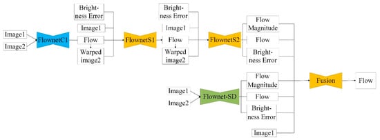
Figure 1.
Schematic diagram of the Flownet2 network structure.

Table 1.
RMSE (pixel) of some DLOF methods on the Sintel data set.
2.2. Compound Loss Function
2.2.1. RMSE Loss Function
The L2 function is also known as the mean square error function (MSE). As one of the most common loss functions in deep neural networks, it has excellent performance in super-resolution reconstruction, depth estimation, video frame interpolation, and other fields. However, for optical flow estimation, the L2 loss function does not have a clear physical meaning, making it difficult to establish an intuitive connection between the training of the model and the final prediction task. Therefore, in the deep learning optical flow estimation model, the root mean square error function (RMSE) obtained by taking the square root of the L2 function is usually used. The expression of RMSE is shown in Equation (1) below:
RMSE has a clear physical meaning in the optical flow estimation task: the modulus of the difference between the two vectors of the predicted value and the ground truth ω, that is, the Euclidean distance between the two.
2.2.2. AAE Loss Function
In the field of motion estimation, angular error is also a key parameter indicator. In the traditional method, the angle calculation is less directly put into the calculation model in the process of optimization calculation. Deep learning methods provide an end-to-end model of the task, which provides the basis for directly linking performance metrics from input data to output data. Therefore, the angular error can also be optimized as a loss function module of the deep learning method.
The error measure for displacement angle in the field of optical flow estimation proposed by the paper [26] is the average angular error (Average Angular Error), and its calculation method is given by the following Equation (2). The goal of AAE is to provide a relative performance measure to avoid the “divided by zero” problem of zero flow. In the AAE calculation, errors in large displacements are less punished than errors in small displacements; therefore, introducing AAE as a loss function can effectively improve the performance of small displacement estimation.
2.2.3. Div-Curl Smooth Loss Function
Curl and divergence are second-order physical quantities that describe the rotation and divergence characteristics of a space vector field. In flow field measurements, it establishes the connection between individual vectors and global vector flow field properties. Therefore, in this study, the curl and divergence of the true value of the flow field, and the curl and divergence of the predicted value of the model, are weighted by the second norm as the second-order flow field smoothing loss function, and the calculation equation is shown in Equation (3):
where represents the flow field vector, and are weighting coefficients, and = = 1 is selected in this study. The calculations of divergence and curl follow Equations (4) and (5):
2.2.4. Compound Form
Finally, the compound loss function consists of the above Equations (1)–(3). Its expression is given by Equation (6):
Due to the gradient propagation calculation characteristics of the deep learning method, in the process of minimizing the value of the loss function, the gradient backpropagation is passed layer by layer to update the model parameters of the entire network. For compound loss functions, a hyper parameter scale factor is often needed to adjust the connection of each loss function module. In order to enable each loss function module to play its due function, the order of magnitude of the calculation results of each module should be kept similar. According to the test of the training results of the separate RMSE loss function, the AAE error of the model is usually around 10°, while the RMSE error is below 1 pixel, and the average value of the curl and divergence is below 0.1. Therefore, this study uses RMSE as the basic loss function, and sets the value of the parameter to 1, the value of the parameter to 0.05, and the value of the parameter to 10. The specific sensitivity to parameter selection will be further analyzed in Section 3.3.
2.3. Synthetic PIV Data Set
The convolutional neural network is a supervised machine learning method, and the diversity of its training sample data set largely determines the generalization ability of the trained model to perform prediction or classification tasks. Therefore, in this study, a synthetic PIV data set is generated for model training and validation. The Flownet2 model with L2 loss function trained by the synthetic PIV data set is called Flownet2-PIV.
As shown in Figure 2, (a) and (b) are the former and transformed particle image pairs generated under the action of the flow field. In order to observe the fluid characteristics intuitively, (c) shows the vector drawn after sampling the flow field at intervals of 16 pixels. (d) is the palette used in the dense optical flow visualization process. Therefore, in the dense optical flow formatted image, the corresponding color area can be found on the palette according to the direction and size of the flow field. (e) shows the result of visualizing the dense flow field. Different colors represent different vector directions, and the brightness of the color represents the absolute value of the vector. (f) shows a schematic diagram of the flow field visualization that superimposes the dense visualization flow field and the sparse visualization flow field.
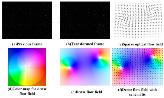
Figure 2.
Schematic diagram of dense optical flow PIV simulation data generation.
In order to make the PIV image data set more widely adaptable, this study generated the Hammel-Ossen vortex flow field, the Rankine vortex flow field, the linear flow field, the rotation flow field, and the membrane flow field. These five types of flow field models have different parameter variables, such as particle density distribution, sheet thickness, and maximum displacement. In the case of permutation and combination of parameters, a total of 9380 pairs of simulated images were generated, as shown in Table 2.
Table 2.
Setting of flow field type and maximum displacement parameter range.
The schematic diagram of the final generated flow field type is shown in Figure 3. In the subsequent experiments and analysis of this study, in order to correspond to the model parameters obtained by Flownet2 pre-training and reduce the image distortion caused by scaling, the height and width of the data set are 512 pixels × 384 pixels, respectively. The schematic diagram of the sparse flow field is drawn after sampling with a long and wide distribution interval of 16 pixels relative to the original flow field size, so as to observe the characteristics of the flow field.
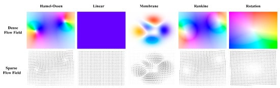
Figure 3.
Schematic diagram of flow field types.
3. Results and Analysis
3.1. Index of Performance Measurement
For the error analysis of the output flow field, from the perspective of physical quantities, the Euclidean distance error, angular error, curl, and divergence absolute error of the flow field vector are analyzed. Among them, the Euclidean distance error is the RMSE loss function used in Section 2, calculated by Equation (1). The angular error is calculated from the angle between the true value vector of the flow field and the predicted value, and its unit is converted into degrees (°). The calculation equation is obtained from the above Equation (2). As for the curl and divergence errors, because the curl and divergence of the two-dimensional vector field are scalar in the form of data representation, they are evaluated in the form of absolute errors. The calculation methods are as follows, in Equations (7) and (8).
3.2. Cosine Similarity Verification of Compound Loss Function
Gradient propagation of loss functions to model parameters is a core pattern in deep learning methods. Multiple target loss functions will generate corresponding model parameter gradients relatively independently. Tianhe Yu et al. [27]. proposed using cosine similarity to measure whether there is a competitive relationship between multiple tasks. If the loss function is regarded as , means the input data and output prediction data. Then, the gradient of the loss function can be expressed as dL/df. Since the FlowNet2 model has 1.6 × 10⁹ parameters, this gradient is usually a hyperdimensional vector. Similar to Formula (2) for calculating the cosine value of the angle between two vectors, Formula (9) can be used to measure the cosine similarity of two hyperdimensional vectors.
The value range of the cosine similarity is consistent with the value range of the cosine function, which is [−1, 1], and its value is also similar to the value of the cosine trigonometric function. The closer to 1, the more consistent the directions of the two are, and the closer to −1, the more inconsistent they are. Usually, if the cosine similarity of the loss function is less than 0, it indicates that there is a competitive relationship between the two optimization objectives, which is not conducive to the optimization of the model. Figure 4 shows the cosine similarity between pairs of compound loss functions proposed in this study.
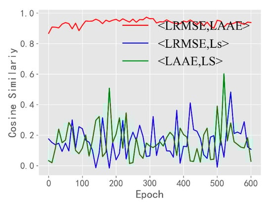
Figure 4.
Cosine similarity between parts of the compound loss function.
The experimental results show that there is a good cosine similarity between LRMSE and LAAE, while the cosine similarity between LS and LRMSE or LAAE is low but still over 0, which indicates that there is no confrontation between the tasks. This shows that all three parts of the compound loss function play a positive role in the optimization of the target task.
3.3. Sensitivity Analysis of Compound Loss Function Parameters
In Section 2.2, we propose using a compound loss function to optimize the training effect of the model. In this compound loss function, the parameter selection of the combination of each part still needs further discussion. However, the FlowNet2 model has more than 1.6 × 10⁹ model parameters, which adds difficulty to the training of the model. Therefore, in this part, we reduce the synthetic data set applied in Section 2.3 to 1/10, and verify the effect of parameter selection with a data set of about 1000 pairs of images. At the same time, because there are too few samples in the training data set, the final effect of the training is worse than the final result in Section 3.4. The purpose of this experiment is to compare the impact of different parameter choices on the model training effect. The experimental results are shown in Table 3 below.
Table 3.
Parameter Sensitivity Results of Compound Loss Functions on Limited Data Sets.
The experimental results show that the training effect of the model can be improved by focusing on LRMSE and adjusting each part to a similar order of magnitude. However, hyperparameter tuning of compound loss functions is still an issue that is difficult to fully discuss.
3.4. Results of Compound Form of Loss Function on Training Data Set
For the three parts of RMSE, AAE, and div-curl loss function in Section 2, Table 4 shows the test results of different combinations on the training set. It shows the impact of using only the LRMSE function and the various parts of the composite loss function on the large training effect. The parameter settings of the composite loss function are given in Section 2.2 and verified in Section 3.3. The experimental results show that incorporating the angular error into the loss function can not only improve the AAE accuracy of the final calculation result, but also improve the RMSE calculation accuracy to a certain extent. Combining the RMSE loss function with the div-curl loss function alone cannot achieve the desired effect. However, combining the three parts can achieve the best results in the three indicators of RMSE, AAE, and div-curl loss. This shows that curl and divergence, as measures of the local-global information of the flow field, do not contribute to the improvement of the calculation effect when the local information is not accurate enough, but when the single vector angle and amplitude errors are considered, the div-curl loss plays its part.
Table 4.
Results of different loss functions on the large training data set.
3.5. Analysis of RMSE Calculation Results
The RMSE results for each method are given in Figure 5. Five different types of flow fields are used in the simulated PIV data set generated in Section 4 of this study. Rigid body motion usually has the characteristics of regional consistency, brightness invariance, etc., which are similar to the characteristics of the linear flow field and the large vortex field in the PIV data set, and both have a wide range of change rates. However, the Hamel-Ossen type and Rankine vortex flow fields contain large displacement amplitude, gradient convective flow, small displacement, and large angle change vortex center characteristics, which are relatively rare in rigid body motion. Different flow field models fields characterize the complexity of fluid motion characteristics and, in the two model methods that also use fluid data set training, the Flownet2-CL-PIV method combined with the compound loss function estimates various flow field types. Accuracy is achieved better than with training methods using the traditional L2 loss function.
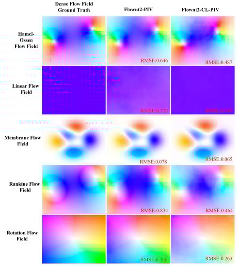
Figure 5.
RMSE results of two methods on different flow fields.
3.6. Analysis of AAE Calculation Results
At the angular error level, since the L2 loss function is actually a manifestation of the Euclidean distance for a single vector, using the L2 loss function can theoretically optimize the estimated vector that coincides with the original vector, which can also reduce the error of the angle. However, when the calculation result is not 100% accurate, there will be multiple different vector calculations to obtain the same angular error at the same Euclidean distance error. So, as shown in Figure 6, the model using the L2 loss function will have poor results in the angular error.
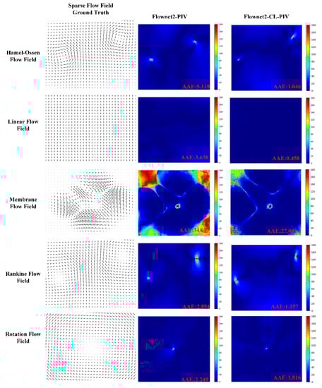
Figure 6.
AAE results of two methods on different flow fields.
3.7. Analysis of Div-Curl Error Calculation Results
The curl and divergence of a vector field are usually physical quantities used in fluid estimation. Figure 7 shows the calculation results of the curl and divergence errors using the Hamel-Ossen type flow field with a large displacement variation range and a large angle variation range as an example. Similar to the calculation results of RMSE and AAE, the errors of curl and divergence are also concentrated in the central part of the vortex. However, the training model using the compound loss function has the smallest error in the characteristics of the second-order flow field, and better retains the overall physical characteristics of the flow field.
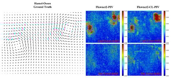
Figure 7.
Div-curl error of two methods on the Hamel-Ossen flow field.
4. Conclusions
In this study, a compound loss function combining RMSE loss, angular error loss, and div-curl loss is introduced into the deep learning optical flow estimation method Flownet2 model, and the Flownet2-CL-PIV method is proposed. For the training of the deep learning model and the performance analysis of the calculation results, this study chooses the method of generating synthetic particle images. The particle image generated in this study contains five different flow models, reflecting the characteristics of fluid flow that are different from rigid body motion: the displacement and angle distribution range is large, the amplitude distribution is continuous, and the vortex center has small displacement amplitude and large angle change. On the basis of synthetic simulation data sets, this study compares the computational accuracy of the Flownet2-PIV and Flownet2-CL-PIV models using the traditional L2 loss function in terms of RMSE, AAE, and div-curl.
The results of simulation experiments show that: (1) The AAE loss function can be improved in the final calculation index, while div-curl loss cannot achieve the corresponding effect when combined with RMSE loss function alone, but the combination of the three can achieve the best effect. (2) In fluid motion estimation, the errors are mainly concentrated in areas with large angular gradients and small displacement amplitudes, such as vortex centers and seepage boundaries. (3) Through the measurement of cosine similarity, it is demonstrated that each part of the composite loss function proposed in this paper optimizes the task from different angles. In addition, keeping each part of the composite loss function at a similar order of magnitude is helpful for target optimization. (4) Compared with the L2 loss function, the compound loss function proposed in this paper can obtain the flow field with smaller direction and distance estimation errors, and retain more global curl-divergence information of the flow field, which is fine, and small-scale fluid motion structure observations provide support.
However, the use of compound loss functions also leads to the following problems: (1) It is difficult to fully discuss the selection of hyperparameters, making it difficult to obtain the most effective value range of these parameters. (2) The compound loss function also makes the parameter optimization of the model more complicated, and it is difficult to achieve the global optimal solution of the model.
Therefore, in the next stage of work, we plan to adopt a compound loss function that can learn parameters to avoid the uncertainty caused by manual parameter adjustment. For the application of the DLOF method in the field of PIV, the characteristics of fluid motion should be further studied. Whether at the structure level of the neural network model or the level of the loss function, a proper description of the fluid motion characteristics can achieve better results in the application of the method.
Author Contributions
Conceptualization, J.W. and Z.Z.; methodology, J.W. and Z.Z.; software, J.W.; validation, L.C. and Z.W.; resources, Z.Z.; writing—original draft preparation, J.W.; writing—review and editing, Z.Z. and Z.W. All authors have read and agreed to the published version of the manuscript.
Funding
This work was supported by the China Postdoctoral Science Foundation (No. 2019M651673), the Fundamental Research Funds for the Central Universities (No. B200202187) and Jiangsu Water Conservancy Science and Technology Project (No.2021070).
Data Availability Statement
All data included in this study are available upon request by contact with the corresponding author.
Conflicts of Interest
The authors declare no conflict of interest.
References
- Raffel, M.; Willert, C.; Wereley, S.; Kompenhans, J. Particle Image Velocimetry: A Practical Guide; Springer: Cham, Switzerland, 2007. [Google Scholar]
- Cai, S. Optical Flow-Based Motion Estimation of Complex Flows; Zhejiang University: Hangzhou, China, 2019. [Google Scholar]
- Wang, J.; Shi, T.; Yu, D.; Teng, D.; Ge, X.; Zhang, Z.; Yang, X.; Wang, H.; Wu, G. Ensemble machine-learning-based framework for estimating total nitrogen concentration in water using drone-borne hyperspectral imagery of emergent plants: A case study in an arid oasis, NW China. Environ. Pollut. 2020, 266, 115412. [Google Scholar] [CrossRef] [PubMed]
- Shinohara, K.; Sugii, Y.; Aota, A.; Hibara, A.; Tokeshi, M.; Kitamori, T.; Okamoto, K. High-Speed Micro PIV Measurements of Micro Counter-Current Flow. Proc. JSME Annu. Meet. 2004, 2004, 111–112. [Google Scholar] [CrossRef]
- Westerweel, J. Digital Particle Image Velocimetry: Theory and Application. Ph.D. Thesis, Delft University, Delft, The Netherlands, 1995. [Google Scholar]
- Scarano, F.; Riethmuller, M.L. Iterative Multigrid Approach in PIV Image Processing with Discrete Window Offset. Exp. Fluids 1999, 26, 513–523. [Google Scholar] [CrossRef]
- Horn, B.; Schunck, B. Determining optical flow. Artif. Intell. 1981, 17, 185–203. [Google Scholar] [CrossRef]
- Corpetti, T.; Memin, E.; Perez, P. Dense Estimation of Fluid Flows. Pattern Anal. Mach. Intell. IEEE Trans. 2002, 24, 365–380. [Google Scholar] [CrossRef]
- Liu, T.S.; Shen, L.X. Fluid flow and optical flow. J. Fluid Mech. 2008, 614, 253–291. [Google Scholar] [CrossRef]
- Tauro, F.; Tosi, F.; Mattoccia, S.; Toth, E.; Piscopia, R.; Grimaldi, S. Optical Tracking Velocimetry (OTV): Leveraging Optical Flow and Trajectory-Based Filtering for Surface Streamflow Observations. Remote Sens. 2018, 10, 2010. [Google Scholar] [CrossRef]
- Khalid, M.; Pénard, L.; Mémin, E. Optical flow for image-based river velocity estimation. Flow Meas. Instrum. 2019, 65, 110–121. [Google Scholar] [CrossRef]
- Hui, T.W.; Tang, X.; Loy, C.C. LiteFlowNet: A Lightweight Convolutional Neural Network for Optical Flow Estimation. In Proceedings of the 2018 IEEE/CVF Conference on Computer Vision and Pattern Recognition, Salt Lake City, UT, USA, 18–23 June 2018. [Google Scholar]
- Fischer, P.; Dosovitskiy, A.; Ilg, E.; Häusser, P.; Hazırbaş, C.; Golkov, V.; Van der Smagt, P.; Cremers, D.; Brox, T. FlowNet: Learning Optical Flow with Convolutional Networks. In Proceedings of the 2015 IEEE International Conference on Computer Vision (ICCV), Santiago, Chile, 7–13 December 2015. [Google Scholar]
- Sun, D.; Yang, X.; Liu, M.Y.; Kautz, J. PWC-Net: CNNs for Optical Flow Using Pyramid, Warping, and Cost Volume. In Proceedings of the 2018 IEEE/CVF Conference on Computer Vision and Pattern Recognition (CVPR), Salt Lake City, UT, USA, 18–23 June 2018. [Google Scholar]
- Teed, Z.; Deng, J. RAFT: Recurrent All-Pairs Field Transforms for Optical Flow; Springer: Berlin/Heidelberg, Germany, 2020. [Google Scholar]
- Ilg, E.; Mayer, N.; Saikia, T.; Keuper, M.; Dosovitskiy, A.; Brox, T. FlowNet 2.0: Evolution of Optical Flow Estimation with Deep Networks. In Proceedings of the IEEE Conference on Computer Vision and Pattern Recognition (CVPR), Honolulu, HI, USA, 21–26 July 2017. [Google Scholar]
- Lee, Y.; Yang, H.; Yin, Z. PIV-DCNN: Cascaded deep convolutional neural networks for particle image velocimetry. Exp. Fluids 2017, 58, 171. [Google Scholar] [CrossRef]
- Kondor, S.; Chan, D.; Sitterle, J. Application of Optical Surface Flow Measurement to Composite Resin Shrinkage. In Proceedings of the ADEA/AADR/CADR Meeting & Exhibition, Orlando, FL, USA, 8–9 March 2006. [Google Scholar]
- Cai, S.; Liang, J.; Gao, Q.; Xu, C.; Wei, R. Particle Image Velocimetry Based on a Deep Learning Motion Estimator. IEEE Trans. Instrum. Meas. 2020, 69, 3538–3554. [Google Scholar] [CrossRef]
- Cai, S.; Zhou, S.; Xu, C.; Gao, Q. Dense motion estimation of particle images via a convolutional neural network. Exp. Fluids 2019, 60, 73. [Google Scholar] [CrossRef]
- Dickson, M.C.; Bosman, A.S.; Malan, K.M. Hybridised loss functions for improved neural network generalization. In Proceedings of the Pan-African Artificial Intelligence and Smart Systems: First International Conference, PAAISS 2021, Windhoek, Namibia, 6–8 September 2021; Springer International Publishing: Cham, Switzerland, 2022; pp. 169–181. [Google Scholar]
- Kendall, A.; Gal, Y.; Cipolla, R. Multi-task learning using uncertainty to weigh losses for scene geometry and semantics. In Proceedings of the IEEE Conference on Computer Vision and Pattern Recognition 2018, Salt Lake City, UT, USA, 18–22 June 2018; pp. 7482–7491. [Google Scholar]
- Sener, O.; Koltun, V. Multi-task learning as multi-objective optimization. Adv. Neural Inf. Process. Syst. 2018, 31, 1–12. [Google Scholar]
- Yu, C.D.; Fan, Y.W.; Bi, X.J.; Han, Y.; Kuai, Y.F. Deep particle image velocimetry supervised learning under light conditions. Flow Meas. Instrum. 2021, 80, 102000. [Google Scholar] [CrossRef]
- Yu, C.; Luo, H.; Fan, Y.; Bi, X.; He, M. A cascaded convolutional neural network for two-phase flow PIV of an object entering water. IEEE Trans. Instrum. Meas. 2021, 71, 1–10. [Google Scholar] [CrossRef]
- Baker, S.; Scharstein, D.; Lewis, J.P.; Roth, S.; Black, M.J.; Szeliski, R. A Database and Evaluation Methodology for Optical Flow. Int. J. Comput. Vis. 2011, 92, 1–31. [Google Scholar] [CrossRef]
- Yu, T.; Kumar, S.; Gupta, A.; Levine, S.; Hausman, K.; Finn, C. Gradient surgery for multi-task learning. Adv. Neural Inf. Process. Syst. 2020, 33, 5824–5836. [Google Scholar]


Disclaimer/Publisher’s Note: The statements, opinions and data contained in all publications are solely those of the individual author(s) and contributor(s) and not of MDPI and/or the editor(s). MDPI and/or the editor(s) disclaim responsibility for any injury to people or property resulting from any ideas, methods, instructions or products referred to in the content. |
© 2023 by the authors. Licensee MDPI, Basel, Switzerland. This article is an open access article distributed under the terms and conditions of the Creative Commons Attribution (CC BY) license (https://creativecommons.org/licenses/by/4.0/).