Abstract
The calculation of erosion and deposition in riverways plays a pivotal role in river morphology studies, comprehensive river management and flood safety. Some existing methods have certain limitations in terms of accuracy and applicability. To address these challenges, we propose a method for calculating riverway erosion and deposition based on measured cross-sectional terrain data. This method not only enables the calculation of changes in erosion and deposition along the riverway but also provides information on the spatial distribution of these changes. The validity of the proposed calculation method was assessed using measured bathymetric data. The results indicate a relative error of only 5.6% between the calculated and measured values for the total volume of erosion and deposition. A comparison with the results obtained using a cross-section method reveals that, with an average distance between adjacent sections of 1.0 km, the proposed method generally outperforms the cross-section method. The relative error in the total volume of erosion and deposition decreases from 19.2% with the cross-sectional method to 5.6% with our proposed method. When facing the need to calculate changes in riverway erosion and deposition, our approach offers a more accurate and flexible computational method.
1. Introduction
The calculation of erosion and deposition in riverways plays a pivotal role in studying river morphology, performing comprehensive river management and ensuring flood safety [1,2]. The erosion and deposition conditions are critical indicators for assessing the stability and safety of rivers, serving as essential bases for formulating river management and planning strategies [3,4,5].
Currently, there are numerous methods for calculating riverway erosion and deposition. For instance, Azarang et al. [6] simulated the erosion and deposition downstream of the Karkheh reservoir dam before construction using the MIKE11 model. Adib et al. [7] employed the Fluvial-12 model to compute erosion and deposition changes in the Karun River in Iran. However, the two most widely used methods are the sediment transport rate method and the cross-section method [8,9,10]. The sediment transport rate method involves calculating erosion and deposition based on measured sediment transport data at the inlet and outlet hydrological stations of a reach [11]. Due to the continuous nature of sediment data collection at hydrological stations, it can reflect the variations in erosion and deposition processes along the entire studied reach. However, the sediment transport rate method can only reveal the total volume of erosion and deposition over a long river segment between two hydrological stations [12]. It cannot capture along-riverway variations in erosion and deposition between the two stations. Moreover, the distance between two hydrological stations is typically long in actual rivers [13], making this method unsuitable for short river segments. Additionally, due to the current limitations in sediment transport data measurement technology, the measurement of sediment concentration is often influenced by the measurement point selection and sampling depth, resulting in low measurement accuracy and introducing errors into the calculation results [14]. Furthermore, these errors gradually accumulate over time. Importantly, this method, as it cannot account for changes in erosion and deposition caused by bedload transport, is only applicable to rivers where suspended sediment transport is predominant.
Simultaneously, in order to investigate the evolution of river erosion and deposition, it is common to set up fixed-observation cross-sections at regular distances along the river. With the terrain data from these observed cross-sections as a foundation, the cross-section method becomes a viable approach to calculating the erosion and deposition in a riverway. This method approximates the river reach between two measured cross-sections as a truncated cone. The areas of flow for the two cross-sections are treated as the two cross-sectional areas of the truncated cone. The distance between the two measured cross-sections serves as the length of the truncated cone. The volume of the truncated cone represents the channel storage volume [15,16]. The difference in the calculated channel storage volumes between the two instances corresponds to the erosion and deposition volume. For instance, Liu et al. [17] used the cross-section method to calculate the changes in riverbed erosion and deposition in the Lower Yellow River from 1965 to 2014 to study the impact of riverbed and floodplain changes on water and sediment conditions. Xia et al. [18] applied the cross-section method to calculate sediment erosion and deposition in the middle and lower reaches of the Yangtze River since the completion of the Three Gorges Project, supporting channel management and basin sediment management. Yuan et al. [19] used the cross-section method to study the trends in riverbed topographic changes in the Ningxia Plain Reaches of the Yellow River, calculating sediment erosion and deposition at different time periods and their variations. Lyu et al. [20] used the cross-section method to investigate riverbed changes in the middle reaches of the Yangtze River from Yichang to Chenglingji, providing insights into the impact of the Three Gorges Project on downstream riverbed morphodynamic adjustments. However, through the analysis of the aforementioned research outcomes, we identified some shortcomings in employing the cross-section method for riverway erosion and deposition calculations. Firstly, it fails to reflect the meandering morphology of rivers since it directly connects two cross-sections with a straight line when conceptualizing the truncated cone. Natural rivers are typically not straight, leading to potential calculation errors [21,22]. Secondly, it does not depict the spatial distribution of erosion and deposition changes along the calculated riverway. The cross-section method calculates the erosion and deposition between adjacent cross-sections and accumulates these values to obtain the total erosion and deposition volume for the entire riverway [23]. However, understanding the distribution of erosion and deposition is crucial for studying river channel changes. This can provide a basis for targeted management measures for river managers.
Based on this, this paper proposes a method for calculating riverway erosion and deposition based on measured cross-sectional terrain data. This method is designed for the computation of riverway erosion and deposition. It not only considers the meandering morphology of rivers by introducing auxiliary lines, such as river boundaries and water edges, but also incorporates a quadrilateral grid to obtain the spatial distribution of erosion and deposition changes in the riverway. In comparison to the cross-section method, this approach can provide more accurate calculation results and offer information about the spatial distribution of erosion and deposition changes that the cross-section method cannot provide.
2. Riverway Erosion and Deposition Calculation Method
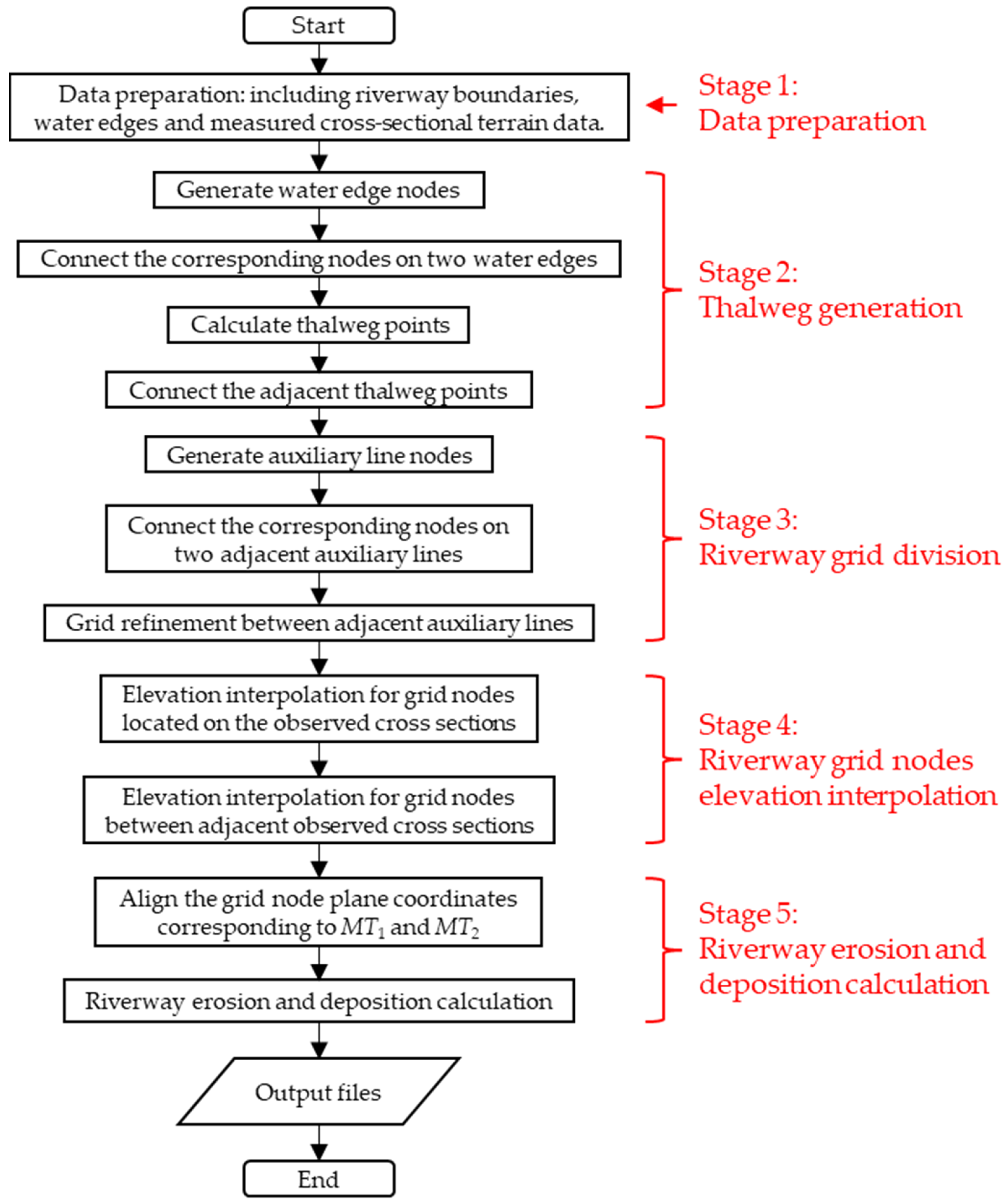
For a river segment requiring the calculation of erosion and deposition changes, based on cross-sectional terrain data measured at two different times, the following steps can be employed to calculate the erosion and deposition variations (designated as MT1 and MT2 for the first and second measurement times, respectively). Firstly, the riverway boundaries and water edges corresponding to MT1 and MT2 are utilized as auxiliary lines to create two sets of quadrilateral grids. Subsequently, the elevation information for all nodes on these two grids is calculated using the cross-sectional terrain data obtained at MT1 and MT2. Finally, the erosion and deposition conditions of the target river segment during the MT1–MT2 period are determined using the two sets of grids corresponding to MT1 and MT2. The elevation of any point within the riverbed is influenced by the measured cross-sectional terrain data of its two adjacent measured sections. The entire river segment can be subdivided into multiple sub-segments using the observed cross-sections. These sub-segments share a consistent calculation method, illustrating that one sub-segment serves as an example. The detailed process can be roughly divided into the following five stages (see Figure 1):

Figure 1.
Riverway erosion and deposition calculation process.
Stage 1—Data preparation: The planar coordinate data for the boundaries on both sides of the riverway corresponding to MT1 and MT2, as well as the planar coordinate data for the left and right water edges corresponding to MT1 and MT2 and the measured cross-sectional terrain data corresponding to MT1 and MT2, must be prepared in advance.
Stage 2—Thalweg generation: The planar coordinate data for the left and right water edges corresponding to MT1 and MT2 and the measured cross-sectional terrain data corresponding to MT1 and MT2 are used to calculate the thalweg for the respective measurement times.
Stage 3—Riverway grid division: By incorporating the riverway boundaries, water edges and thalweg as auxiliary lines, quadrilateral grids corresponding to MT1 are generated on the target river segment, effectively reflecting the course of the riverway. Similarly, quadrilateral grids corresponding to MT2 are obtained.
Stage 4—Riverway grid node elevation interpolation: Measured cross-sectional terrain data corresponding to MT1 and MT2 are interpolated onto the grid nodes located on the measured cross-sections using distance-weighted interpolation methods. Subsequently, distance-weighted interpolation methods are employed in the water flow direction to obtain elevation information for all grid nodes between the two measured cross-sections.
Stage 5—Riverway erosion and deposition calculation: The planar coordinates of the two sets of grids are matched and calculated with node elevation data corresponding to MT1 and MT2. The erosion and deposition volume and spatial distribution between the two measured cross-sections during the MT1–MT2 period are determined.
2.1. Data Preparation
Before commencing the calculations, the cross-sectional terrain data corresponding to MT1 and MT2, the planar coordinate data for the boundaries on both sides of the riverway corresponding to MT1 and MT2, and the planar coordinate data for the water edges on both sides of the riverway corresponding to MT1 and MT2 need to be prepared.
2.2. Thalweg Generation
In order to make the generated quadrilateral grids better adapt to the course of the river and changes in the terrain, water edges and the thalweg are introduced as auxiliary lines in the grid generation process, in addition to the riverway boundaries. The riverway boundaries and water edges can be obtained through field measurements or by interpreting remote sensing images [24,25,26,27]. In contrast, obtaining the thalweg can be more challenging. Thalwegs are submerged beneath the water and are generally difficult to directly obtain. Field measurements of thalwegs can be labor-intensive and resource-intensive. Here, we propose a method for determining the thalweg using water edges and measured cross-sectional terrain data, with an example focused on the subsection between measured cross-sections c and c + 1. Furthermore, in accordance with the conventions of river hydrodynamics, we define the left side as the left bank and the right side as the right bank when facing the water flow; this convention will be consistently followed.
The left and right water edges are equally divided into N segments by length [28], resulting in nodes along the left and right water edges, denoted by and , where i = 1,2,3,…, N + 1 (see Figure 2a). In fact, the value of N should be appropriately selected based on the distance between the two measured cross-sections. A larger N results in a smoother thalweg, but it also leads to a higher computational workload. Points at the corresponding positions of the left and right water edges are sequentially connected to form N + 1 subsections (see Figure 2b). Subsequently, a dimensionless parameter, denoted by T, is introduced to represent the deviation of the thalweg point between the two water edges, calculated using Equation (1). The T values range between 0 and 1, with values closer to 0 indicating that the thalweg point is closer to the left water edge and values closer to 1 indicating proximity to the right water edge. The T values, T(c) and T(c + 1), are computed separately for cross-sections c and c + 1.
where represents the horizontal distance of the thalweg point from the left endpoint of the observed cross-section, denotes the horizontal distance of the left water edge from the left endpoint of the observed cross-section, and represents the horizontal distance of the right water edge from the left endpoint of the observed cross-section.
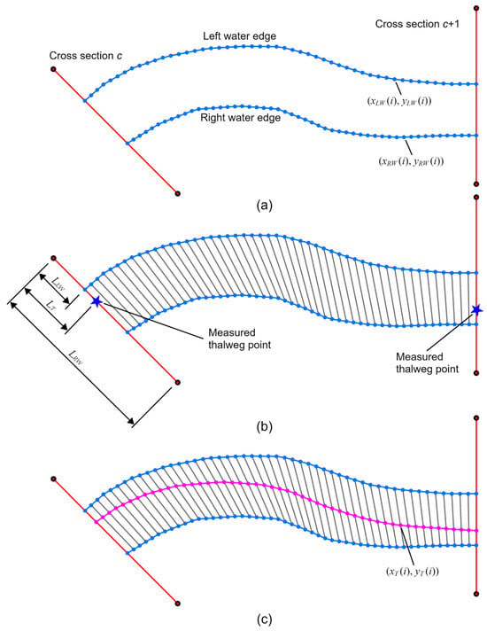
Figure 2.
Generation of the thalweg. (a) Node generation of water edges; (b) T number calculation; (c) Node generation of thalweg.
Subsequently, interpolation is employed according to Equation (2) to calculate the T values, T(i), for all N + 1 subsections between the two observed cross-sections. Based on the T values for each subsection and the planar coordinates, and , of their left and right endpoints, the planar coordinates of each thalweg point, denoted by , are computed using Equations (3) and (4), where i = 1,2,3,…, N + 1. Subsequently, the generated thalweg points are sequentially connected to form the thalweg, as illustrated in Figure 2c.
2.3. Riverway Grid Division
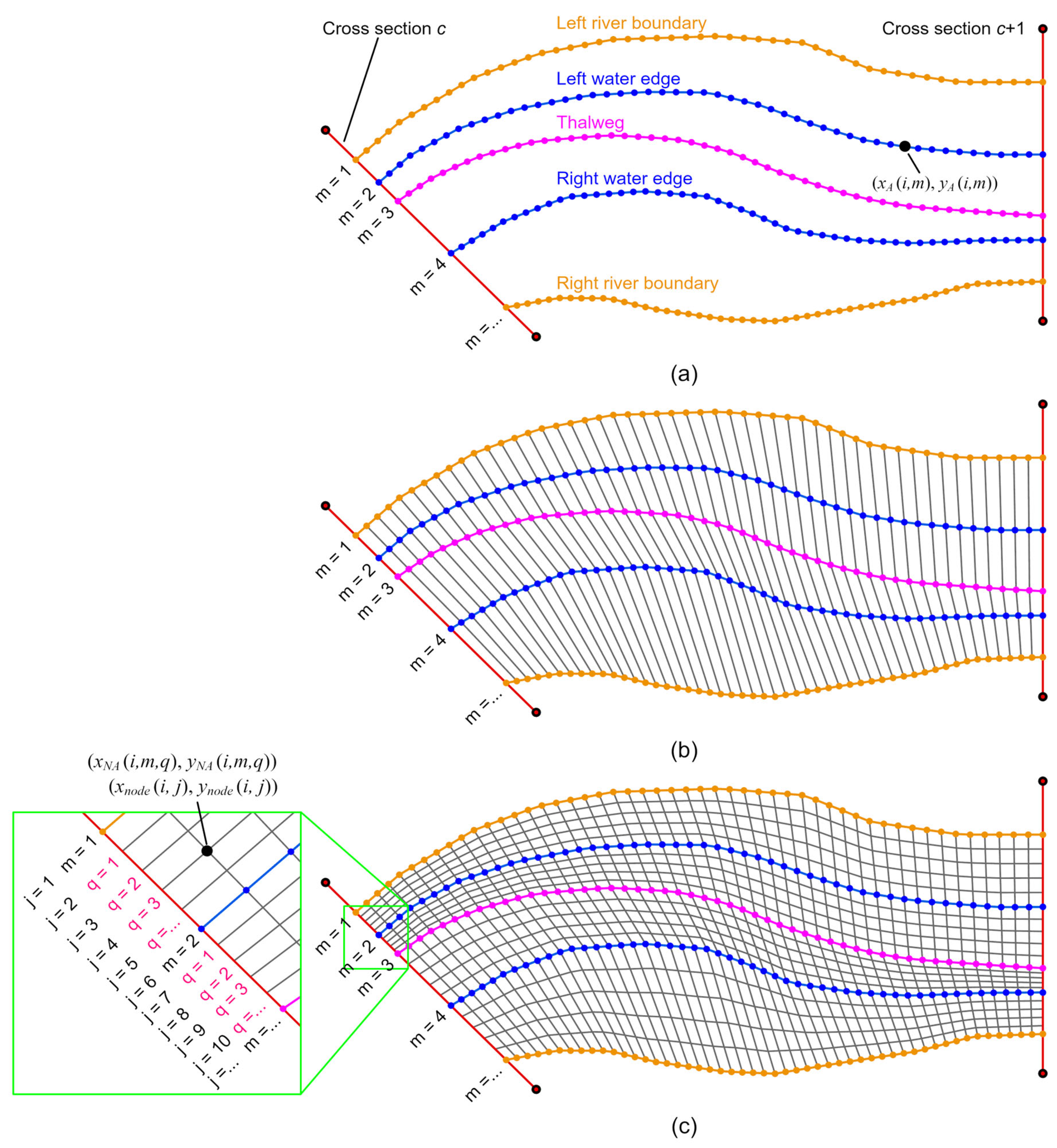
In the process of subdividing the target riverway using quadrilateral grids, auxiliary lines such as the riverway boundaries, water edges and thalweg are introduced, assuming that there are a total of M such auxiliary lines. Each of these auxiliary lines is equally divided into N segments by length. The coordinates of the ith node on the mth auxiliary line are denoted by , where i = 1, 2, 3, …, N + 1, and m = 1, 2, 3, …, M (see Figure 3a). Subsequently, nodes with the same index on adjacent auxiliary lines, and , are connected in sequence, resulting in a preliminary grid, as shown in Figure 3b. It is evident that a grid subdivided in this manner exhibits relatively large spacing between the two auxiliary lines, which significantly impacts the accuracy of the computation results. Therefore, refinement is required in the region between the two auxiliary lines. Here, we divide the lines connecting corresponding nodes on every two auxiliary lines into Q segments. Of course, the number of segments between different pairs of auxiliary lines may vary and can be adjusted based on actual distances to ensure a uniform grid density across the entire region. The new grid nodes between two auxiliary lines can be calculated using Equations (5) and (6), where i = 1, 2, 3, …, N + 1; q = 1, 2, 3, …, Q − 1; and m = 1, 2, 3, …, M − 1 (see Figure 3c). For ease of programming, the arrays and are reduced in dimensionality. The nodes on the auxiliary lines are also included. This results in a restructured set of coordinates for all grid nodes, denoted by , as shown in Figure 3c, where i = 1, 2, 3, …, N + 1; j = 1, 2, 3, …, J; and J = 1+.
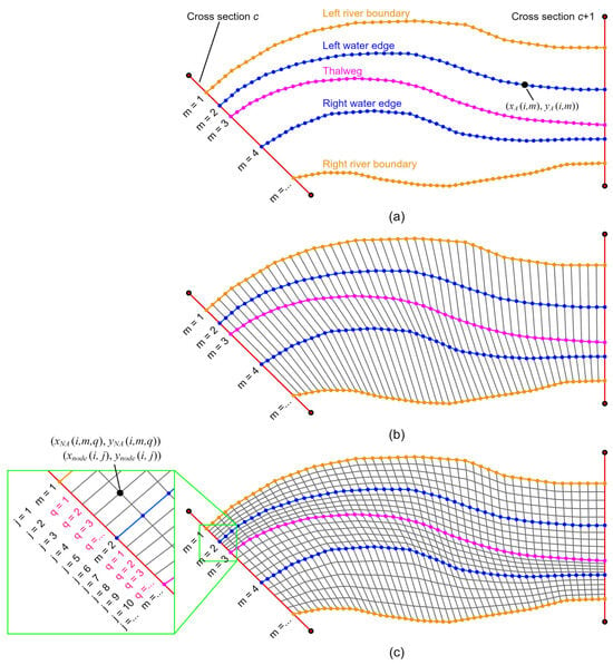
Figure 3.
Schematic diagram of river channel grid division. (a) Node generation of auxiliary lines; (b) Generation of preliminary grid; (c) Refinement of preliminary grid.
2.4. Riverway Grid Node Elevation Interpolation
Interpolating the actual cross-sectional terrain data to the grid nodes involves two steps: firstly, interpolating the actual cross-sectional terrain data to the grid nodes located on the observed cross-sections; secondly, using the distance between adjacent observed cross-sections as weights and calculating the elevations for all grid nodes between two observed cross-sections. The specific steps are as follows:
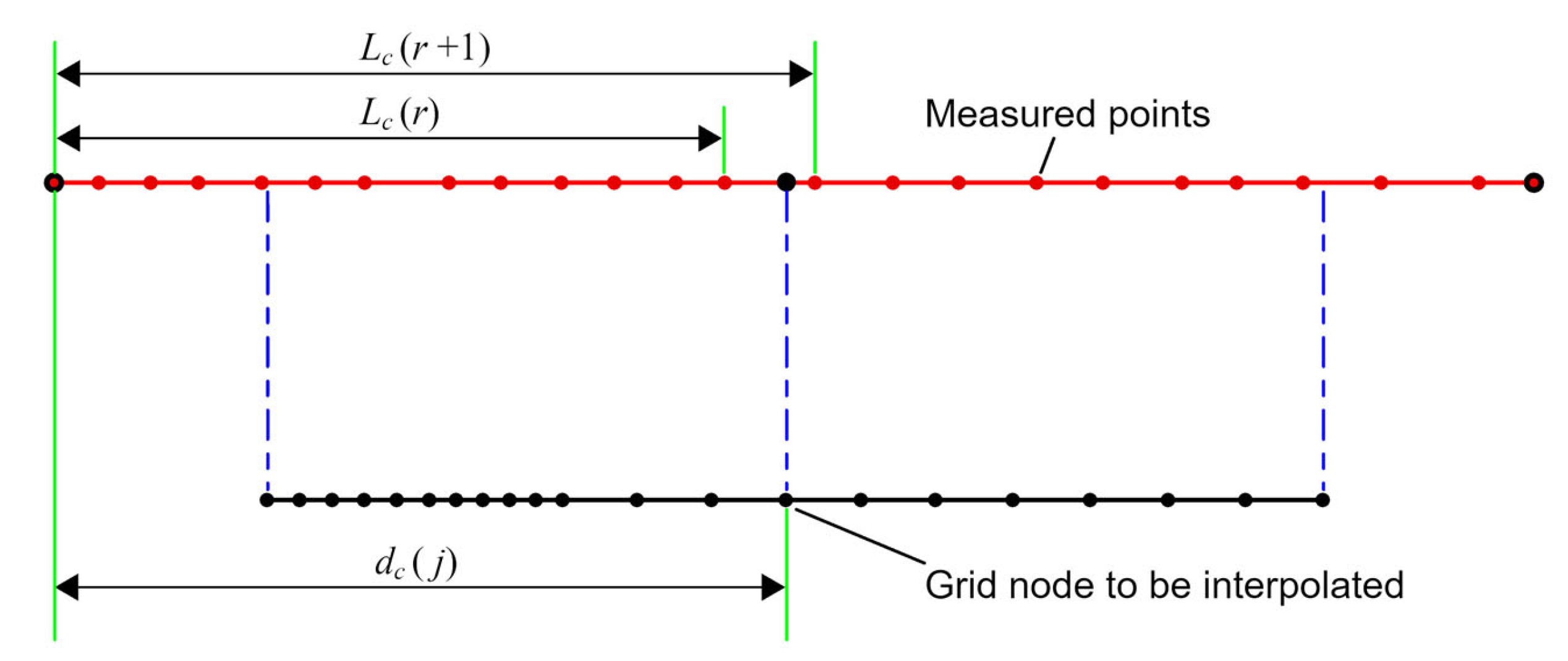
Step 1: Elevation interpolation for grid nodes located on the observed cross-sections. For each grid node located on the observed cross-section c, its horizontal distance to the left endpoint can be calculated using Equation (7). Similarly, for each grid node located on the observed cross-section c + 1, its horizontal distance to the left endpoint can be calculated using Equation (8). For any grid nodes located on cross-section c, if falls between the horizontal distances of the two observed points on cross-section c, namely, , the elevation can be calculated using Equation (9) according to the two corresponding measured elevation values and (see Figure 4). Similarly, the elevation can be calculated for grid nodes located on cross-section c + 1.
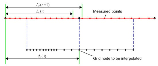
Figure 4.
Elevation interpolation for grid nodes located on the observed cross-sections.
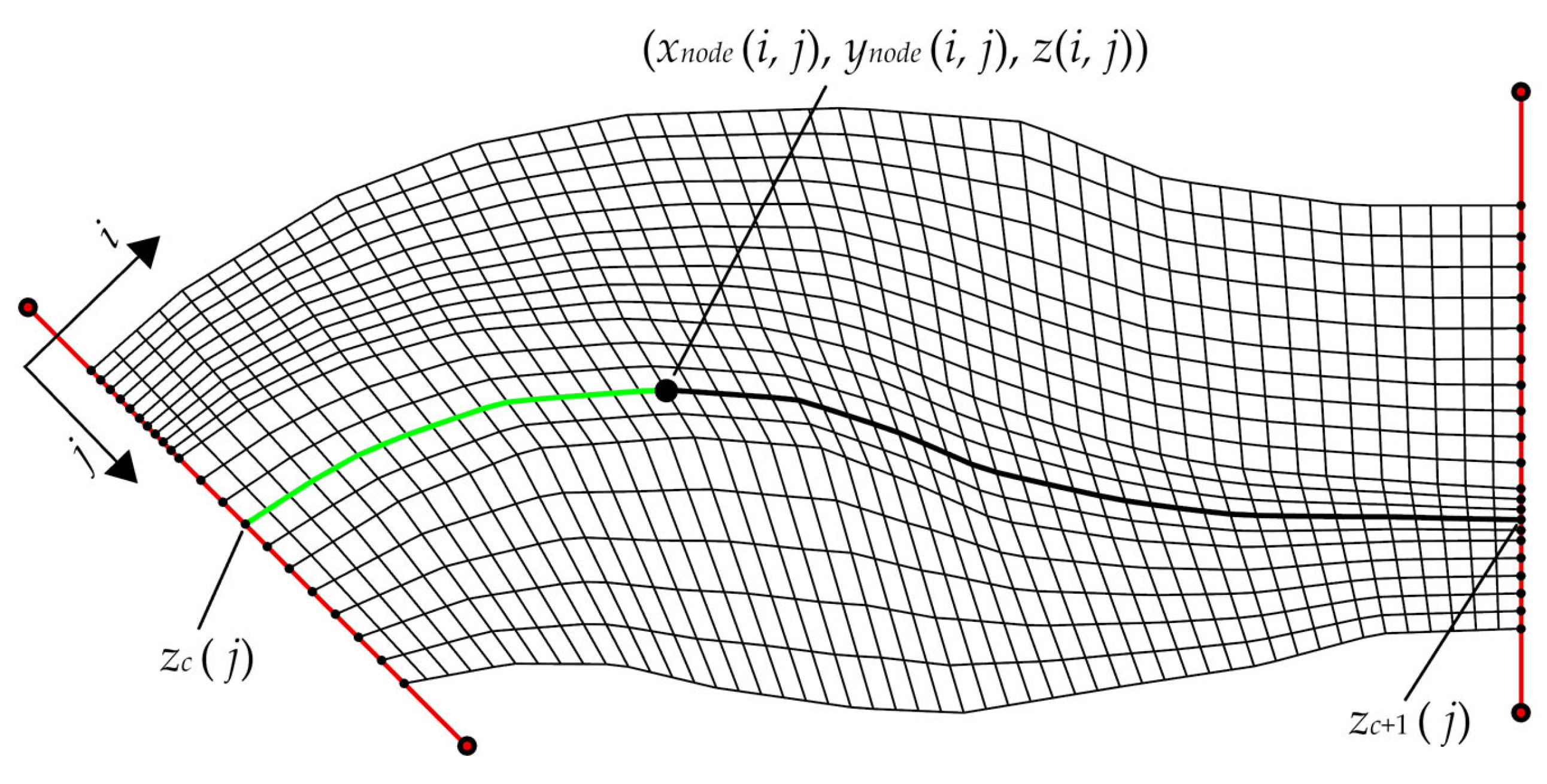
Step 2: Elevation interpolation for grid nodes between adjacent observed cross-sections. The cumulative distances from each grid node located on every longitudinal (in the flow direction) grid line to cross-section c are computed. The cumulative distance for the first grid node on each longitudinal grid line to cross-section c is set to zero, while for the subsequent nodes, it is calculated using Equation (10). In essence, the cumulative distance for the last grid node on each longitudinal grid line is equivalent to the total length of that particular longitudinal grid line (Figure 5). Subsequently, the cumulative distances of the target interpolation grid nodes to both observed cross-sections are employed as weights, using Equation (11) to interpolate and calculate their elevation values .

Figure 5.
Elevation interpolation for grid nodes between adjacent observed cross-sections.
2.5. Riverway Erosion and Deposition Calculation
Using the aforementioned methods, we obtain the coordinates of the grid nodes, with corresponding to MT1 and corresponding to MT2. Due to the differing positions of the water edges for MT1 and MT2, the location of the thalweg naturally exhibits some variation. While the generated grids have the same number of rows and columns, the planar coordinate positions of the grid nodes differ somewhat. To calculate the elevation change for grid nodes corresponding to MT1 and MT2, it is necessary to align the planar coordinates of the nodes from these two sets of grids by means of interpolation. This enables the direct calculation of the elevation difference for the corresponding nodes. The specific procedure involves interpolating the grid nodes corresponding to MT1 onto the grid nodes corresponding to MT2, yielding the grid node coordinates . A four-point natural neighbor interpolation method is employed for this purpose. In essence, this method selects the four closest points, , , and , from the grid nodes corresponding to MT1 to the target point based on their planar Euclidean distances , , and to the target point. Subsequently, the elevation at the target point can be calculated as per Equation (12). Furthermore, the change in riverbed elevation at each grid node can also be calculated using Equation (13). If , the node exhibits erosion; if , the node indicates deposition; if , the node remains unchanged. The distribution of erosion and deposition in the entire sub-river segment is illustrated in Figure 6.
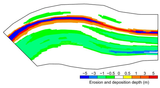
Figure 6.
The distribution of erosion and deposition in the entire sub-river segment.
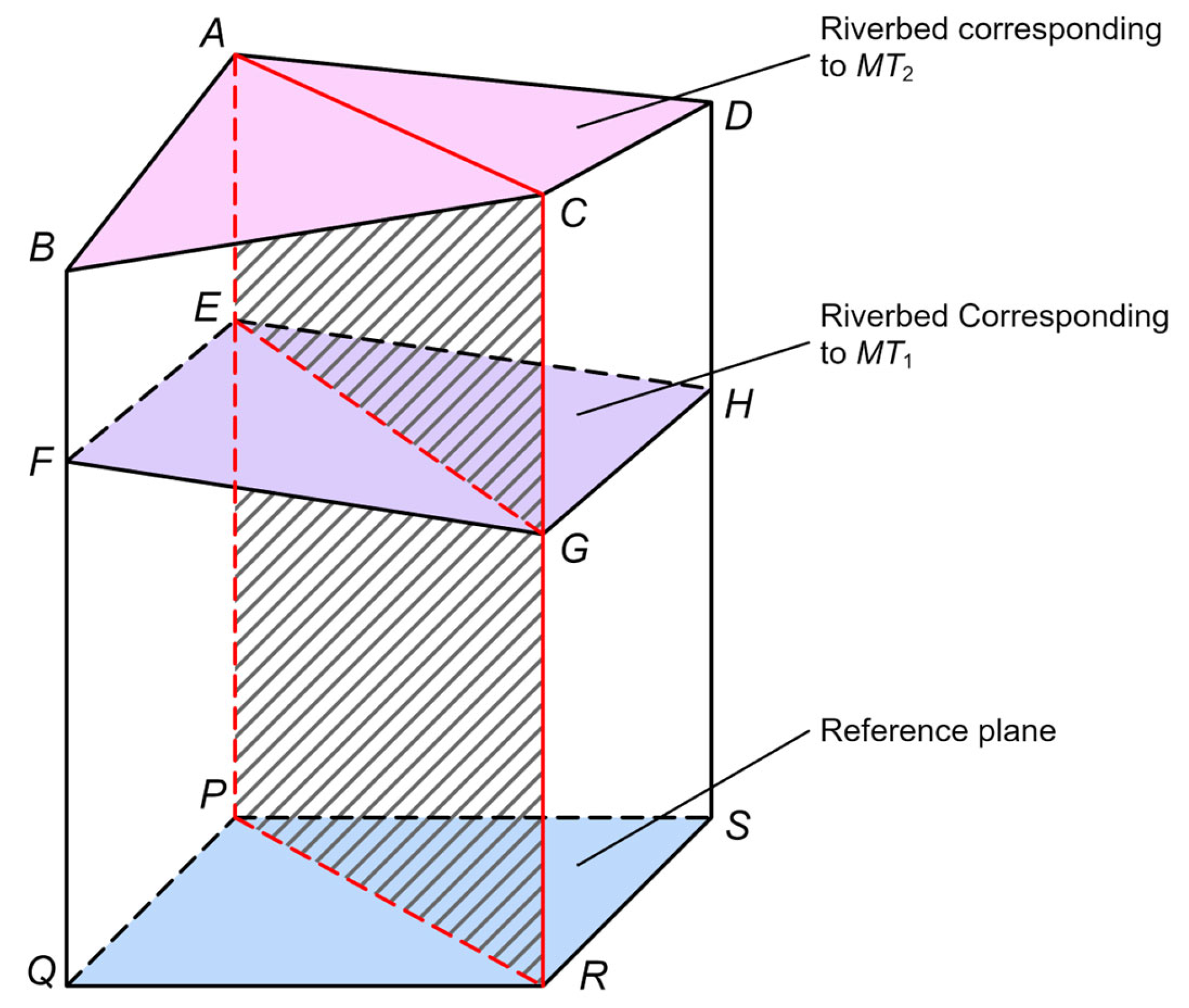
As the plane coordinates of the grid nodes corresponding to MT1 and MT2 have already been aligned, the calculation element for sediment erosion and deposition, denoted by ABCDEFGH in Figure 7, is defined by its eight vertices, whose coordinates are listed in Table 1. This unit represents a polyhedron with four vertices, A, B, C and D, corresponding to the bed elevations of MT2, and four vertices, E, F, G and H, representing the bed elevations of MT1. The volume of this polyhedron, denoted by ABCDEFGH, represents the sediment volume change within this calculation element. Since the vertices A, B, C and D may not lie in the same plane, the vertices E, F, G and H may not be coplanar, and it is necessary to further divide this polyhedron into two triangular prisms, ABCEFG and ACDEGH. Taking the polyhedron ABCEFG as an example, the upper-surface vertices A, B and C are reordered according to their node elevations in ascending order, resulting in the sequence , and , ensuring that . Likewise, the lower-surface vertices E, F and G are reordered based on their elevations in ascending order, resulting in the sequence , and , ensuring that . The volume of this polyhedron can be calculated according to Equations (14) and (17). Similarly, the volume of the polyhedron ACDEGH is determined. The erosion and deposition volume within the sub-river segment between the two observation cross-sections is computed as per Equation (18).
where S is the projected area of the upper surfaces ABC and lower surfaces EFG onto the horizontal reference plane.
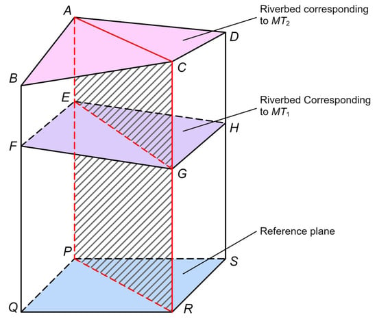
Figure 7.
The element for erosion and deposition calculations.

Table 1.
Coordinates of the vertices on the calculation element.
3. Results
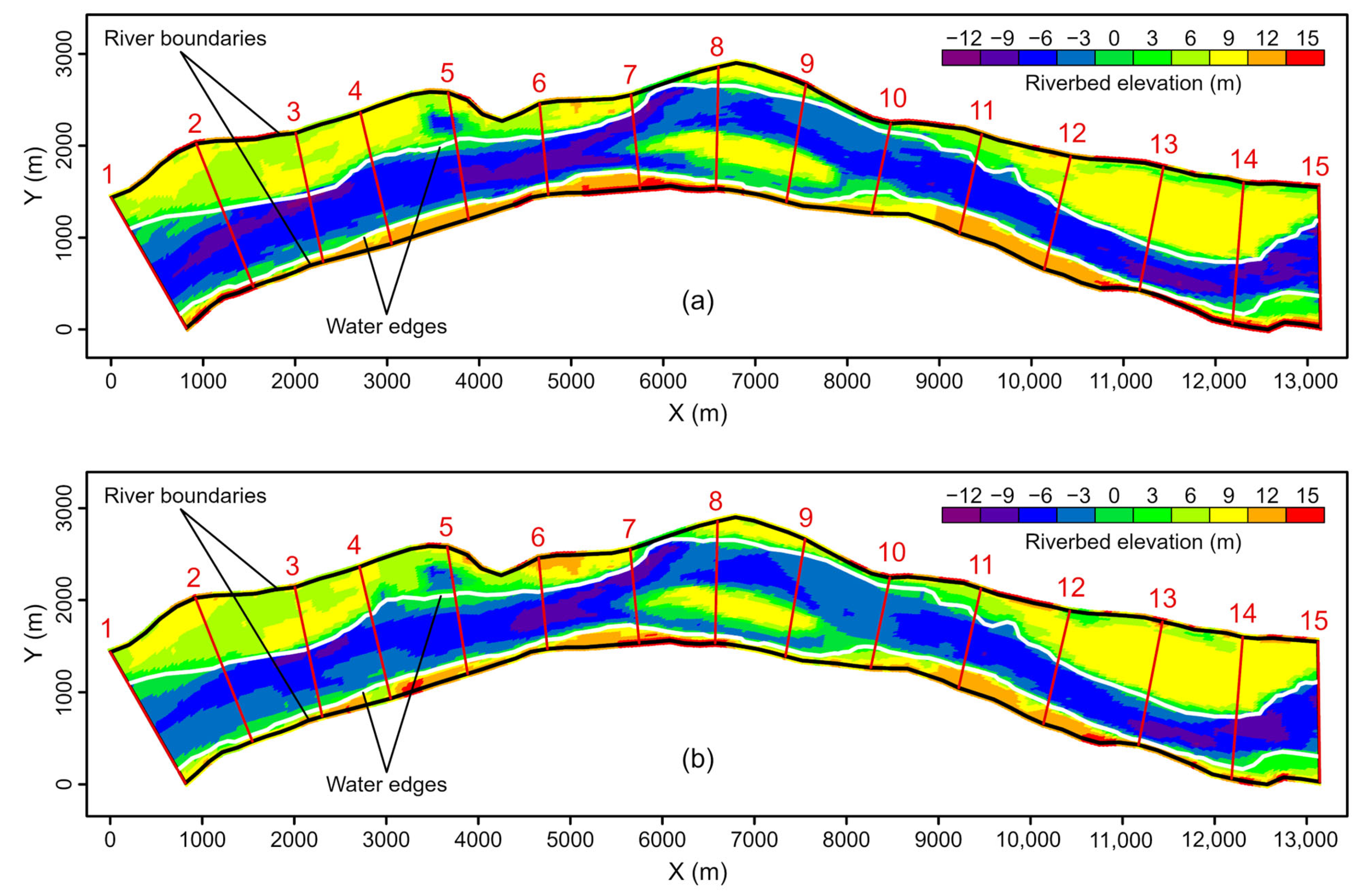
To validate the rationality and computational accuracy of the proposed method, we selected a 13.8 km reach of the Pearl River in China for verification. The reason for choosing this particular reach is that we have measured bathymetric data for this reach at two different measurement times. Figure 8a,b, respectively, illustrate the measured bathymetric data for this reach on 26 January 2012 and 15 February 2020. Using an average distance between adjacent sections (ADAS) of approximately 1.0 km, we extracted 15 cross-sections from each of these two datasets. These can be considered the measured cross-sectional terrain data corresponding to the two measurement times. These two sets of cross-sections will be used to calculate the erosion and deposition changes in this reach from 26 January 2012 to 15 February 2020. Figure 8a,b also include the riverway boundaries and water edges corresponding to the measurement times of the bathymetric data. Based on the extracted cross-sectional terrain data, the results obtained using the proposed method will be compared with the measured erosion and deposition changes, thereby verifying the rationality and computational accuracy of the method.
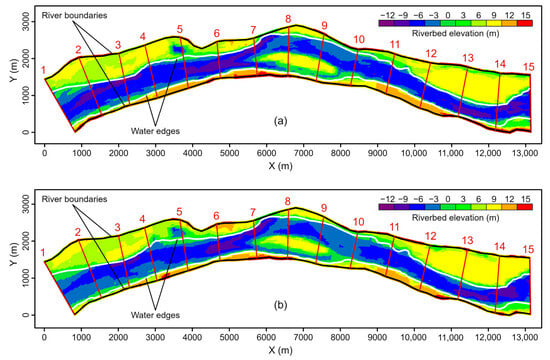
Figure 8.
Measured bathymetric data. (a) Measured in January 2012; (b) Measured in February 2020.
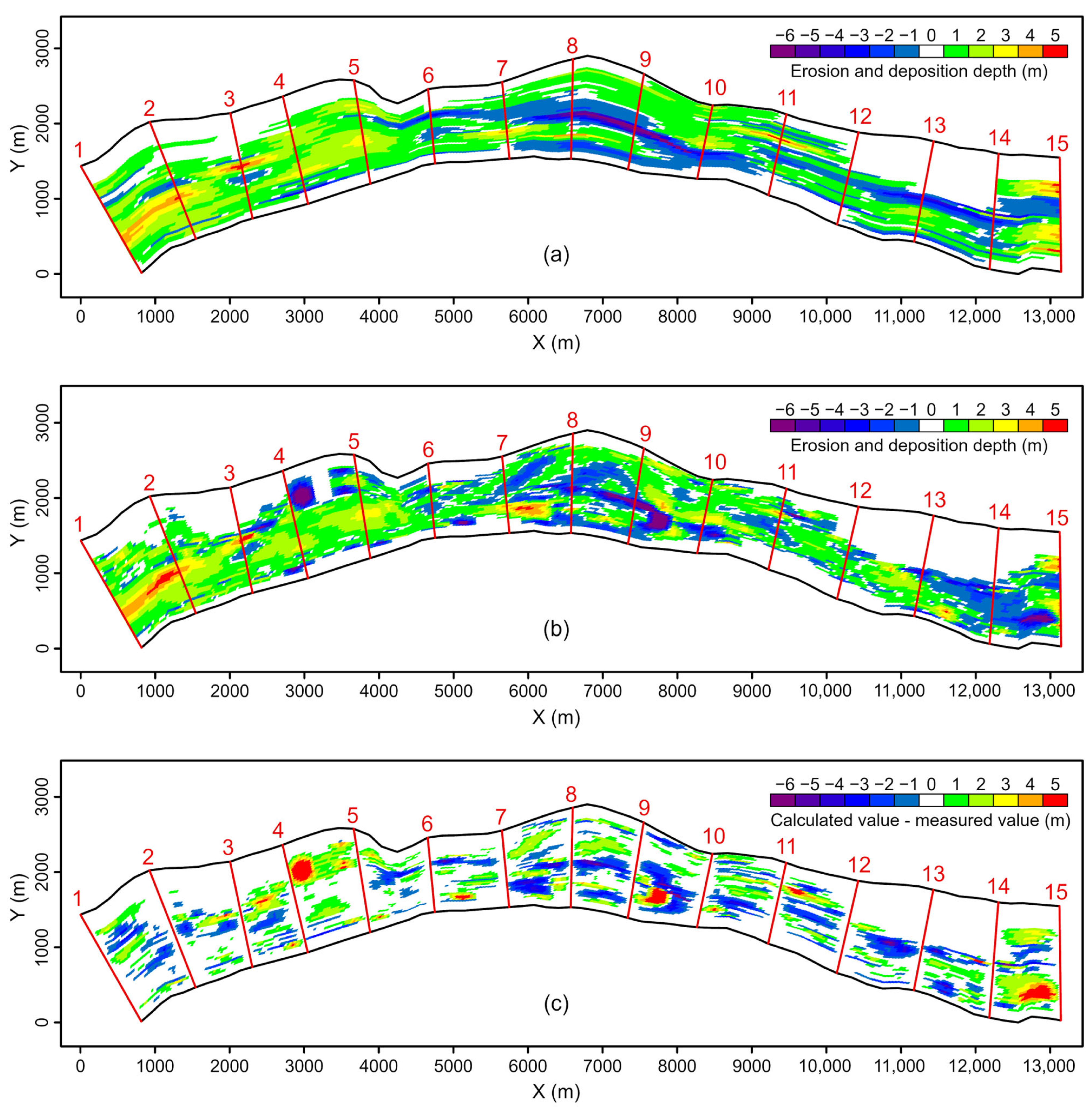
Figure 9 presents a comparison between the calculated values and the measured values of erosion and deposition changes in the riverway during the specified period. In Figure 9, it can be observed that the calculated values generally align well with the measured values for overall erosion and deposition changes in the reach. The calculated total volume of erosion and deposition for this reach is 2.625 × 10⁶ m3, while the measured value is 2.485 × 10⁶ m3, resulting in a relative error of only 5.6%. For specific segments of the reach, between cross-sections 1 to 5 and 10 to 15 (in relatively straight sections), the agreement between calculated and measured values is higher. The regions of erosion and deposition changes are consistent. However, between cross-sections 4 and 5, there is a significant area with erosion and deposition changes in the measured values (Figure 9b) that does not appear in the distribution map obtained using the proposed method (Figure 9a). This discrepancy is attributed to the fact that, in the method proposed in this paper, the riverbed terrain is interpolated based on the terrain data of adjacent cross-sections. Our interpolated terrain is always controlled by the elevation of the measured cross-sections. Natural riverway changes in bed erosion and deposition are influenced by both water and sediment conditions and bed boundary conditions. Cross-sections cannot sample every specific shape of the riverbed, leading to the neglect of some terrain changes between cross-sections. This can also be observed in Figure 9c, where the differences between the measured values and calculated values primarily occur in the region between two adjacent cross-sections. In the vicinity of the cross-sections, such differences are minimal. In the segment between cross-sections 5 and 10 (with a river center continent), the calculated and measured volume of the erosion and deposition are 0.016 × 10⁶ m3 and 0.035 × 10⁶ m3, respectively. However, due to the presence of a river center continent in this reach, the meandering morphology of the riverway is more complex. The spatial distribution of erosion and deposition changes obtained by the interpolation calculation differs somewhat from that calculated from measured values. Figure 10 provides a comparison between the calculated and measured volumes of erosion and deposition between adjacent cross-sections. To evaluate the average level of proximity between the calculated values and measured values for the erosion and deposition volume in various river segments, the Nash efficiency coefficient (NSE) was calculated, yielding a value of 0.88. This indicates that the proposed method in this paper exhibits good computational quality. Overall, the trend of changes is generally consistent, but there are occasional significant differences between certain pairs of adjacent cross-sections, such as between cross-sections 4 and 5, where interpolation fails to capture a significant area of erosion and deposition changes, resulting in a calculated value that is greater than the measured value.
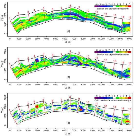
Figure 9.
Comparison of calculated and measured values of erosion and deposition changes in spatial distribution. (a) Calculated value; (b) Measured value; (c) Difference between calculated and measured value.
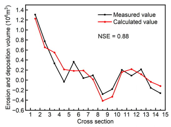
Figure 10.
Comparison of calculated and measured values of erosion and deposition volume between adjacent cross-sections.
4. Discussion
4.1. Comparison with the Cross-Section Method
We also employed the cross-section method proposed by Yang et al. [16] to calculate the erosion and deposition changes in the reach mentioned in Section 3, obtaining the total erosion and deposition volume for the entire reach (Table 2). In terms of the total erosion and deposition volume in the reach, the cross-section method calculated a value of 2.961 × 10⁶ m3, while the proposed method in this paper calculated a value of 2.625 × 10⁶ m3. These values represent a 19.2% and 5.6% overestimation, respectively, compared to the measured value of 2.485 × 10⁶ m3. This indicates that the proposed method in this paper exhibits a significant improvement in computational accuracy compared to the cross-section method. Figure 11 provides a comparison of erosion and deposition volume between adjacent cross-sections using different calculation methods. In Figure 11, it can be observed that the NSE for the proposed method in this paper is 0.88, while the NSE for the cross-section method is 0.71. This suggests that the proposed calculation method in this paper is superior to the cross-section method, with a higher level of agreement between the calculated values of erosion and deposition volume between adjacent cross-sections and the measured values. In relatively straight river sections, both the proposed method in this paper and the cross-section method yield similar results that align well with the measured values. However, in river sections with significant changes in the meandering morphology, the results obtained by the proposed method in this paper are closer to the measured values compared to the results from the cross-section method. This is because the cross-section method calculates erosion and deposition changes by approximating the river segment between two cross-sections as a truncated cone, relying heavily on the representative nature of the cross-sections and neglecting variations in width along the reach and the curvature of the river channel. In contrast, the method proposed in this paper divides the entire reach into grids, with the grid orientation controlled by auxiliary lines such as the riverway boundaries, fully considering changes in the channel width and channel curvature along the reach. In this respect, it is superior to the cross-section method.

Table 2.
Total erosion and deposition volume using the proposed method and the cross-section method.
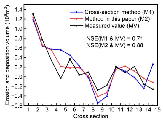
Figure 11.
Erosion and deposition volume between adjacent cross-sections using the proposed method and the cross-section method.
4.2. Grid Size Sensitivity Analysis
In a grid-based numerical method, the grid size can sometimes affect the accuracy of the results. In order to understand the influence of grid size on the calculation results in the proposed method, seven different grid sizes were set, and their corresponding calculation results were compared to analyze the grid size sensitivity. In the case study in Section 3 of this paper, the measured average spacing of the cross-sectional terrain data is 10.0 m. Based on this, grids with average sizes of 80.0 m, 40.0 m, 20.0 m, 10.0 m, 5.0 m, 3.0 m and 1.0 m were generated, and their corresponding erosion and deposition volumes were calculated (Table 3). It can be observed that as the grid size decreases, the error between the calculated values and the measured values decreases. However, when the grid size is less than 10.0 m, a further reduction in grid size does not result in significant changes in the outcomes. This is because, in the calculation of erosion and deposition according to the proposed method in this paper, all results are derived from cross-sectional terrain data. When the grid size is larger than the distance between adjacent measurement points on the cross-section, there is a certain degree of generalization of the cross-sectional terrain data, leading to a decrease in data resolution and introducing errors into the calculation results. When the grid size is smaller than this distance, a limited number of data points on the cross-section are still used as source data, but better results are not achieved. Thus, when using this method, the optimal grid size should be consistent with the measured average spacing of cross-sectional terrain data.

Table 3.
Total erosion and deposition volume with different grid sizes.
4.3. Impact of the Distance between Adjacent Cross-Sections on Calculation Accuracy
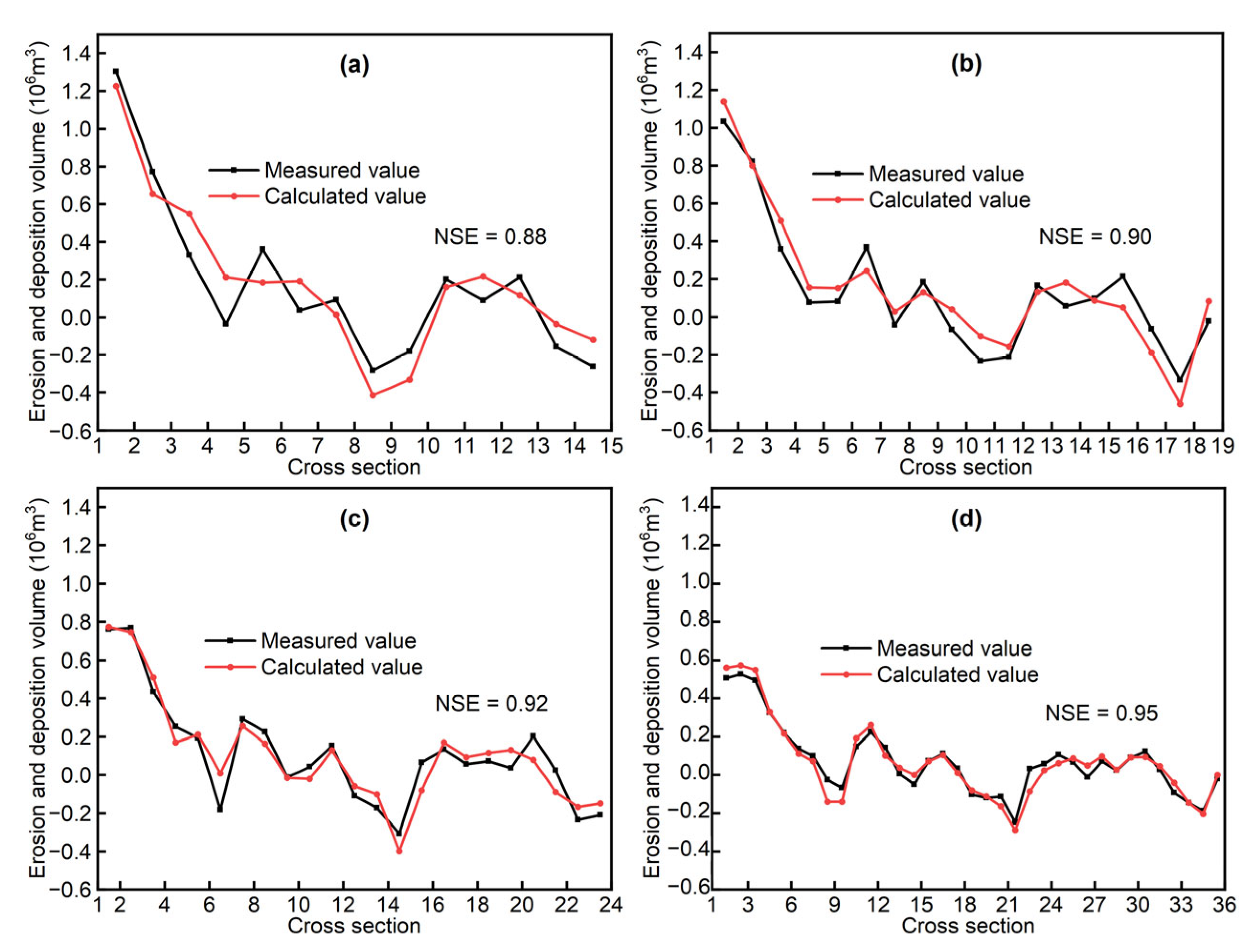
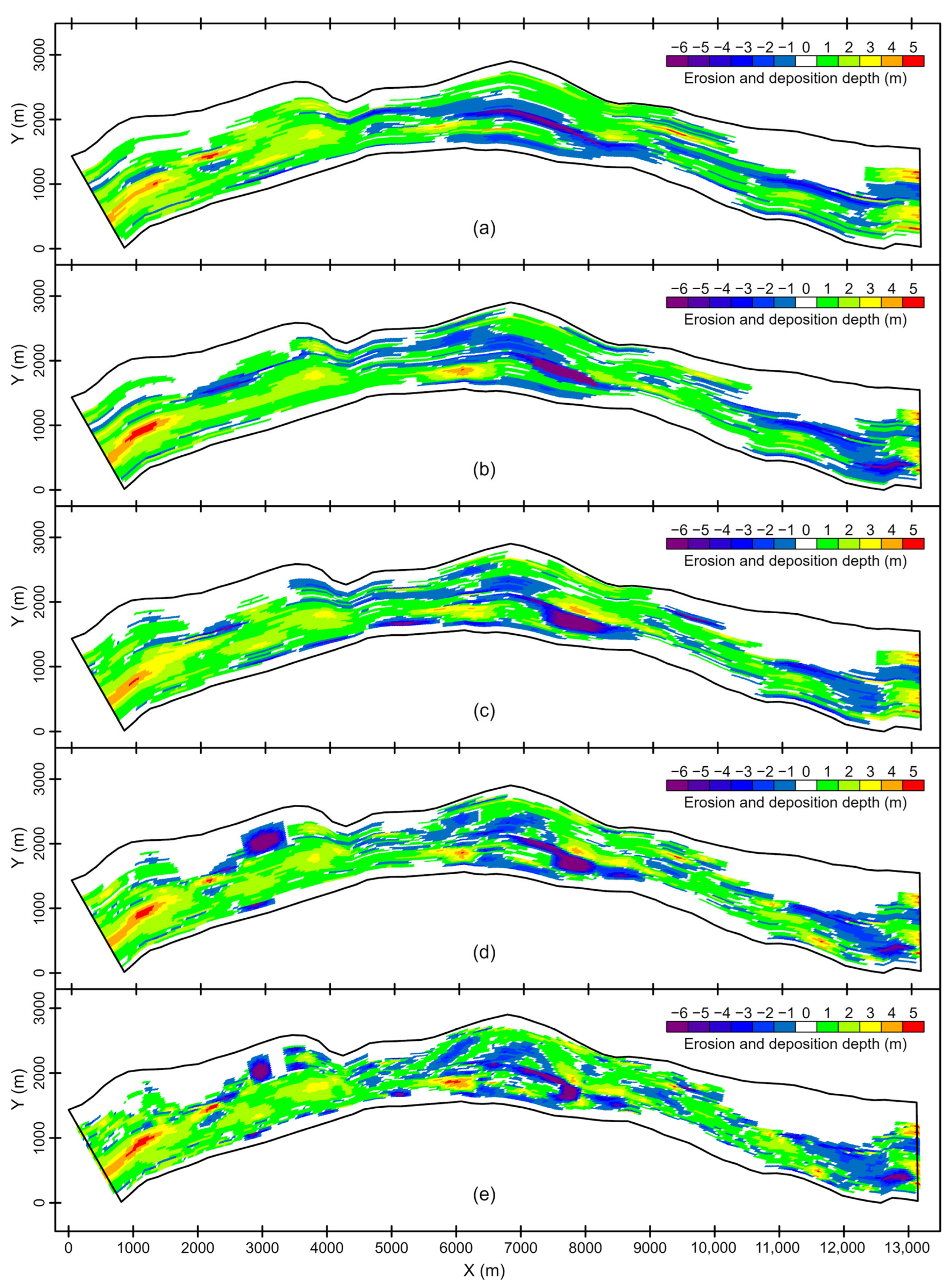
The distance between adjacent cross-sections is one of the crucial factors influencing the calculation accuracy. To compare the effect of ADAS on the accuracy of the proposed calculation method in this paper, the ADAS used in Section 3 was successively reduced from 1.0 km to 0.8 km, 0.6 km and 0.4 km. Correspondingly, the number of cross-sections increased from 15 to 19, 24 and 36, respectively. Table 4 provides the calculated erosion and deposition volume for the reach using different ADAS. It can be observed that as the ADAS decreases (i.e., the number of cross-sections increases), the calculated changes in erosion and deposition volume gradually approach the measured values. When the ADAS is 1.0 km, 0.8 km, 0.6 km and 0.4 km, the calculated changes in reach erosion and deposition are 2.625 × 10⁶ m3, 2.605 × 10⁶ m3, 2.397 × 10⁶ m3 and 2.423 × 10⁶ m3, respectively. These represent deviations of 5.6%, 4.8%, −3.5% and −2.5% from the measured value of 2.485 × 10⁶ m3. Figure 12 presents a comparison between the calculated and measured values of erosion and deposition volume between adjacent cross-sections for different ADASs. It is evident that as the ADAS decreases, the degree of agreement between the calculated values and the measured values increases. The ADAS decreases from 1.0 km to 0.8 km, 0.6 km and 0.4 km, resulting in an increase in the NES from 0.88 to 0.90, 0.92 and 0.95, respectively. Figure 13 illustrates the erosion and deposition distribution obtained using different ADASs. It can be observed that as the ADAS decreases, the degree of agreement between the calculated values and the measured values of erosion and deposition distribution continually improves. This allows for a more detailed representation of changes in erosion and deposition.

Table 4.
Total erosion and deposition volume with different ADASs.
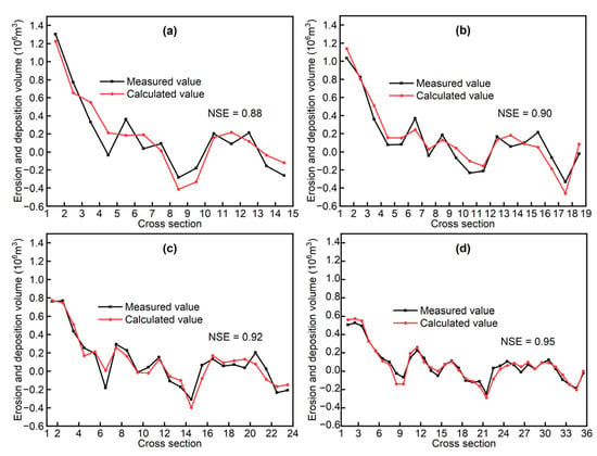
Figure 12.
Comparison of calculated and measured values of erosion and deposition volume between adjacent cross-sections using different ADASs. (a) 15 cross sections (ADAS = 1.0 km); (b) 19 cross sections (ADAS = 0.8 km); (c) 24 cross sections (ADAS = 0.6 km); (d) 36 cross sections (ADAS = 0.4 km).
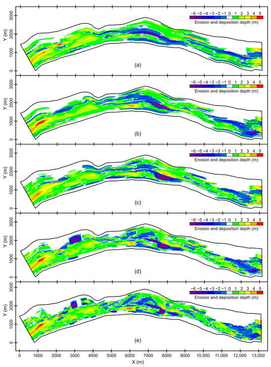
Figure 13.
Comparison of calculated and measured values of erosion and deposition changes in spatial distribution using different ADASs. (a) 15 cross sections (ADAS = 1.0 km); (b) 19 cross sections (ADAS = 0.8 km); (c) 24 cross sections (ADAS = 0.6 km); (d) 36 cross sections (ADAS = 0.4 km); (e) Measured value.
Therefore, it can be concluded that when calculating riverway erosion and deposition using the proposed method in this paper, the results are already superior to those obtained through the cross-section method when ADAS = 1.0 km. The results obtained with smaller ADASs are even closer to the measured values. In practical applications of this method, an appropriate ADAS should be chosen based on the characteristics of the river and the computational distance. With the development of river digital twinning and smart water management, more accurate data on river erosion and deposition changes are needed as support. When economic, human and time costs permit, using high-resolution river bathymetric data to reflect changes in riverway erosion and deposition is a preferable choice. However, if only cross-sectional terrain data are available, the method proposed in this paper remains a good approach to obtaining accurate erosion and deposition changes and their spatial distribution.
5. Conclusions
In this paper, a method for calculating riverway erosion and deposition using measured cross-sections is proposed, and detailed calculation steps are provided. The method generates a quadrilateral grid in the calculation domain by introducing auxiliary lines, such as riverway boundaries and water edges. It not only calculates accurate erosion and deposition changes but also provides their spatial distribution.
The proposed method was validated using measured data. The results show that the relative error between the calculated and measured values of the total erosion and deposition volume is only 5.6%. A comparison with the results of the cross-section method reveals that, at a cross-section spacing of 1.0 km, the overall accuracy of the proposed method is better than that of the cross-section method. The impact of the cross-section spacing on the results of the proposed method is discussed, showing that as the distance between adjacent cross-sections decreases from 1.0 km to 0.4 km, the relative error between the calculated and measured values of total erosion and deposition volume decreases from 5.6% to 2.5%.
When faced with the need to calculate changes in riverway erosion and deposition, the proposed method based on measured cross-sections can provide accurate data on erosion and deposition changes and their spatial distribution.
Author Contributions
X.Z., project administration; funding acquisition; and writing—review and editing. Z.B., methodology; software, writing—original draft; and writing—review and editing. J.L., conceptualization; supervision; validation; methodology; and writing—review and editing. Z.X., investigation; data curation; and writing—review and editing. X.G., investigation; data curation; and writing—review and editing. All authors have read and agreed to the published version of the manuscript.
Funding
This work was supported by the National Natural Science Foundation of China (Grant Nos. U2243220, 41930643, 52079053); the Research Fund of Key Laboratory of Water Management and Water Security for Yellow River Basin, Ministry of Water Resources (under construction) (Grant No. 2022-SYSJJ-10); and the project Study on Dawen River Flood Forecast and Dongping Lake (Old Lake) Operation Mode.
Data Availability Statement
Some or all of the data and 1137 lines of Fortran codes and 326 lines of Python codes used in this study are available from the corresponding author upon reasonable request.
Conflicts of Interest
The authors declare no conflict of interest.
References
- Angelakis, A.N.; Capodaglio, A.G.; Valipour, M.; Krasilnikoff, J.; Ahmed, A.T.; Mandi, L.; Tzanakakis, V.A.; Baba, A.; Kumar, R.; Zheng, X.; et al. Evolution of Floods: From Ancient Times to the Present Times (ca 7600 BC to the Present) and the Future. Land 2023, 12, 1211. [Google Scholar] [CrossRef]
- Yin, Z.; Zhang, H.; Tan, G.; Lyu, Y.; Feng, Z.; Shu, C.; Wang, J.; Zhang, G. Operating Effects of the Three Gorges Reservoir on the Riverbed Stability in the Wuhan Reach of the Yangtze River. Water 2021, 13, 3353. [Google Scholar] [CrossRef]
- Yang, Z.; Duan, X.; Huang, J.; Dong, Y.; Zhang, X.; Liu, J.; Yang, C. Tracking long-term cascade check dam siltation: Implications for debris flow control and landslide stability. Landslides 2021, 18, 3923–3935. [Google Scholar] [CrossRef]
- Han, D.; He, Z.; Lin, Y.T.; Wang, Y.; Guo, Y.; Yuan, Y. Hydrodynamics and sediment transport of downslope turbidity current through rigid vegetation. Water Resour. Res. 2023, 59, e2023WR034421. [Google Scholar] [CrossRef]
- Zhou, M.; Xia, J.; Deng, S.; Shen, J.; Mao, Y. Modelling of phosphorus and nonuniform sediment transport in the Middle Yangtze River with the effects of channel erosion, tributary confluence and anthropogenic emission. Water Res. 2023, 243, 120304. [Google Scholar] [CrossRef] [PubMed]
- Azarang, F.; Telvari, A.; Sedghi, H.; Bajestan, M.S. Numerical simulation of flow and sediment transport of Karkheh river before the reservoir dam construction using MIKE 11 [a case study in Iran]. Adv. Environ. Biol. 2014, 8, 979–989. [Google Scholar]
- Adib, A.; Foladfar, H.; Argashi, N. Application of Fluvial-12 model for calculation of maximum deformation in cross sections of tidal rivers (the Karun River in Iran). Acta Sci. Technol. 2019, 41, e39539. [Google Scholar] [CrossRef]
- Shu, C.; Tan, G. Advances in calculation methods for river sedimentation. J. Sediment. Res. 2009, 68–73. (In Chinese) [Google Scholar] [CrossRef]
- Dong, Y.H. Contrast study on Estimation of River Deposition Erosion Amount by Sediment Budget Method and Morphological Change Method. J. Yangtze River Sci. Res. Inst. 2009, 26, 1. (In Chinese) [Google Scholar]
- Duan, G.; Peng, Y.; Guo, M. Comparative analysis on riverbed erosion and deposition amount calculated by different methods. J. Yangtze River Sci. Res. Inst. 2014, 31, 108. (In Chinese) [Google Scholar]
- Zhang, R.; Wang, Y.; Han, Q.; Wu, B.-S. Calculation methods for erosion and deposition based on sediment balance equation in the Lower Yellow River. J. Sediment Res. 2018, 43, 21–27. (In Chinese) [Google Scholar]
- Antoine, G.; Camenen, B.; Jodeau, M.; Némery, J.; Esteves, M. Downstream erosion and deposition dynamics of fine suspended sediments due to dam flushing. J. Hydrol. 2020, 585, 124763. [Google Scholar] [CrossRef]
- Guo, Q.; Zheng, Z.; Huang, L.; Deng, A. Regularity of sediment transport and sedimentation during floods in the lower Yellow River, China. Int. J. Sediment Res. 2020, 35, 97–104. [Google Scholar] [CrossRef]
- Zhang, S.; Hu, X.; Miao, W.; Xu, Z. Analysis of the sediment sources of flood driven erosion and deposition in the river channel of the Fu River Basin. Int. J. Sediment Res. 2023, 38, 653–661. [Google Scholar] [CrossRef]
- Yang, Y.; Zhang, M.; Zhu, L.; Zhang, H.; Liu, W.; Wang, J. Impact of the operation of a large-scale reservoir on downstream river channel geomorphic adjustments: A case study of the Three Gorges. River Res. Appl. 2018, 34, 1315–1327. [Google Scholar] [CrossRef]
- Yang, Y.; Zheng, J.; Zhang, M.; Zhu, L.; Zhu, Y.; Wang, J.; Zhao, W. Sandy riverbed shoal under anthropogenic activities: The sandy reach of the Yangtze River, China. J. Hydrol. 2021, 603, 126861. [Google Scholar] [CrossRef]
- Liu, X.; Shi, C.; Zhou, Y.; Gu, Z.; Li, H. Response of Erosion and Deposition of Channel Bed, Banks and Floodplains to Water and Sediment Changes in the Lower Yellow River, China. Water 2019, 11, 357. [Google Scholar] [CrossRef]
- Xia, J.; Deng, S.; Zhou, M.; Lu, J.; Xu, Q. Geomorphic response of the Jingjiang Reach to the Three Gorges Project operation. Earth Surf. Process. Landf. 2017, 42, 866–876. [Google Scholar] [CrossRef]
- Yuan, X.; Tian, F.; Wang, X.; Liu, Y.; Chen, M.T. Small-scale sediment scouring and siltation laws in the evolution trends of fluvial facies in the Ningxia Plain Reaches of the Yellow River (NPRYR). Quat. Int. 2018, 476, 14–25. [Google Scholar] [CrossRef]
- Lyu, Y.; Zheng, S.; Tan, G.; Shu, C.; Han, Q. Morphodynamic adjustments in the Yichang–Chenglingji Reach of the Middle Yangtze River since the operation of the Three Gorges Project. Catena 2019, 172, 274–284. [Google Scholar] [CrossRef]
- Liu, W.; Wang, S.; Sang, Y.F.; Ran, L.; Ma, Y. Effects of large upstream reservoir operations on cross-sectional changes in the channel of the lower Yellow River reach. Geomorphology 2021, 387, 107768. [Google Scholar] [CrossRef]
- de Sousa, L.S.; Raude, J.M.; Wambua, R.M.; Mutua, B.M. Bathymetry changes caused by sedimentation in an unlined canal of the Chókwè irrigation scheme, Mozambique. Irrig. Drain. 2022, 71, 783–803. [Google Scholar] [CrossRef]
- Xu, H.; Xia, Y.F.; Wen, Y.C. Study on Characteristics of River Evolution of Chengtong Reach in the Lower Reach of the Yangtze River before and after Operation of the Three Gorges Project. In APAC 2019, Proceedings of the 10th International Conference on Asian and Pacific Coasts 2019, Hanoi, Vietnam, 25–28 September 2019; Springer: Singapore, 2020; pp. 745–749. [Google Scholar]
- Kou, Y.; Wang, N.; An’an Chen, K.L. Monitoring Variation of Glaciers Based on Remote Sensing Images in the Chenab Basin, Western-Himalaya, 1993~2016. Remote Sens. Technol. Appl. 2020, 35, 712–722. [Google Scholar]
- Schepaschenko, D.; See, L.; Lesiv, M.; Bastin, J.F.; Mollicone, D.; Tsendbazar, N.E.; Bastin, L.; McCallum, I.; Bayas, J.C.L.; Baklanov, A.; et al. Recent advances in forest observation with visual interpretation of very high-resolution imagery. Surv. Geophys. 2019, 40, 839–862. [Google Scholar] [CrossRef]
- Zhao, B.; Liu, Y.; Wang, L. Evaluation of the Stability of Muddy Coastline Based on Satellite Imagery: A Case Study in the Central Coasts of Jiangsu, China. Remote Sens. 2023, 15, 3323. [Google Scholar] [CrossRef]
- Xia, M.; Cui, Y.; Zhang, Y.; Xu, Y.; Liu, J.; Xu, Y. DAU-Net: A novel water areas segmentation structure for remote sensing image. Int. J. Remote Sens. 2021, 42, 2594–2621. [Google Scholar] [CrossRef]
- Pan, Y.; Xia, J.; Yang, K. A method for digital terrain reconstruction using longitudinal control lines and sparse measured cross sections. Remote Sens. 2022, 14, 1841. [Google Scholar] [CrossRef]
Disclaimer/Publisher’s Note: The statements, opinions and data contained in all publications are solely those of the individual author(s) and contributor(s) and not of MDPI and/or the editor(s). MDPI and/or the editor(s) disclaim responsibility for any injury to people or property resulting from any ideas, methods, instructions or products referred to in the content. |
© 2023 by the authors. Licensee MDPI, Basel, Switzerland. This article is an open access article distributed under the terms and conditions of the Creative Commons Attribution (CC BY) license (https://creativecommons.org/licenses/by/4.0/).

