Abstract
In the wake of the terrorist attacks of 11 September 2001, extensive research efforts have been dedicated to the development of computational algorithms for identifying contamination sources in water distribution systems (WDSs). Previous studies have extensively relied on evolutionary optimization techniques, which require the simulation of numerous contamination scenarios in order to solve the inverse-modeling contamination source identification (CSI) problem. This study presents a novel framework for CSI in WDSs using Bayesian optimization (BO) techniques. By constructing an explicit acquisition function to balance exploration with exploitation, BO requires only a few evaluations of the objective function to converge to near-optimal solutions, enabling CSI in real-time. The presented framework couples BO with EPANET to reveal the most likely contaminant injection/intrusion scenarios by minimizing the error between simulated and measured concentrations at a given number of water quality monitoring locations. The framework was tested on two benchmark WDSs under different contamination injection scenarios, and the algorithm successfully revealed the characteristics of the contamination source(s), i.e., the location, pattern, and concentration, for all scenarios. A sensitivity analysis was conducted to evaluate the performance of the framework using various BO techniques, including two different surrogate models, Gaussian Processes (GPs) and Random Forest (RF), and three different acquisition functions, namely expected improvement (EI), probability of improvement (PI), and upper confident bound (UCB). The results revealed that BO with the RF surrogate model and UCB acquisition function produced the most efficient and reliable CSI performance.
1. Background
Since the terrorist attacks on 11 September 2001, there has been a heightened focus on securing water infrastructure. One crucial aspect that has received significant attention in recent years is the development of methods and algorithms for rapidly detecting water contaminants that may enter into drinking water distribution systems (WDSs). Contaminants entering the WDS through either accidental intrusion or intentional injection may spread rapidly and unpredictably through the pipes of the WDS. As a result, rapid identification of contamination events is essential for managing water quality and protecting public health and safety. By employing sophisticated algorithms and advanced sensing technologies, water utilities can promptly identify and respond to contamination incidents. This proactive approach plays a vital role in ensuring the security and safety of the water supply system, thereby safeguarding public health and well-being.
WDS pipes typically extend across vast distances, often spanning hundreds or even thousands of kilometers, with the majority of them buried underground [1]. This extensive pipe network makes it challenging to achieve ubiquitous monitoring of the entire system [2,3]. To enable an early warning and contamination response, numerous studies have focused on developing algorithms to optimize the placement of monitoring sensors [4]. These efforts aim to strategically position sensors throughout the network to maximize network coverage and contamination detection capabilities [5]. The latter was achieved by implementing different metrics, including minimizing the time to identify contamination events and minimizing the consumption of contaminated water [6,7,8,9]. Despite these extensive efforts, there is still a significant need for developing novel algorithms that can support early-warning systems by enabling real-time identification of contamination sources based on the monitoring data.
The contamination source identification (CSI) problem entails detecting the location, injection pattern, and injection concentration of a contamination source. Solving the inverse problem of identifying inputs (i.e., sources) from outputs (i.e., monitoring data) involves significant uncertainty due to the non-unique input–output relationship [10]. That is, different contamination sources could produce the same signal at the monitoring locations, making it challenging to accurately identify the true injection characteristics. This complexity can be further compounded by the occurrence of multiple contamination events simultaneously, the intricate topology of the water distribution network, and the inherent uncertainties in water quality monitoring data and simulation models, which makes predicting the correct pathway of the contaminant in the system very challenging [11].
2. Literature Review
Numerous research studies have attempted to design algorithms to identify contamination sources by utilizing observations from online monitoring stations. Early studies have generally attempted to frame the CSI problem as an inverse modeling problem. In study [12] an origin-tracking algorithm coupled with a nonlinear optimization technique to solve the inverse problem of identifying pollution sources’ injection time and location. The origin tracking model, employed to replace EPANET, reformulates the partial differential equations into a set of algebraic constraints. The latter describes the time delays between pipe boundary concentrations and connected nodes, removing the need for spatial discretization along the length of the pipes. Another study proposed a simulation–optimization approach in which EPANET was used to generate simulated concentrations at preselected monitoring locations, while the nonlinear reduced gradient method was employed to identify candidate contaminant sources by minimizing errors between simulated and observed concentrations at the monitoring locations [13]. A forward linear programming model trees—an extension of regression trees— was used to replace EPANET [14]. This was followed by formulating a linear programming framework that uses the model trees’ linear rule classification structure to solve the inverse problem and estimate the contamination injection sources’ time, location, and concentration. De Sanctis et al. [15] used a linear particle backtracking algorithm (PBA) to identify the water flow paths and travel times leading to each sensor reading. Accordingly, locations and times exhibiting positive sensor measurements but lacking negative ones were considered potential sources. A contamination status algorithm was then used to iteratively update the pollution possibility status for all candidate source locations and time intervals.
In addition to the aforementioned attempts, more recent efforts have generally focused on introducing evolutionary computation approaches, as well as probabilistic and machine learning algorithms, to solve the CSI problem [16]. A research by Liu et al. introduced an adaptive dynamic optimization technique that uses multiple population-based searches based on evolutionary algorithms (EAs) [17]. A distinct study developed a CSI model using a simulation–optimization approach in which EPANET was coupled with a MapReduce-based Parallel Niche Genetic Algorithm (GA) to generate contamination events based on the fitness values [18]. This study demonstrated that the simulation–optimization-based procedure has higher accuracy compared to the other approaches. Bayesian probabilistic approach, the beta-binomial conjugate pair structure, was utilized to identify contaminant source characteristics [11]. The algorithm allocated probabilities to potential source nodes based on false positive or negative data from monitoring stations, updating them using backtracking theory and Bayesian statistics. Overall, the proposed algorithm exhibited better responsiveness to sensor signal changes than a simple Bayes’ rule approach. A Random Forest machine learning algorithm was trained using numerous contamination scenarios (location, dosage, start time, and duration) that were generated through a Monte Carlo approach [19]. The study assessed the impact of sensor layout, imperfect sensor measurements, and demand uncertainty. The results demonstrated that the Random Forest algorithm achieved accurate predictions of the true pollution source, with increased accuracy corresponding to larger input datasets. However, the study was limited to the identification of a single injection scenario rather than multiple source scenarios. Different study compared three CSI techniques: Bayesian Probability-Based, Contaminant Status Algorithm, and mixed-integer linear programming (MILP) [20]. Their evaluation focused on accuracy and specificity metrics under various parameters, including WDS complexity, imperfect sensors, modeling error, number and timing of contaminant injections, and sensor coverage. Their results demonstrated that the optimization-based MILP method performed the best, particularly in scenarios with significant sensor noise. However, it requires tuning parameters that can impact real-world water network performance to achieve optimal solutions.
3. Study Contributions
Previous studies have largely focused on solving the CSI problem by utilizing a range of linear programming approaches, evolutionary optimization techniques, and statistical/machine learning methods. While linear approaches are recognized for their robustness and simplicity, their application has generally been limited to simple scenarios featuring only one contamination source. On the other hand, evolutionary optimization approaches require significantly higher computational time, as they typically involve conducting numerous evaluations of the objective function(s). The latter entails running a numerical simulation model (e.g., EPANET), where the partial differential equations governing the material transported in the WDS are numerically solved [21]. The high computational cost of evolutionary algorithms hinders the real-time identification of contamination sources. While machine learning algorithms overcome this limitation by shifting most of the computational burden to the training phase, they are greatly dependent on the quality of the training data, which are typically generated using numerical models (e.g., EPANET). Additionally, advanced data-driven models are inherently prone to overfitting. Thus, model errors could further propagate into CSI algorithms and compromise their outcomes.
In recent years, Bayesian optimization (BO) has gained considerable popularity due to its efficiency in the derivative-free optimization of black-box objective functions [22,23,24]. Instead of directly optimizing the computationally expensive objective function, BO builds a probabilistic model to estimate both the function’s output at unseen points, as well as a measure of uncertainty or confidence in those estimates. The core of BO lies in its ability to balance exploration (trying out new, uncertain points) and exploitation (focusing on areas known to contain good solutions). To decide where to sample next, an explicit acquisition function is derived from the model’s predictions incorporating both the predicted value and uncertainty. Thus, BO tends to require fewer function evaluations to find optima compared to other optimization approaches, earning it significant popularity for scenarios where evaluations are costly or time-consuming, such as hyperparameter tuning in machine learning models [25,26,27,28]. Other areas in which BO showed strong performance include materials design [29], robotics control [30], and drug discovery [31].
This study presents the first attempt at applying BO to solve the CSI problem in WDSs. This is accomplished by developing a simulation–optimization framework that combines EPANET with BO. The framework is implemented to conduct a sensitivity analysis of various BO techniques (including different covariance kernels and acquisition functions), coupled with an assessment of the role played by different BO parameters under diverse scenarios. Contrary to the majority of the previous CSI studies, which assumed a conservative (i.e., non-reactive) contaminant, the presented framework considers the contaminant to undergo reactions as it moves through the WDS. The significance of considering a reactive, rather than a conservative, contaminant is that reactions can further complicate the non-uniqueness challenge of CSI.
4. Methodology
4.1. Problem Formulation and CSI Framework
The presented simulation–optimization CSI framework involves coupling a water quality simulation model (EPANET) with an optimization algorithm (BO) to solve the CSI problem in WDSs. The CSI problem is defined herein as revealing the characteristics of multiple contamination sources given some sensory data. The objective function is formulated with the aim of minimizing the difference between the contaminant concentrations simulated using EPANET and those measured using sensors placed at specific locations within the network:
where and are the observed and simulated concentrations at sensor location i and time . A value close to zero indicates a higher likelihood of the simulated contamination event being the true contamination event. The decision variables in the optimization problem represent the characteristics of the simulated contamination event, namely the locations, start times, end times, and concentrations of the contamination sources.
Figure 1 shows a schematic of the closed-loop CSI framework developed in this study. First, the algorithm generates an initial set of random contamination events to build the prior of the BO probabilistic surrogate model. Each contamination event is characterized by different contaminant injection locations, durations, and concentrations. Second, the Water Network Tool for Resilience (WNTR) is used as a Python wrapper of EPANET to simulate WDS hydraulics and water quality [32]. That is, WNTR is used to simulate the contaminant concentrations at the designated sensor locations for each of the contamination events. Third, the probabilistic surrogate model, which predicts the simulated concentration and the associated uncertainty for a given contamination event, is updated with the results of the WNTR simulation. Fourth, the BO acquisition function is employed to evaluate the deviation between the observed and the simulated concentrations at the sensor locations, and propose the next point to sample (i.e., the next contamination event to simulate) to balance exploration and exploitation. As more contamination events are sampled, the probabilistic model is sequentially updated, producing more accurate estimates, which helps the algorithm converge to an optimal solution. After a given stoppage criterion (e.g., a predefined number of iterations with no significant improvement in the objective function), the algorithm is terminated, and the contamination event featuring the minimum deviation between simulated and observed concentrations is selected as the best solution. To execute the BO steps, the “pyGPGO” Python 3.8 package was used in this study, which allows the choice of different surrogate models, covariance functions, acquisition functions, and hyperparameters [33].
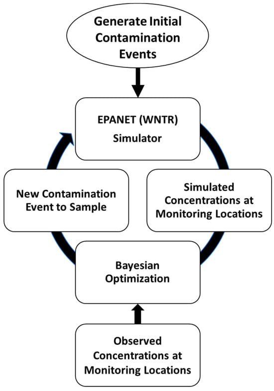
Figure 1.
BO framework for contamination source identification in WDSs.
4.2. Bayesian Optimization
BO is comprised of two key components: the surrogate function and the acquisition function. The former constitutes a method for predicting the value of the objective function at any point together with an estimate of the uncertainty in this prediction, while the latter is a method for deciding where to sample based on the posterior probability distribution obtained from the surrogate model [23].
4.2.1. Probabilistic Surrogate Model
In this study, we investigated two of the most widely adopted approaches to fit the surrogate model within the context of BO, namely Gaussian Process (GP) regression and Random Forest (RF) regression [34]. Both models constitute non-parametric, probabilistic approaches that can model complex nonlinear relationships.
Gaussian Process Regression
A GP is a collection of random variables, any finite number that has a joint Gaussian distribution. In GP regression, it is used to define a prior over functions. Each function in this space is characterized by a mean function, ), and a covariance kernel, [35]:
The choice of kernel function is crucial in GP regression as it defines the covariance between any two points in the input space, determining how the similarity between inputs influences the regression output. In this study, four of the commonly used kernel functions for GP regression were tested for the problem of CSI in WDSs, namely squared-exponential, Matérn 3/2, rational quadratic, and gamma-exponential [22].
As highlighted by Melkumyan and Nettleton [36], the squared-exponential (SE) function is the most commonly used choice for the covariance (kernel) function, and can be represented as
where is the Euclidean distance between and , , and is the characteristic length scale of the covariance kernel.
The gamma-exponential (GE) kernel is a modified version of the SE kernel, which is controlled by a hyperparameter () that further adjusts the smoothness of the kernel:
The Matérn 3/2 (M32) kernel function is considered a general case of the SE kernel:
The rational quadratic (RQ) kernel can be specified as follows:
where is a positive-valued scale-mixture parameter.
It is noteworthy that when the covariance between and is close to one, this indicates a belief that and are likely to be very similar, and they have substantial mutual influence. Conversely, a covariance close to zero indicates that and are unrelated and have negligible impact on one another [29]. This concept is fundamental to converging the search space and achieving the best sequential sampling pathway.
Random Forest Regression
RF is a popular supervised machine learning technique used to solve classification and regression problems. RF is an ensemble learning method; that is, it combines the predictions from multiple machine learning algorithms to make more accurate predictions than any individual model. It operates by constructing a multitude of decision trees at training time and outputting the mean prediction of the individual trees for regression problems, or the mode of the classes (i.e., the most common output class) for classification problems [37]. Each of the decision trees in an RF is trained on a random subset of the training data, and a random subset of the input features is used. This approach is known as “bootstrap aggregating” or “bagging”, which helps reduce the variance of the RF model, making it less likely to overfit the training data [38].
Assume T represents the number of decision trees, and Mi(x) is the output of the i-th decision tree for the input x. An average of T (i.e., decision variables) has a variance, , where σ2 is a variance of each decision tree. The variance of the average could be computed as follows [35]:
where is the positive pairwise correlation of the identically distributed variables [38]. Accordingly, we may deduce that the correlation between the variance of the RF estimator and and σ2 is positive but not with the size of the forest (T).
4.2.2. Acquisition Function
The acquisition function is the second primary component of the BO framework. Its role is to determine where to sample the next area of the posterior distribution that is derived from the surrogate model. The main task of the acquisition function is to guide the search to locations that have potential improvement toward finding the optimal solution of the objective function . It achieves this by selecting a point where either the predicted value for the objective function is promising (exploitation), the uncertainty of that prediction is high (exploration), or a combination of both [22]. Accordingly, to balance exploration and exploitation, the acquisition function evaluates the trade-off between exploring uncertain regions of the posterior distribution and exploiting promising points in the multivariate distribution of the objective function. In this study, we consider three commonly used types of acquisition functions:
Probability of Improvement
The probability of improvement (POI) can be written as
The equation above selects the next sampling location as the one that has the highest probability of improving over the current best estimate of the objective function () observed so far. Here, and are the mean and standard deviation of the posterior constructed using the surrogate model, and indicates the normal CDF.
POI favors points with a high probability of being greater than . The latter indicates that POI is biased toward exploitation [39]. Therefore, a new term ϵ is introduced to the formula above in order to regulate the balance between exploration and exploitation. A high value of ϵ guides the next query sampling point toward exploration, while indicates pure exploitation.
Expected Improvement
Expected improvement (EI) is the most widely used acquisition function with BO [40]. EI calculates the improvement expectation on the objective function with respect to the predictive distribution of the surrogate model. EI selects the point to sample next as the one that has the greatest expected improvement over the current best value of the objective function observed so far.
EI can be mathematically expressed as follows [35]:
where represents the CDF, is the pdf, and is a term added to the expression to manage and moderate the trade-off between exploration and exploitation.
Upper Confidence Bound
The Upper Confidence Bound (UCB) acquisition function depends on the Confidence-Bound theory to choose the next point for objective function evaluation [41,42]. The UCB function is defined as the weighted sum of the predicted mean and the standard deviation of the objective function:
Based on the above equation, it can be seen that UCB offers a straightforward approach to balance exploitation and exploration since , the term introduced to the equation, directly controls the trade-off between exploration and exploitation. For a small value of , BO will search for the areas that have promising performance (i.e., high ), while a large will guide the search space toward uncertain areas (exploration).
4.3. Case Study
The presented framework was applied to two case study WDSs with varying degrees of complexity to demonstrate the performance of BO for CSI under various conditions. The first case study features a well-known medium-sized network, EPANET Net3, which comprises 92 nodes, 2 water sources, 3 elevated storage tanks, 2 pumps, and 117 pipes (Figure 2). The second case study features a real-world, large-scale WDS, known as the Richmond network, which comprises 865 junctions, 1 reservoir, 6 elevated storage tanks, and 949 pipes (Figure 3). The Richmond Water Network model was obtained from the study by Grbčić et al. [19]. Monitoring nodes were strategically positioned in both WDSs based on previous literature. In the case of Net3, the sensor layout was obtained from the study by Seth et al. [20]. The authors employed TEVA-SPOT, integrated into EPA’s Water Security Toolkit, to optimize the sensor placement. The results found the optimal locations for the sensors to be at nodes 117, 149, 167, 213, and 253 (Figure 2). Similarly, for the Richmond network, the monitoring network layout was obtained from the studies by Grbčić et al. [19] and Preis and Ostfeld [43]. The sensors in this network were optimally placed at nodes 93, 352, 428, 600, and 672 (see Figure 3).
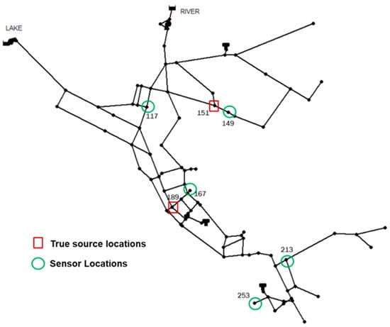
Figure 2.
Net3 layout.
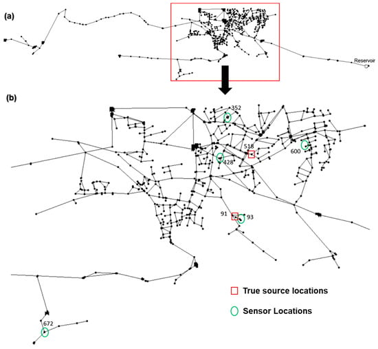
Figure 3.
Richmond Water Network layout. (a) the whole Richmond Water Network. (b) Richmond Water Network detailed with sensor and source locations.
The hydraulics of the two water networks were simulated hourly over a 24 h duration for the Net3 network, and 48 h for the Richmond network. Contaminant injection was simulated at a 5 min interval, and the contaminant concentration values at the sensors were monitored at the end of each 5 min timestep. Table 1 lists hydraulic and network parameters for both WDSs. It is worth noting that, as Seth et al. [20] indicated, short-duration contaminant injections significantly influence the identification of contamination source characteristics, particularly when the injection period is less than 4 h. Consequently, all contaminant source patterns considered in this study have a duration of 2 h.

Table 1.
Simulation Parameters for the Case Study Networks.
Three different contaminant injection patterns were investigated in this study as illustrated in Figure 4 and represented in Table 2. Pattern 1 forms a continuous, time-dependent intrusion (uniform pattern injection) initiated at 2 a.m. and lasting until 4 a.m. On the other hand, Pattern 2 was designed to be more complicated than Pattern 1, exhibiting a doubling in the concentration of contaminants after 1 h. Pattern 3, the most complex of the three, combines Patterns 1 and 2, where it involves multiple simultaneous contaminant injection sources at different node locations.
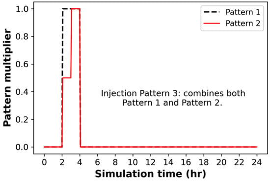
Figure 4.
Injection pattern multiplier for the case study scenarios.

Table 2.
Characteristics of case study scenarios.
Various source locations of contaminant injection were tested for the different designed patterns, as outlined in Table 2. For the EPANET Net3 network, the injection locations were selected based on the work by Seth et al. [20], and the same criteria were applied when choosing the injection locations for the Richmond network. It should be noted that specific sites were selected for the Net3 and Richmond networks to be near water quality sensors. These sites, namely 151 (Net3) and 91 (Richmond network), are covered by a single sensor (refer to Figure 2 and Figure 3). Conversely, sites 189 (Net3) and 518 (Richmond network) were deliberately chosen to be located far away from water quality sensor locations, covered by two sensors (refer to Figure 2 and Figure 3).
The EPANET injection source type was chosen as a “set point booster” for all the above scenarios. Furthermore, the contaminant was assumed to be subjected to both bulk and wall reaction coefficients in all scenarios, unless stated otherwise. For the candidate solutions, the objective function values for the single injection were set to be below 10%, and for multiple contamination injections, less than 15%. These value thresholds serve as benchmarks. The device used to conduct the simulations for all scenarios has the following configuration: ASUS VivoBook, Model: S512F, Intel Core i5-10th processor, 12 GB of memory, and Windows 10–64-bit operating system.
5. Results and Discussion
5.1. Sensitivity Analysis and Hyperparameter Tuning
First, we focus on investigating the influence of the choice of surrogate model and acquisition function on the accuracy and computational efficiency of the BO CSI framework. To that end, we tested two different probabilistic surrogate models, namely Gaussian Process (GP) regression and Random Forest (RF) regression, in combination with three acquisition functions: probability of improvement (POI), expected improvement (EI), and Upper Confidence Bound (UCB). To conduct this sensitivity analysis, Scenario A is selected as the basis, which involves a single intrusion location (node 189 in the Net3 network) and a dosage of 1000 mg/L. For this sensitivity analysis, the injected contaminant was assumed to be conservative.
5.1.1. Choice of the GP Covariance Kernel Function
The investigated methods have several crucial hyperparameters that require tuning. First, in the case of the Gaussian Process (GP) surrogate model, different covariance kernel options were tested to identify the best-performing covariance function for estimating the GP model, namely (a) squared-exponential, (b) Matérn 3/2, (c) gamma-exponential, and (d) rational quadratic.
The length scale parameter plays a critical role in characterizing the smoothness of the GP surrogate function, and thus affects the accuracy of the GP model in fitting the underlying objective function. To select the optimal length scale (OLS) for each kernel, the five-fold cross-validation mean squared error (CV_MSE) resulting from fitting each kernel to 1000 randomly generated evaluations of the objective function was minimized by means of a univariate bounded optimization routine, namely the minimize_scalar function in the scipy library.
Figure 5 illustrates the CV_MSE of the GP surrogate model (y-axis) at different values of the length scale parameter (x-axis) for the four kernels. The figure highlights the significance of selecting appropriate length scale values for each kernel, as the accuracy of the GP model in predicting the objective function values varies significantly across different length scale values. The following optimal length scale values and their respective CV_MSE values were obtained for each kernel function: 3.74 → 45.37 for the SE kernel, 18.52 → 31.41 for M32, 816.07 → 618.16 for GE, and 5.70 → 30.19 for RQ. Based on these findings, it can be concluded that the RQ kernel yields the lowest CV_MSE value, indicating a higher accuracy in fitting the GP surrogate model. Therefore, a further analysis was continued using the rational quadratic kernel (GP_RQ).

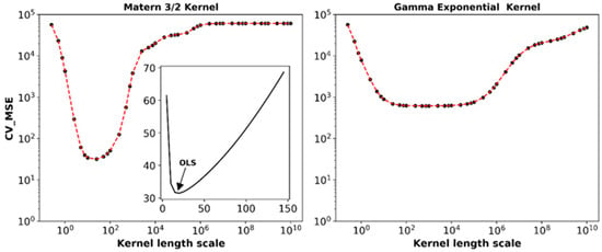
Figure 5.
Cross-validation MSE of the GP regression model vs. the length scale of the four covariance kernels. OLS = optimal length scale.
5.1.2. Number of Initial Evaluations
Another important parameter that requires tuning is the number of initial evaluations used to fit the prior of the probabilistic surrogate model. To determine the optimal number of initial evaluations, a wide range was tested for both surrogate models (GP_RQ and RF), starting from 0 to 1000 with an increment of 20. Figure 6 shows the cross-validation r2 values calculated for both of the surrogate models using different numbers of initial evaluations. As expected, increasing the number of initial evaluations improves the performance of the surrogate model in fitting the objective function. However, increasing the number of initial evaluations also increases the computational cost of fitting the models. As a result, we concluded that selecting 400 initial evaluations for GP_RQ and 500 initial evaluations for RF provides a satisfactory trade-off between accuracy and computational cost.
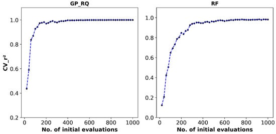
Figure 6.
Cross-validation r2 of the two surrogate models vs. the number of initial evaluations used to fit the models.
5.1.3. Choice of the Surrogate Model and Acquisition Function
Following the choice of the GP covariance kernel, optimal length scale values, and number of initial evaluations, we tested the performance of both surrogate models in conjunction with three acquisition functions, namely POI, EI, and UCB. Three different metrics were used in this comparison: the best objective function, total runtime, and convergence profile. The objective function value reflects the quality of the obtained solution through each method, while the total runtime reflects the computational cost of training the surrogate model and performing the optimization iterations. The convergence profile revealed the rate at which the optimization converged toward the best solution.
Figure 7 depicts the value of the best objective function achieved through each surrogate model-acquisition function combination after 200 iterations. The results show that the GP surrogate model generally produces solutions of a significantly lower quality compared to the RF model with the three acquisition function alternatives. Furthermore, RF was able to consistently identify the source location along with the exact start and end times when employed with all tested acquisition functions as listed in Table 3, far surpassing the performance of the GP alternatives.
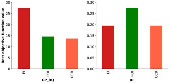
Figure 7.
The best objective function achieved using different BO surrogate models and acquisition functions.

Table 3.
Results of different BO Surrogate Models and Acquisition Functions for Scenario A.
Next, we examined the total runtime of each of the tested BO methods, which is crucial in facilitating a rapid response to contamination events. The findings show that the GP model options require more computational time than the RF model alternatives (Table 3). Among the GP alternatives, GP_UCB utilized the most time, specifically 15.68 min/node for 200 iterations, whereas GP_EI and GP_POI required less time (Table 3). This was consistent with the results of previous literature, where Candelieri et al. [35] deduced that BO with GP models demands an average of 7.5 times the wall clock time needed for RF-based BO. Among the RF alternatives, both RF_UCB and RF_EI combinations required slightly lower computational time than the other options, with RF_UCB showing the best computational efficiency.
Finally, we examined the convergence profile of the different BO methods, which gauges the ability of BO to rapidly guide the search space toward convergence. The results depicted in Figure 8 show that, in general, the GP alternatives converge slower than the RF combinations. Notably, both RF_UCB and RF_EI quickly acquire and achieve the assumed parameters of Scenario A within a minimal number of iterations (19), corresponding to approximately 0.33 and 0.39 min/node, respectively.
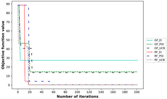
Figure 8.
Convergence profiles of different BO surrogate models and acquisition functions.
Taken together, the results of the sensitivity analysis revealed that the Random Forest (RF) regression surrogate model remarkably outperformed the Gaussian Process (GP) regression surrogate model, which can be attributed to two key factors: (1) Since RF regression relies on building multiple decision trees and averaging their predictions, it can capture a wide range of data patterns, which makes it very effective at capturing nonlinear relationships between features and the target variable. (2) RF regression has built-in mechanisms, such as bootstrapping and averaging, to prevent overfitting, which makes it more robust, especially when dealing with noisy data.
Additionally, the results also revealed that the influence of the acquisition function on the performance of BO is less significant than that of the surrogate model. This is also consistent with recent studies that investigated the application of BO for water quality optimization [44]. However, comparing the performance of the three acquisition functions, the UCB function achieved the best value for the objective function when coupled with both surrogate models (Figure 7). Furthermore, UCB converged to the best solution in fewer iterations than both POI and EI (Figure 8). Nevertheless, UCB required more computational time when coupled with the GP surrogate model (Table 3).
5.2. Influence of Pattern, Location, and Number of Sources
Overall, the Random Forest (RF) surrogate model in conjunction with the Upper Confidence Bound (UCB) acquisition function displayed the best performance, in terms of both accuracy and convergence speed. Hence, the RF_UCB combination was selected for a further analysis in this study.
5.2.1. Continuous Injection
Figure 9 illustrates the patterns of the best solutions achieved using the selected BO method (RF-UCB) in comparison with the true injection characteristics for Scenarios A–D. The four scenarios feature continuous injection pattern 1 on both the Net3 WDS (Scenarios A and B) and Richmond WDS (Scenarios C and D). For each scenario, the figure depicts the top four candidate solutions produced using the BO algorithm as well as the true injection scenario. For all four scenarios, the best solution achieved using BO (dashed green line) matched the true injection scenario (solid cyan line) almost exactly in terms of starting time and duration, and was able to find the true injection location, but with very slight differences in the mass loading rate. Generally, the BO algorithm required less than 100 iterations to converge to the best solution in all four scenarios.
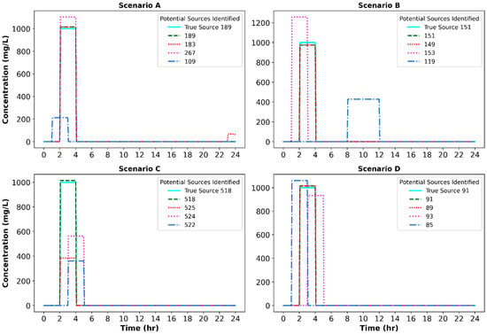
Figure 9.
True contamination source and top solutions achieved using BO for the continuous injection pattern.
As can be observed in Figure 9, the second top candidate solution for all scenarios, except Scenario C, was in good agreement with the true injection scenario. Nevertheless, as listed in Table 4, significant differences existed between the objective function values of the best and the second-best solutions. Thus, the algorithm was able to identify the right solution with little confusion.

Table 4.
Objective function values for the top two candidate solutions for the continuous pattern.
5.2.2. Non-Uniform Contaminant Injection
Figure 10 reveals the top four optimal solutions that the BO algorithm identified for Scenarios E-H, all featuring non-uniform injection pattern 2. The green dashed line represents the overall best solution for all scenarios, while the true source pattern is represented by the cyan solid line. For the four injection scenarios, the RF_UCB algorithm was able to identify the true injection source locations, durations, and contaminant mass amounts with fairly high accuracy. It is also worth noting that Scenario B and F, and Scenario D and H, true injection locations were designed to be adjacent to the sensor location, which explains why they show a good agreement between the top first and second candidate solutions for both Patterns 1 and 2. However, this is not the case for Scenarios C and G, and Scenarios A and E, given that they were designed to be distant from the sites of the sensors.
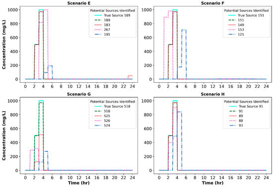
Figure 10.
True contamination source and top solutions achieved using BO for the non-uniform injection pattern.
It is also worth mentioning that Pattern 2, designed to be more complex than Pattern 1, required 150 iterations to reduce the initial objective function from 489.57% to 2.11% as can be seen from Table 5. The average time taken to reach the optimal solution was 2.82 min per node for the Net3 network and 4.95 min per node for the Richmond network. Due to its higher complexity, the Richmond network required more time for EPANET simulation of the hydraulic and water quality analysis compared to the Net3 network. Despite the significant difference in the initial objective function error of the best solutions between the Richmond and Net3 networks, the BO-based framework achieved low error values for both networks (Table 5).

Table 5.
Objective function values for the top two candidate solutions for the non-uniform pattern.
5.2.3. Multiple Injection Locations
Pattern 3 was designed to incorporate combinations of Pattern 1 and Pattern 2. This involved testing two simultaneous contaminant injections at nodes 151 and 189 for Scenario J and nodes 91 and 518 for Scenario K. Nodes 151 and 91 represented Pattern 1, while nodes 189 and 518 represented Pattern 2. Table 6 presents the characteristics of the top five candidate combination solutions. It took 200 iterations for both networks to reduce the objective function target value to 6.34% for Scenario J and 5.44% for Scenario K (Table 6).

Table 6.
Results of contamination sources at multiple injection locations.
The RF_UCB model successfully identified the locations of contaminant injection for both networks. The results in Table 6 indicate that the most likely sources were candidate nodes 151 and 189 for Scenario J and 91 and 518 for Scenario K. This deduction is based on the fact that all other candidate combinations returned final objective function values above 6.34% for the Net3 network and 5.44% for the Richmond network.
The algorithm achieved slightly more accurate results for the complex Richmond Water Network compared to the smaller Net3 network, as the achieved function value in the Richmond network was slightly lower than in the Net3 network. However, the time required to reach the target error was 3.81 min/node for Net3 and 6.23 min/node for Richmond. The significant time difference can be attributed to two factors. The first is the size of the water distribution network as EPANET required more time to simulate the hydraulic and water quality simulation for the larger Richmond network. The second is the total duration of the simulation for Richmond that was twice that of the Net3 network.
The results depicted in Table 6 also indicate that the algorithm accurately identified the injection duration, location, simulated concentrations for the uniform pattern, and first simulated dosage for the doubled pattern. However, in the second doubled pattern, the simulated dosage in both networks was slightly higher than the assumed value in the true pattern (500 mg/L). Although the RF_UCB model performs well in identifying the two simultaneous injection sites, it performs much better in finding a single injection characteristic.
5.3. Influence of Measurement Uncertainty and Contaminant Reaction
In this section, we focus on understanding the robustness of the BO model by introducing two variations: measurement error in the sensors and assuming a decay reaction for the contaminant. A study by Seth et al. [20] highlighted that monitoring errors can significantly influence the performance of CSI frameworks. Additionally, according to Hart et al. [45], one of the major sources of uncertainty in water quality modeling is the type and reaction dynamics. Herein, we examined the Richmond network’s five designed pattern scenarios (Scenario C, Scenario D, Scenario G, Scenario H, and Scenario K).
Two performance metrics were utilized to evaluate every result scenario the selected BO algorithm generates: accuracy and specificity. These metrics were established by Yang and Boccelli [11] to evaluate their proposed model, and later used by Seth et al. [20] to compare the performance of three CSI methods. Accuracy measures the extent to which the algorithm accurately identifies the actual contaminant source(s) as the most likely source(s). Specificity determines how effectively the BO model narrows down the range of candidate nodes.
In this case, the corresponding inverse of the objective function error for each candidate solution represents the likeliness measure of each node identified in that solution. It is worth noting that 100 percent accuracy means that the true injection node had the highest likeliness value, while a high specificity value indicates that the true injection node ranks the highest among all candidate nodes.
To test the robustness of the algorithm to measurement errors, a random normally distributed noise was generated and added to the measured data at the designated sensor locations to assess the robustness of the selected simulation–optimization approach.
where represents the observed concentrations at sensor location i, represents the observed concentrations with error at sensor location i, represents the normal distribution random error, and represents the error magnitude. The chosen error magnitude is designed to simulate a high level of measurement error. Figure 11 demonstrates the difference between the shape of observed concentrations with and without adding noise to Pattern 1.
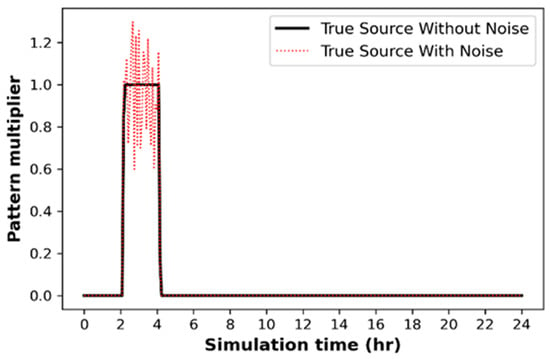
Figure 11.
Injection pattern 1 with and without the addition of sensor measurement noise.
Figure 12 demonstrates that the selected model (RF_UCB Bayesian optimization) performs well in the presence of sensor noise for all designed scenarios, achieving 100% accuracy and specificity. However, it is worth noting that the objective function value of the second top candidate solution is closer to the best solution, which is not true for previous scenarios involving non-reactive contaminant reactions. Guan et al. [13] also found that their simulation–optimization method successfully identified the true contamination source in the presence of measurement error.
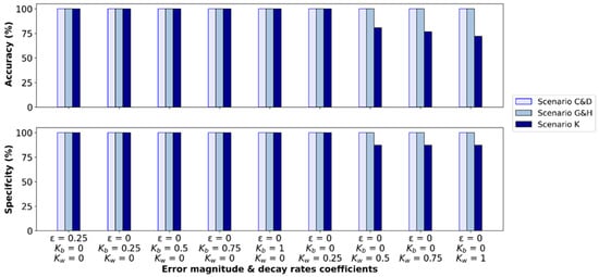
Figure 12.
Accuracy and specificity results for Richmond network considering sensor noise and contaminant decay.
Next, two types of decay reaction rate coefficients are considered to examine the model’s accuracy. They are bulk and wall reaction rate coefficients Kb and Kw, respectively. The first exemplifies a constant rate for reactions occurring in the bulk flow, while the second is a pipe–wall reaction coefficient. The test assumes first-order reactions occurring in both the bulk flow and at the pipe wall. In designing this test, both Kb (day−1) and Kw (m/day) were selected to follow the set range [0.25, 0.5, 0.75, 1].
Figure 12 shows that the proposed BO model successfully identifies the assumed contamination sources in the case of a single contamination source for Patterns 1 and 2, with all different permutations. In Scenario K, which involves two simultaneous injections, the model achieves 100% accuracy and specificity, except when the Kw values range from 0.5 to 1 m/day (Figure 12). The results indicate that higher values of Kw slightly decrease accuracy. Conversely, the Kb coefficient does not significantly impact accuracy or specificity. Two main factors are responsible for increasing the contribution and influence of the Kw factor: a higher flow velocity and smaller pipe diameter. At a higher wall decay constant, the wall rate coefficient accounts for the majority of total chlorine decay (loss), which explains why Kw has a greater effect on the model’s ability to identify the correct solution than Kb.
5.4. Limitations and Recommendations for Further Development
The Bayesian optimization CSI model demonstrated remarkable robustness in handling diverse water network complexities and pattern injection scenarios, with high accuracy and specificity in revealing the true characteristics of multiple contamination sources. In the future, several key areas of improvement for the BO model should be investigated.
First, it is essential to acknowledge the limitations in EPANET water quality simulation, which could have an effect on the accuracy of the CSI results. These limitations include the numerical errors in the EPANET water quality simulation engine, the limited representation of incomplete mixing at the network junctions, and the implementation of an advection-based transport model rather than an advection–dispersion model that could accurately simulate both Laminar and Turbulent flow regimes [46]. The latter is known to affect the results of water quality optimization analyses, especially in the low-flow, dead-end zones of WDSs [47].
Second, the examination and comparison of different surrogate models, such as Gradient Boosting and T-student, can present an opportunity for enhancing the model’s capabilities. Evaluating the performance of other surrogate models against the presented RF_UCB model can provide valuable insights into potential improvements in CSI performance. Furthermore, optimizing the trade-off between exploration and exploitation within the acquisition functions is essential for achieving better performance in a shorter timeframe. Striking the right balance between these aspects is crucial to expedite the convergence to optimal solutions.
Third, it is crucial to investigate how the presented CSI framework can be expanded into a complete contamination response framework that combines CSI with the optimization of response strategies. One possible approach to achieve this linkage is by incorporating the presented CSI within real-time water quality control frameworks [48]. The latter may also include other components, such as the optimization of booster chlorination systems [49,50].
Finally, it is worth investigating how the performance of the presented BO framework compares to the performance of machine learning-based CSI approaches, such as Random Forests and Neural Networks. This comparison will reveal the role of the acquisition function formulation in driving the search for the optimal solution in BO. This comparison will also help shed light on how the performance of simulation–optimization approaches compares to that of direct simulation approaches involving data-driven models.
6. Conclusions
In the event of accidental or intentional contamination in the drinking water distribution system (WDS), it is crucial to quickly identify the contaminant source characteristics to maintain high water quality and protect public health. These characteristics include spatial location, duration, and concentration of the contaminant injection source. In this study, a closed-loop simulation–optimization approach was developed to solve this inverse, black-box, computationally expensive problem. Bayesian optimization (BO) served as the optimization engine for the contamination source identification (CSO) framework, while EPANET (WNTR) was used to simulate hydraulics and water quality dynamics within the WDS.
A comprehensive comparison of various BO surrogate models and acquisition functions was conducted. To demonstrate the proposed CSI framework, two different case study WDSs, with different sizes and complexities, were employed. The investigation included various injection patterns and locations. Overall, the presented BO framework achieved outstanding performance in finding the contamination source characteristics for all designated scenarios. The findings revealed that BO with Random Forest (RF) regression as the surrogate model and the Upper Confidence Bound (UCB) as the acquisition function demonstrated the most effective performance in identifying contamination source(s) quickly and with minimal evaluations.
To further evaluate the robustness of the proposed model, two uncertainty factors were considered: noise added at monitoring stations and a decay reaction for the injected contaminant. Random errors in sensor measurement data did not impact the determination of source patterns for all analyzed scenarios. Furthermore, the proposed approach effectively identified contamination sources when both bulk and wall decay reactions were considered for the small WDS. However, high wall decay rates appeared to negatively impact the performance of the BO CSI framework, especially when the size of the WDS is large.
In summary, Bayesian optimization is a promising approach for identifying contamination source(s) in drinking water distribution networks. Continued research in this area will help address the identified limitations and fully implement this approach in practical contamination response frameworks, which will significantly enhance our ability to respond swiftly and effectively to water contamination events, ensuring the safety and reliability of community drinking water systems.
Author Contributions
Conceptualization, K.A. and A.A.A.; methodology, K.A.; software, K.A.; validation, K.A. and A.A.A.; formal analysis, K.A.; investigation, K.A.; resources, K.A.; data curation, K.A.; writing—original draft preparation, K.A.; writing—review and editing, K.A. and A.A.A.; visualization, K.A.; supervision, A.A.A.; project administration, K.A. and A.A.A.; funding acquisition, A.A.A. All authors have read and agreed to the published version of the manuscript.
Funding
This research was Supported by the National Science Foundation (NSF) under Grant No. 2015603.
Data Availability Statement
The data presented in this study are available upon request from the corresponding author.
Acknowledgments
Support from the NSF is gratefully acknowledged.
Conflicts of Interest
The authors declare no conflict of interest.
References
- Abokifa, A.A.; Sela, L. Identification of spatial patterns in water distribution pipe failure data using spatial autocorrelation analysis. J. Water Resour. Plan. Manag. 2019, 145, 04019057. [Google Scholar] [CrossRef]
- Bello, O.; Abu-Mahfouz, A.M.; Hamam, Y.; Page, P.R.; Adedeji, K.B.; Piller, O. Solving management problems in water distribution networks: A survey of approaches and mathematical models. Water 2019, 11, 562. [Google Scholar] [CrossRef]
- Menapace, A.; Zanfei, A.; Felicetti, M.; Avesani, D.; Righetti, M.; Gargano, R. Burst detection in water distribution systems: The issue of dataset collection. Appl. Sci. 2020, 10, 8219. [Google Scholar] [CrossRef]
- Taha, A.F.; Wang, S.; Guo, Y.; Summers, T.H.; Gatsis, N.; Giacomoni, M.H.; Abokifa, A.A. Revisiting the water quality sensor placement problem: Optimizing network observability and state estimation metrics. J. Water Resour. Plan. Manag. 2021, 147, 04021040. [Google Scholar] [CrossRef]
- Tryby, M.E.; Propato, M.; Ranjithan, S.R. Monitoring Design for Source Identification in Water Distribution Systems. J. Water Resour. Plan. Manag. 2010, 136, 637–646. [Google Scholar] [CrossRef]
- Aral, M.M.; Guan, J.; Maslia, M.L. Optimal Design of Sensor Placement in Water Distribution Networks. J. Water Resour. Plan. Manag. 2010, 136, 5–18. [Google Scholar] [CrossRef]
- Krause, A.; Leskovec, J.; Guestrin, C.; VanBriesen, J.; Faloutsos, C. Efficient Sensor Placement Optimization for Securing Large Water Distribution Networks. J. Water Resour. Plan. Manag. 2008, 134, 516–526. [Google Scholar] [CrossRef]
- Preis, A.; Ostfeld, A. Multiobjective Contaminant Sensor Network Design for Water Distribution Systems. J. Water Resour. Plan. Manag. 2008, 134, 366–377. [Google Scholar] [CrossRef]
- Xu, J.; Fischbeck, P.S.; Small, M.J.; VanBriesen, J.M.; Casman, E. Identifying Sets of Key Nodes for Placing Sensors in Dynamic Water Distribution Networks. J. Water Resour. Plan. Manag. 2008, 134, 378–385. [Google Scholar] [CrossRef]
- Propato, M.; Tryby, M.E.; Piller, O. Linear algebra analysis for contaminant source identification in water distribution systems. In Proceedings of the World Environmental and Water Resources Congress 2007: Restoring Our Natural Habitat, 2007 ASCE, Tampa, FL, USA, 15–19 May 2007; pp. 1–10. [Google Scholar]
- Yang, X.; Boccelli, D.L. Bayesian Approach for Real-Time Probabilistic Contamination Source Identification. J. Water Resour. Plan. Manag. 2014, 140, 04014019. [Google Scholar] [CrossRef]
- Laird, C.D.; Biegler, L.T.; van Bloemen Waanders, B.G.; Bartlett, R.A. Contamination Source Determination for Water Networks. J. Water Resour. Plan. Manag. 2005, 131, 125–134. [Google Scholar] [CrossRef]
- Guan, J.; Aral, M.M.; Maslia, M.L.; Grayman, W.M. Identification of Contaminant Sources in Water Distribution Systems Using Simulation–Optimization Method: Case Study. J. Water Resour. Plan. Manag. 2006, 132, 252–262. [Google Scholar] [CrossRef]
- Preis, A.; Ostfeld, A. Contamination Source Identification in Water Systems: AHybrid Model Trees–Linear Programming Scheme. J. Water Resour. Plan. Manag. 2006, 132, 263–273. [Google Scholar] [CrossRef]
- De Sanctis, A.E.; Shang, F.; Uber, J.G. Real-Time Identification of Possible Contamination Sources Using Network Backtracking Methods, J. Water Resour. Plan. Manag. 2010, 136, 444–453. [Google Scholar]
- Berglund, E.Z.; Pesantez, J.E.; Rasekh, A.; Shafiee, M.E.; Sela, L.; Haxton, T. Review of Modeling Methodologies for Managing Water Distribution Security, J. Water Resour. Plan. Manag. 2020, 146, 03120001. [Google Scholar]
- Liu, L.; Ranjithan, S.R.; Mahinthakumar, G. Contamination Source Identification in Water Distribution Systems Using an Adaptive Dynamic Optimization Procedure. J. Water Resour. Plan. Manag. 2011, 137, 183–192. [Google Scholar] [CrossRef]
- Hu, C.; Zhao, J.; Yan, X.; Zeng, D.; Guo, S. A MapReduce based Parallel Niche Genetic Algorithm for contaminant source identification in water distribution network. Ad Hoc Netw. 2015, 35, 116–126. [Google Scholar] [CrossRef]
- Grbčić, L.; Lučin, I.; Kranjčević, L.; Družeta, S. Water supply network pollution source identification by random forest algorithm. J. Hydroinform. 2020, 22, 1521–1535. [Google Scholar] [CrossRef]
- Seth, A.; Klise, K.A.; Siirola, J.D.; Haxton, T.; Laird, C.D. Testing Contamination Source Identification Methods for Water Distribution Networks. J. Water Resour. Plan. Manag. 2016, 142, 04016001. [Google Scholar] [CrossRef]
- Rossman, L.A. EPANET 2 Users Manual EPA/600/R-00/57; United States Environmental Protection Agency: Cincinnati, OH, USA, 2000.
- Archetti, F.; Candelieri, A. Bayesian Optimization and Data Science; Springer: Berlin/Heidelberg, Germany, 2019. [Google Scholar]
- Frazier, P.I. A Tutorial on Bayesian Optimization. arXiv 2018, arXiv:1807.02811. [Google Scholar]
- Shahriari, B.; Swersky, K.; Wang, Z.; Adams, R.P.; De Freitas, N. Taking the human out of the loop: A review of Bayesian optimization. Proc. IEEE. 2016, 104, 148–175. [Google Scholar] [CrossRef]
- Chen, Y.; Huang, A.; Wang, Z.; Antonoglou, I.; Schrittwieser, J.; Silver, D.; de Freitas, N. Bayesian Optimization in AlphaGo. arXiv 2018, arXiv:1812.06855. [Google Scholar]
- Nguyen, V.; Osborne, M.A. Knowing the what but not the where in Bayesian optimization. In Proceedings of the 37th International Conference on Machine Learning, PMLR, Virtual, 13–18 July 2020; Volume 119, pp. 7317–7326. [Google Scholar]
- Pelikan, M.; Goldberg, D.; Cantu-Paz, E. BOA: The Bayesian Optimization Algorithm (IlliGAL Report No. 99003); University of Illinois at Urbana-Champaign: Urbana, IL, USA, 1999. [Google Scholar]
- Snoek, J.; Larochelle, H.; Adams, R.P. Practical Bayesian optimization of machine learning algorithms. Adv. Neural Inf. Process. Syst. 2012, 4, 2951–2959. [Google Scholar]
- Frazier, P.I.; Wang, J. Bayesian Optimization for Materials Design; Springer Series in Materials Science; Springer: Berlin/Heidelberg, Germany, 2015; pp. 45–75. [Google Scholar]
- Nogueira, J.; Martinez-Cantin, R.; Bernardino, A.; Jamone, L. Unscented Bayesian optimization for safe robot grasping. In Proceedings of the 2016 IEEE/RSJ International Conference on Intelligent Robots and Systems (IROS), Daejeon, Republic of Korea, 9–14 October 2016; pp. 1967–1972. [Google Scholar]
- Pyzer-Knapp, E.O. Bayesian optimization for accelerated drug discovery. IBM J. Res. Dev. 2018, 62, 1–7. [Google Scholar] [CrossRef]
- Klise, K.; Hart, D.; Bynum, M.; Hogge, J. Water Network Tool for Resilience (WNTR) User Manual; U.S. Environmental Protection Agency: Washington, DC, USA, 2017.
- Jiménez, J.; Ginebra, J. pyGPGO: Bayesian Optimization for Python. J. Open Source Softw. 2017, 2, 431. [Google Scholar] [CrossRef]
- Coello Coello, C.A. (Ed.) Learning and Intelligent Optimization; Lecture Notes in Computer Science; Springer: Berlin/Heidelberg, Germany, 2011. [Google Scholar]
- Candelieri, A.; Perego, R.; Archetti, F. Bayesian optimization of pump operations in water distribution systems. J. Glob. Optim. 2018, 71, 213–235. [Google Scholar] [CrossRef]
- Melkumyan, A.; Nettleton, E. An observation angle dependent nonstationary covariance function for Gaussian process regression. In Neural Information Processing: 16th International Conference, ICONIP 2009, Bangkok, Thailand, 1–5 December 2009, Proceedings, Part I 16; Lecture Notes in Computer Science (Including Subseries Lecture Notes in Artificial Intelligence and Lecture Notes in Bioinformatics); Springer: Berlin/Heidelberg, Germany, 2009; pp. 331–339. [Google Scholar]
- Han, J.; Kamber, M.; Pei, J. Data Mining: Concepts and Techniques; Classification Basic Concepts 8; Elsevier Science: Amsterdam, The Netherlands, 2012. [Google Scholar]
- Hastie, T.; Tibshirani, R.; Friedman, J. The Elements of Statistical Learning; Springer Series in Statistics; Springer: New York, NY, USA, 2009. [Google Scholar]
- Jones, D.R. ATaxonomy of Global Optimization Methods Based on Response Surfaces. J. Glob. Optim. 2001, 21, 345–383. [Google Scholar] [CrossRef]
- Agrawal, T. Hyperparameter Optimization in Machine Learning: Make Your Machine Learning and Deep Learning Models More Efficient; Apress: Bangalore, India, 2021. [Google Scholar]
- Auer, P. Using Confidence Bounds for Exploitation-Exploration Trade-offs. J. Mach. Learn. Res. 2002, 3, 26. [Google Scholar]
- Kaufmann, E.; Cappé, O.; Garivier, A. On Bayesian upper confidence bounds for bandit problems. J. Mach. Learn. Res. 2012, 22, 592–600. [Google Scholar]
- Preis, A.; Ostfeld, A. Genetic algorithm for contaminant source characterization using imperfect sensors. Civ. Eng. Environ. Syst. 2008, 25, 29–39. [Google Scholar] [CrossRef]
- Moeini, M.; Sela, L.; Taha, A.F.; Abokifa, A.A. Bayesian Optimization of Booster Disinfection Scheduling in Water Distribution Networks. Water Res. 2023, 242, 120117. [Google Scholar] [CrossRef] [PubMed]
- Hart, D.; Rodriguez, J.S.; Burkhardt, J.; Borchers, B.; Laird, C.; Murray, R.; Klise, K.; Haxton, T. Quantifying Hydraulic Water Quality Uncertainty to Inform Sampling of Drinking Water Distribution Systems. J. Water Resour. Plan. Manag. 2019, 145, 04018084. [Google Scholar] [CrossRef] [PubMed]
- Abokifa, A.A.; Xing, L.; Sela, L. Investigating the impacts of water conservation on water quality in distribution networks using an advection-dispersion transport model. Water 2020, 12, 1033. [Google Scholar] [CrossRef]
- Abokifa, A.A.; Maheshwari, A.; Gudi, R.D.; Biswas, P. Influence of dead-end sections of drinking water distribution networks on optimization of booster chlorination systems. J. Water Resour. Plan. Manag. 2019, 145, 04019053. [Google Scholar] [CrossRef]
- Wang, S.; Taha, A.F.; Abokifa, A.A. How effective is model predictive control in real-time water quality regulation? State-space modeling and scalable control. Water Resour. Res. 2021, 57, e2020WR027771. [Google Scholar] [CrossRef]
- Maheshwari, A.; Abokifa, A.A.; Gudi, R.D.; Biswas, P. Coordinated decentralization-based optimization of disinfectant dosing in large-scale water distribution networks. J. Water Resour. Plan. Manag. 2018, 144, 04018066. [Google Scholar] [CrossRef]
- Maheshwari, A.; Abokifa, A.; Gudi, R.D.; Biswas, P. Optimization of disinfectant dosage for simultaneous control of lead and disinfection-byproducts in water distribution networks. J. Environ. Manag. 2020, 276, 111186. [Google Scholar] [CrossRef]
Disclaimer/Publisher’s Note: The statements, opinions and data contained in all publications are solely those of the individual author(s) and contributor(s) and not of MDPI and/or the editor(s). MDPI and/or the editor(s) disclaim responsibility for any injury to people or property resulting from any ideas, methods, instructions or products referred to in the content. |
© 2023 by the authors. Licensee MDPI, Basel, Switzerland. This article is an open access article distributed under the terms and conditions of the Creative Commons Attribution (CC BY) license (https://creativecommons.org/licenses/by/4.0/).
