
Retrieving Soil Moisture from Sentinel-1: Limitations over Certain Crops and Sensitivity to the First Soil Thin Layer

 ,
,  , ,
, ,  ,
,  and
and 
Abstract
:1. Introduction
- The consistency between the S1-estimated soil moisture by S2MP and the conventional soil moisture measurements made at a 10 cm depth along a crop cycle/year.
- The limitation of the S1 SM estimations for developed vegetation cover, considering common winter crops and summer irrigated crops (wheat, soybean, tomato and cover crops).
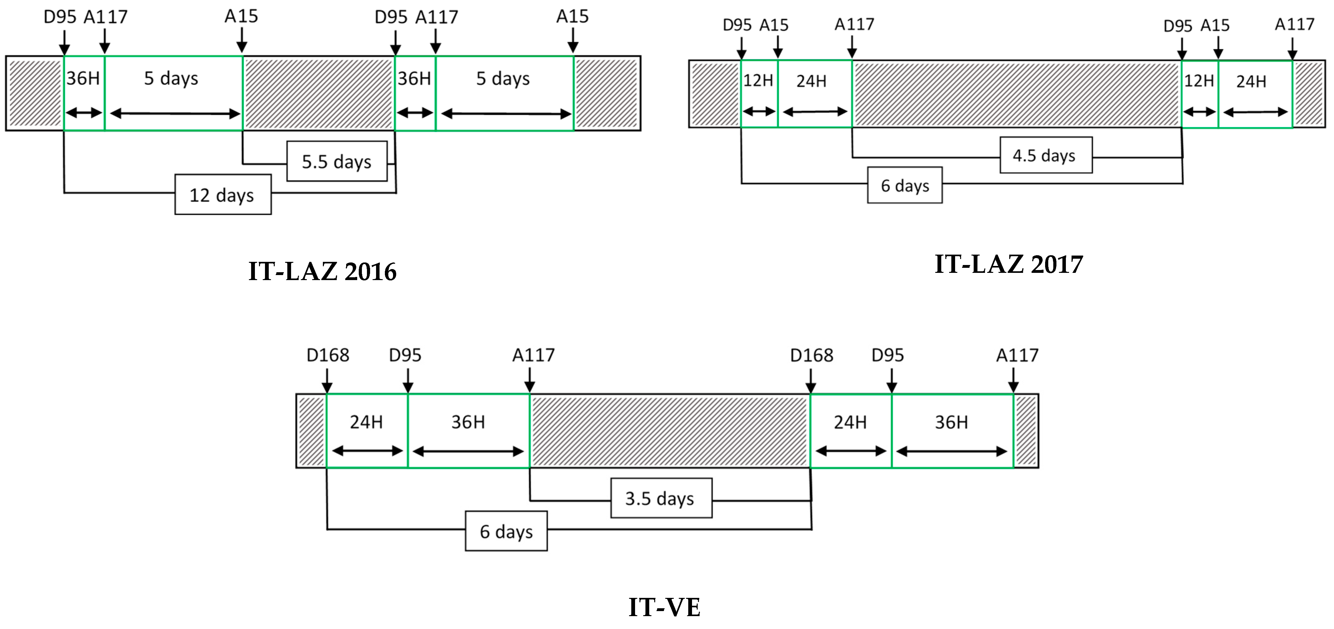
- Evaluate the effect of the S1 acquisition configuration (S1 incidence angle) on the S1 SM estimations.
2. Materials and Methods
2.1. Study Sites
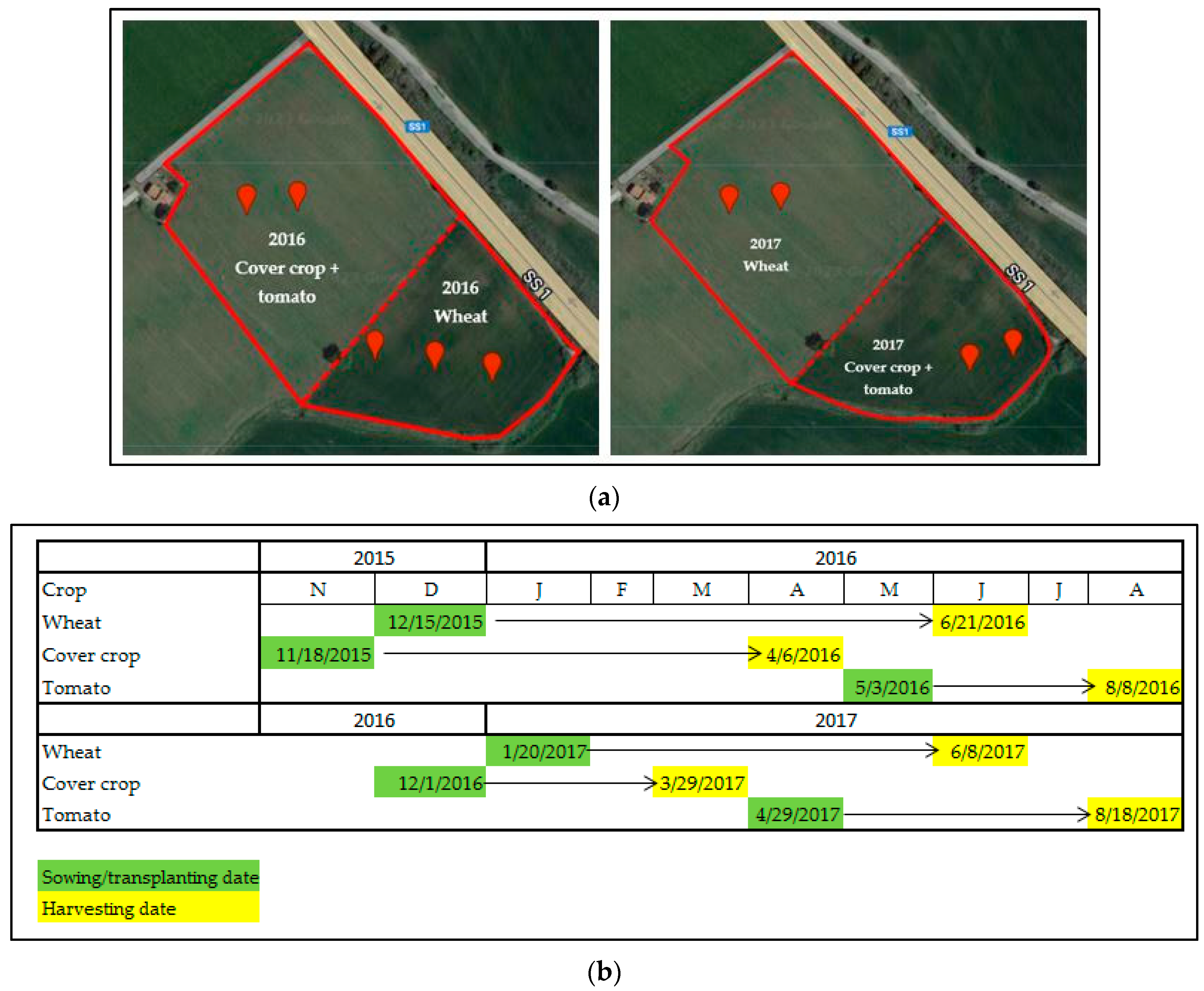
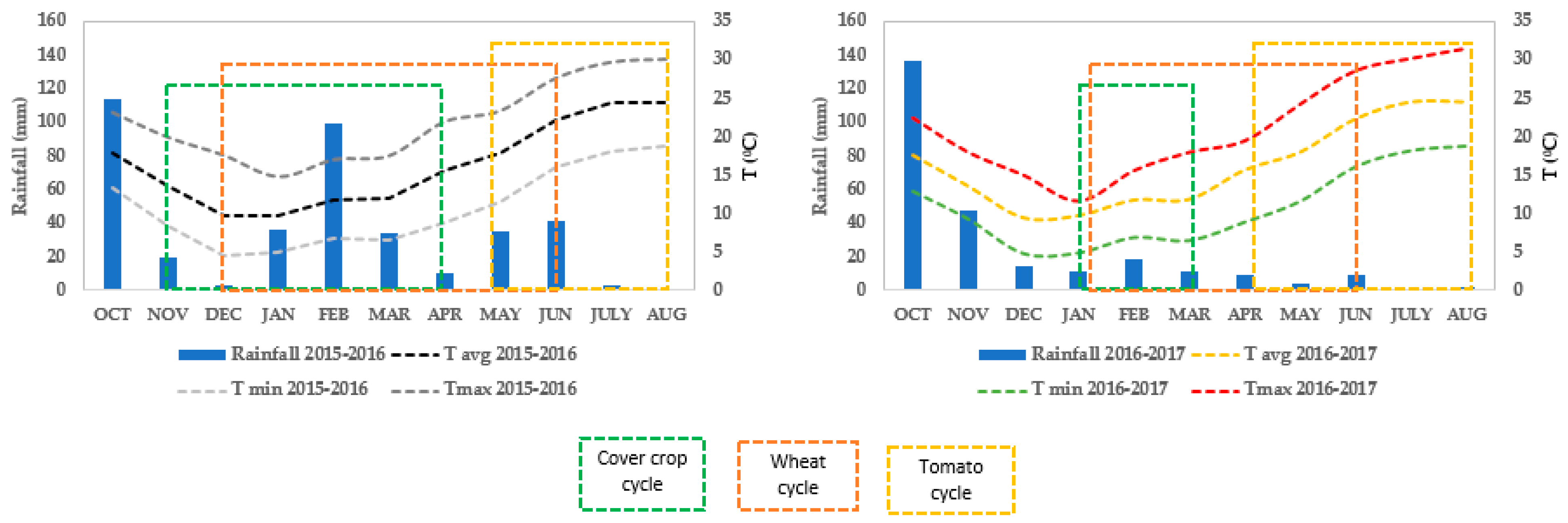
2.1.1. IT-LAZ
- -
- In situ SM data at 10 cm
- -
- Temperature and precipitation data
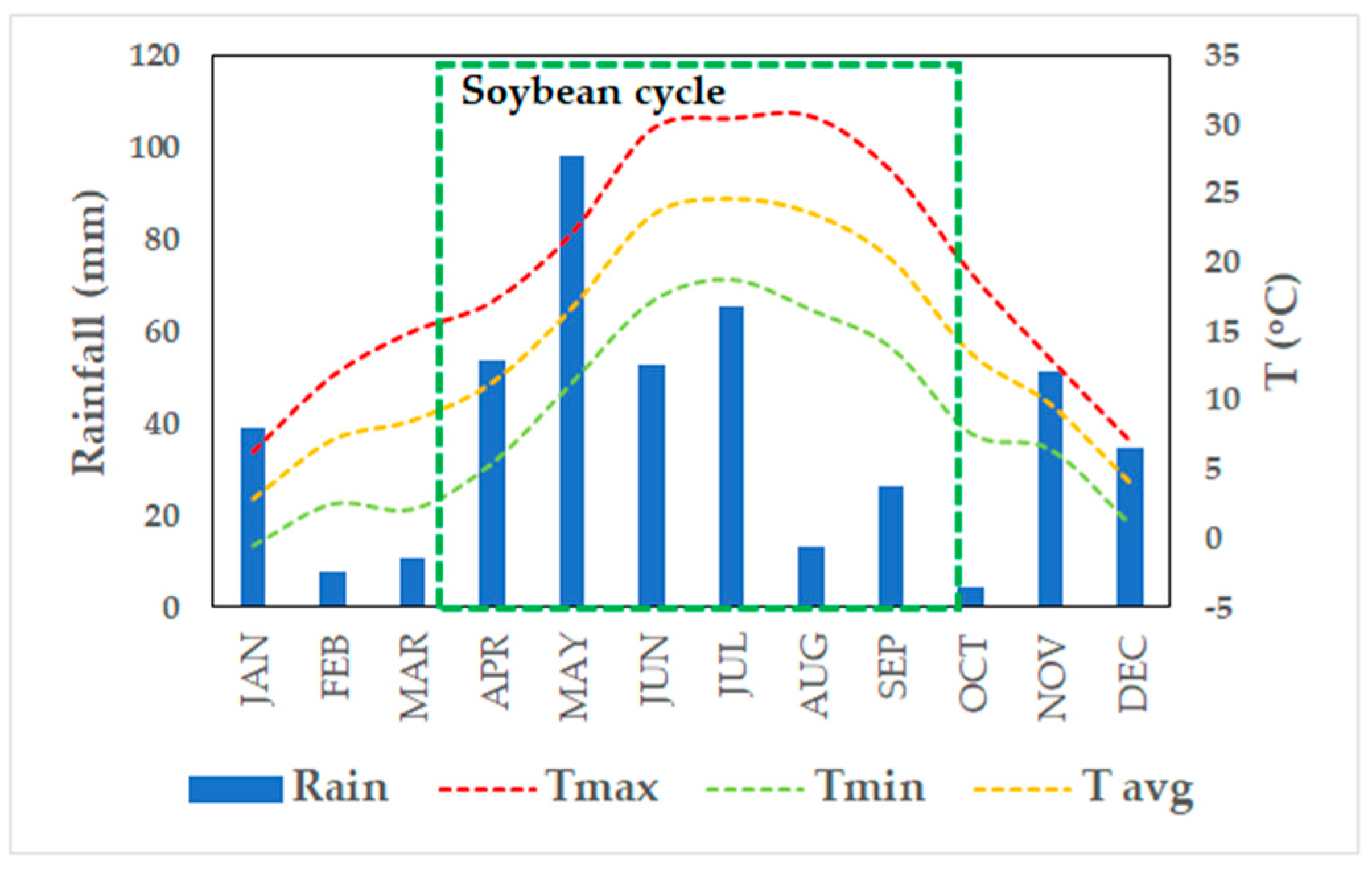
2.1.2. IT-VE
- -
- In situ MS data at 10 cm
- -
- Temperature and precipitation data
2.2. S2MP Soil Moisture
2.3. Methods
3. Results
3.1. Temporal Series Analysis
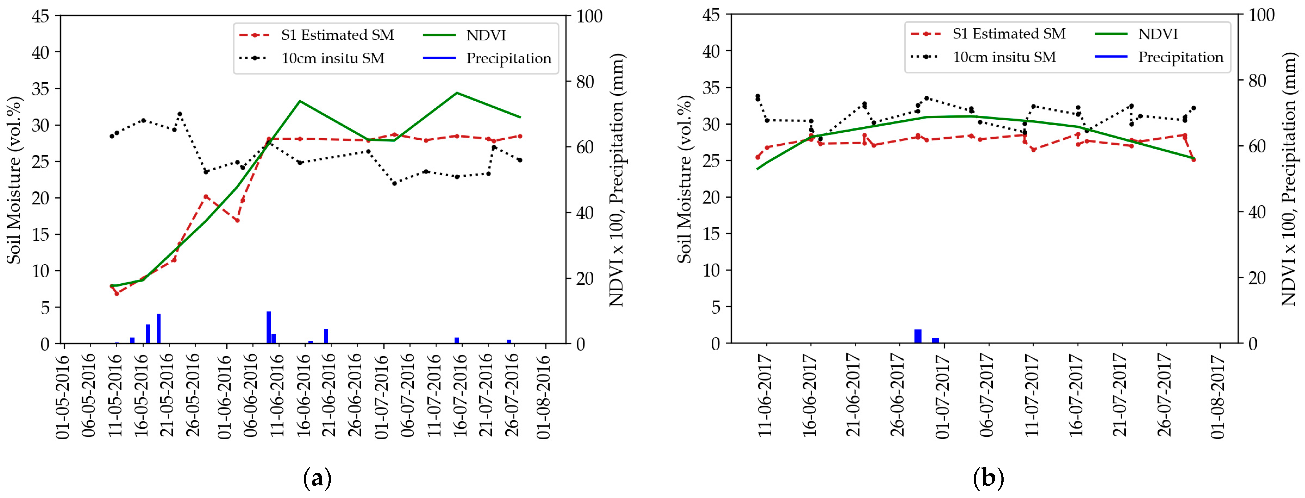
3.1.1. Tomato Crop Case
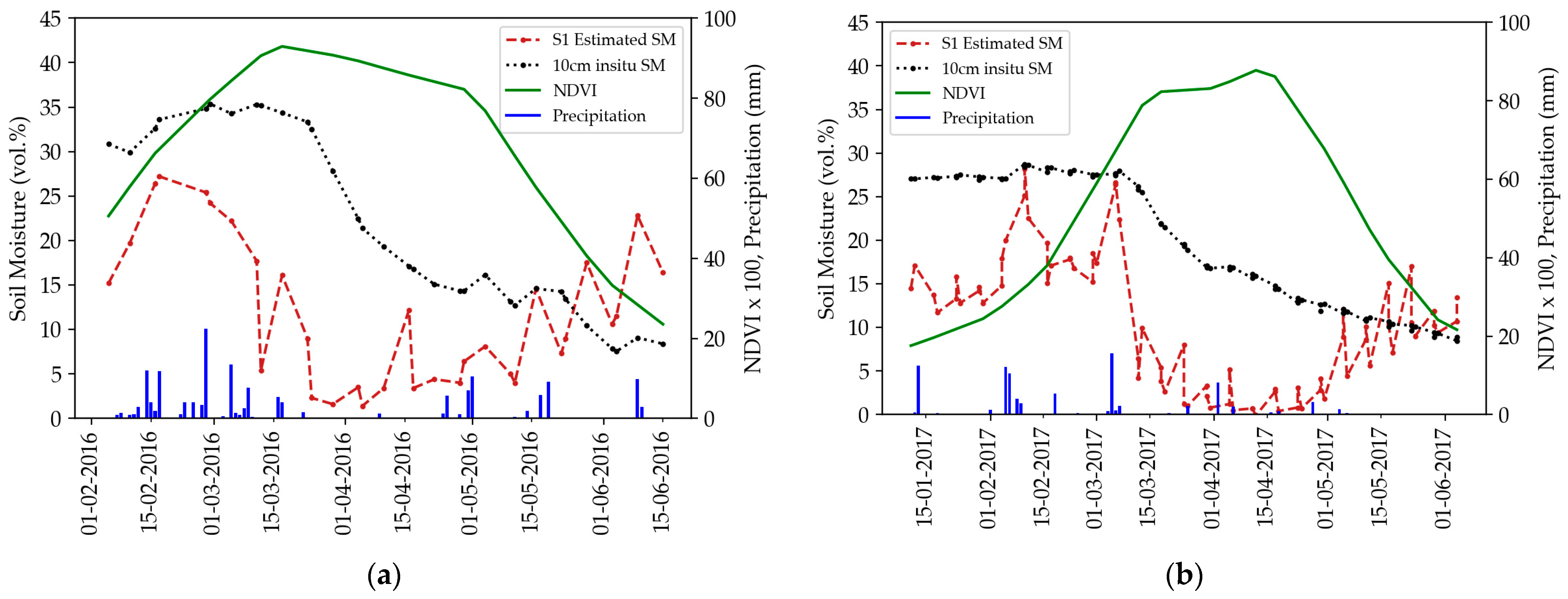
3.1.2. Wheat Crop Case
3.1.3. Cover Crop Case
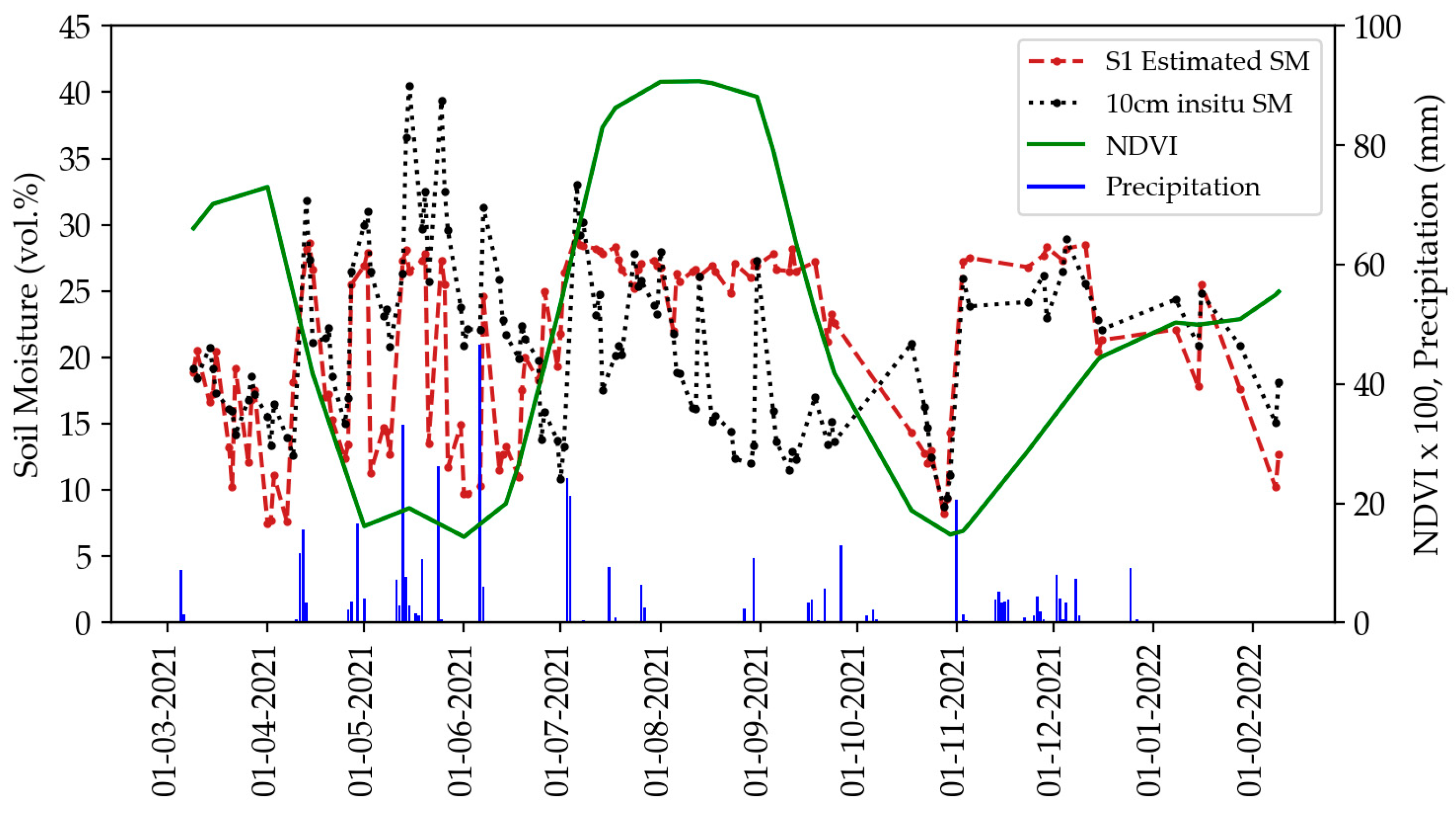
3.1.4. Soybean Crop Case
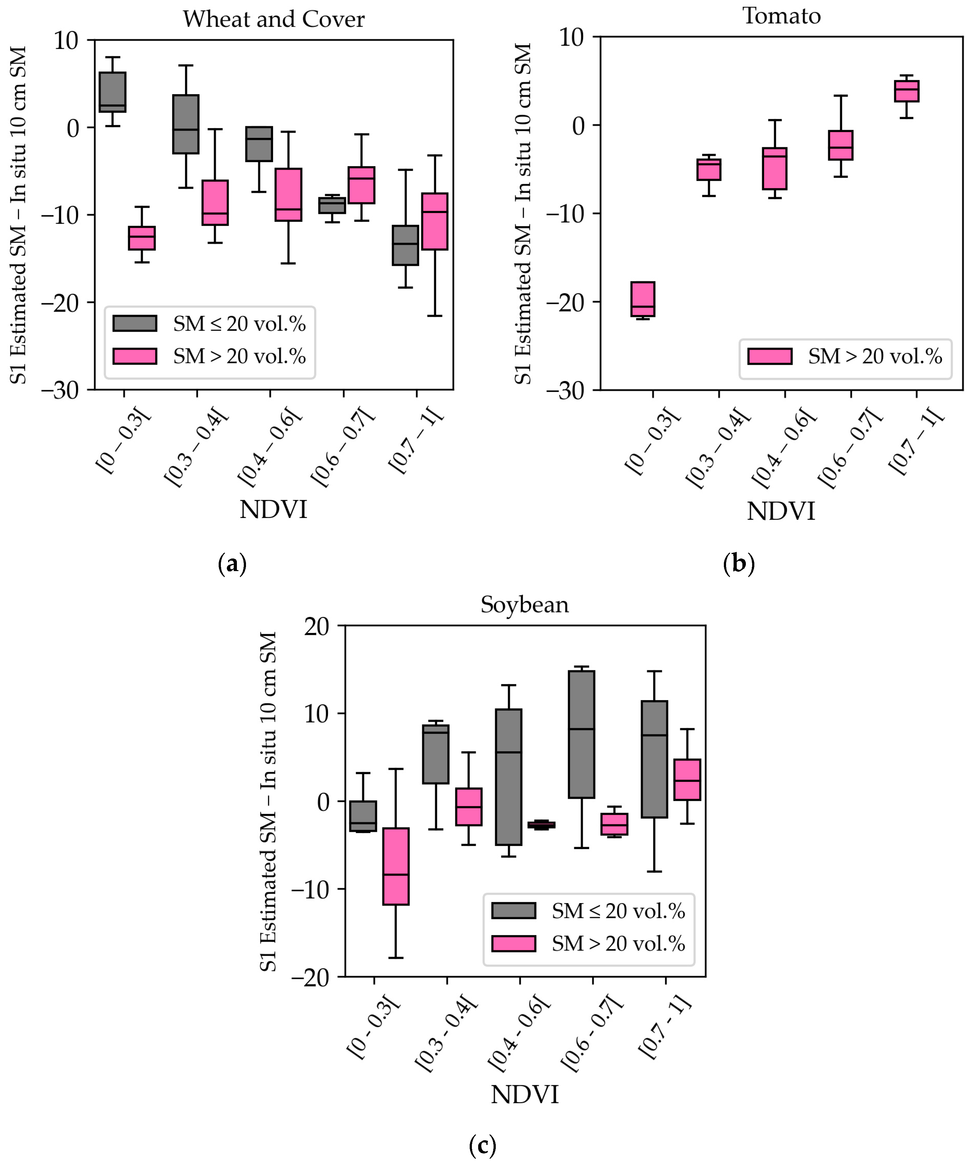
3.2. Differences between Measured and Estimated SM
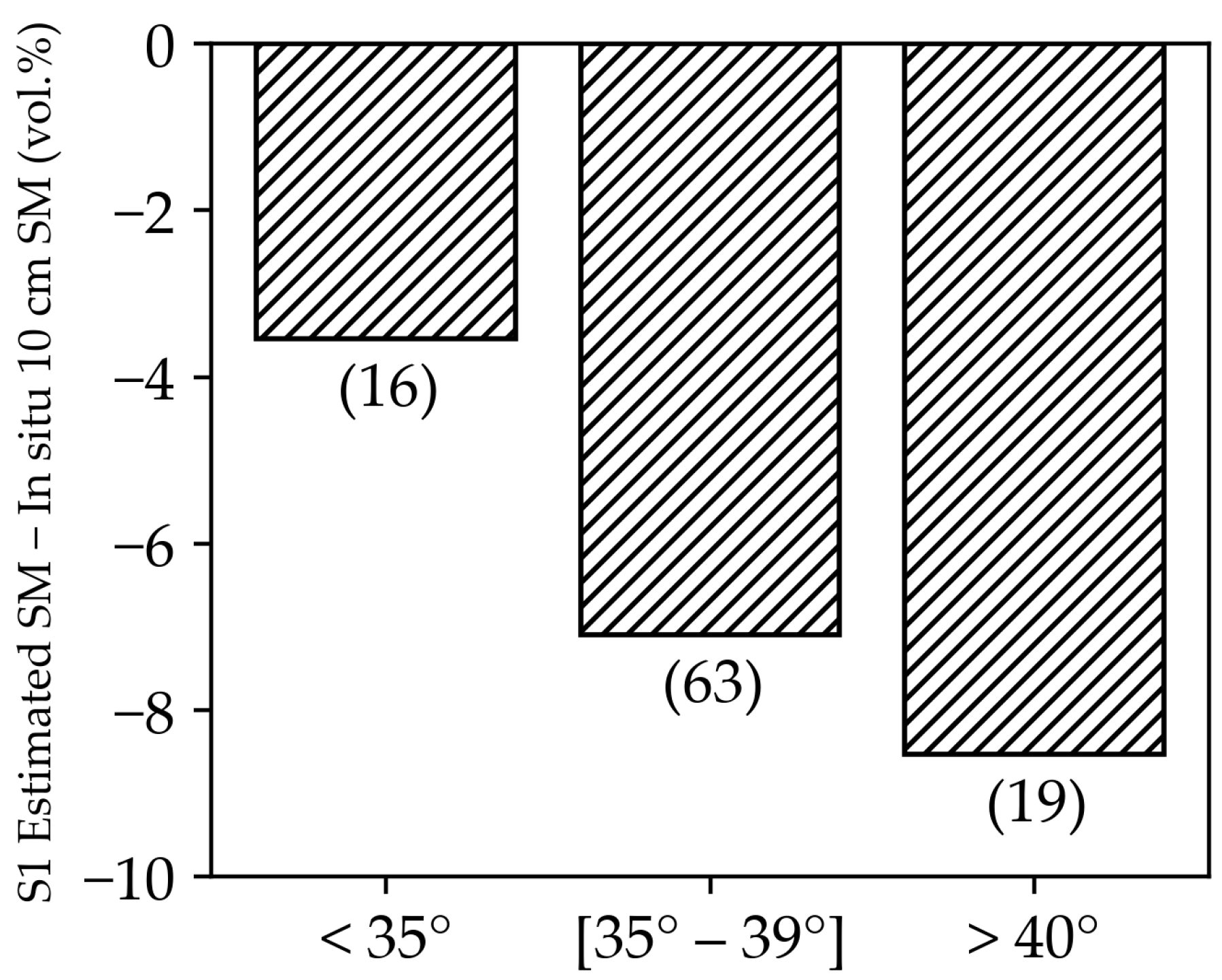
3.3. Effect of the Radar Incidence Angle
4. Discussion
4.1. Soil Moisture at Different Depth Layers
4.2. Limitations of S1 SM Estimations
4.3. Vegetation Effect on S1 SM Retrievals and Recommendation for End Users
5. Conclusions
Author Contributions
Funding
Data Availability Statement
Acknowledgments
Conflicts of Interest
References
- Massari, C.; Modanesi, S.; Dari, J.; Gruber, A.; De Lannoy, G.J.M.; Girotto, M.; Quintana-Seguí, P.; Le Page, M.; Jarlan, L.; Zribi, M.; et al. A Review of Irrigation Information Retrievals from Space and Their Utility for Users. Remote Sens. 2021, 13, 4112. [Google Scholar] [CrossRef]
- Quast, R.; Wagner, W.; Bauer-Marschallinger, B.; Vreugdenhil, M. Soil Moisture Retrieval from Sentinel-1 Using a First-Order Radiative Transfer Model—A Case-Study over the Po-Valley. Remote Sens. Environ. 2023, 295, 113651. [Google Scholar] [CrossRef]
- Bauer-Marschallinger, B.; Freeman, V.; Cao, S.; Paulik, C.; Schaufler, S.; Stachl, T.; Modanesi, S.; Massari, C.; Ciabatta, L.; Brocca, L.; et al. Toward Global Soil Moisture Monitoring with Sentinel-1: Harnessing Assets and Overcoming Obstacles. IEEE Trans. Geosci. Remote Sens. 2019, 57, 520–539. [Google Scholar] [CrossRef]
- El Hajj, M.; Baghdadi, N.; Zribi, M.; Bazzi, H. Synergic Use of Sentinel-1 and Sentinel-2 Images for Operational Soil Moisture Mapping at High Spatial Resolution over Agricultural Areas. Remote Sens. 2017, 9, 1292. [Google Scholar] [CrossRef]
- Entekhabi, D.; Njoku, E.G.; O’Neill, P.E.; Kellogg, K.H.; Crow, W.T.; Edelstein, W.N.; Entin, J.K.; Goodman, S.D.; Jackson, T.J.; Johnson, J.; et al. The Soil Moisture Active Passive (SMAP) Mission. Proc. IEEE 2010, 98, 704–716. [Google Scholar] [CrossRef]
- Kerr, Y.H.; Waldteufel, P.; Wigneron, J.-P.; Martinuzzi, J.; Font, J.; Berger, M. Soil Moisture Retrieval from Space: The Soil Moisture and Ocean Salinity (SMOS) Mission. IEEE Trans. Geosci. Remote Sens. 2001, 39, 1729–1735. [Google Scholar] [CrossRef]
- Wagner, W.; Hahn, S.; Kidd, R.; Melzer, T.; Bartalis, Z.; Hasenauer, S.; Figa-Saldana, J.; De Rosnay, P.; Jann, A.; Schneider, S.; et al. The ASCAT Soil Moisture Product: A Review of Its Specifications, Validation Results, and Emerging Applications. Meteorol. Z. 2013, 22, 5–33. [Google Scholar] [CrossRef]
- Wigneron, J.-P.; Li, X.; Frappart, F.; Fan, L.; Al-Yaari, A.; De Lannoy, G.; Liu, X.; Wang, M.; Le Masson, E.; Moisy, C. SMOS-IC Data Record of Soil Moisture and L-VOD: Historical Development, Applications and Perspectives. Remote Sens. Environ. 2021, 254, 112238. [Google Scholar] [CrossRef]
- Kornelsen, K.C.; Coulibaly, P. Advances in Soil Moisture Retrieval from Synthetic Aperture Radar and Hydrological Applications. J. Hydrol. 2013, 476, 460–489. [Google Scholar] [CrossRef]
- Singh, A.; Gaurav, K. Deep Learning and Data Fusion to Estimate Surface Soil Moisture from Multi-Sensor Satellite Images. Sci. Rep. 2023, 13, 2251. [Google Scholar] [CrossRef]
- Singh, S.K.; Prasad, R.; Srivastava, P.K.; Yadav, S.A.; Yadav, V.P.; Sharma, J. Incorporation of First-Order Backscattered Power in Water Cloud Model for Improving the Leaf Area Index and Soil Moisture Retrieval Using Dual-Polarized Sentinel-1 SAR Data. Remote Sens. Environ. 2023, 296, 113756. [Google Scholar] [CrossRef]
- Das, N.N.; Entekhabi, D.; Dunbar, R.S.; Chaubell, M.J.; Colliander, A.; Yueh, S.; Jagdhuber, T.; Chen, F.; Crow, W.; O’Neill, P.E.; et al. The SMAP and Copernicus Sentinel 1A/B Microwave Active-Passive High Resolution Surface Soil Moisture Product. Remote Sens. Environ. 2019, 233, 111380. [Google Scholar] [CrossRef]
- Bazzi, H.; Baghdadi, N.; El Hajj, M.; Zribi, M.; Belhouchette, H. A Comparison of Two Soil Moisture Products S2MP and Copernicus-SSM Over Southern France. IEEE J. Sel. Top. Appl. Earth Obs. Remote Sens. 2019, 12, 3366–3375. [Google Scholar] [CrossRef]
- Fan, J.; Han, Q.; Tan, S.; Li, J. Evaluation of Six Satellite-Based Soil Moisture Products Based on in Situ Measurements in Hunan Province, Central China. Front. Environ. Sci. 2022, 10, 829046. [Google Scholar] [CrossRef]
- Escorihuela, M.J.; Quintana-Seguí, P. Comparison of Remote Sensing and Simulated Soil Moisture Datasets in Mediterranean Landscapes. Remote Sens. Environ. 2016, 180, 99–114. [Google Scholar] [CrossRef]
- Ullmann, T.; Jagdhuber, T.; Hoffmeister, D.; May, S.M.; Baumhauer, R.; Bubenzer, O. Exploring Sentinel-1 Backscatter Time Series over the Atacama Desert (Chile) for Seasonal Dynamics of Surface Soil Moisture. Remote Sens. Environ. 2023, 285, 113413. [Google Scholar] [CrossRef]
- Baghdadi, N.; Cerdan, O.; Zribi, M.; Auzet, V.; Darboux, F.; El Hajj, M.; Kheir, R.B. Operational Performance of Current Synthetic Aperture Radar Sensors in Mapping Soil Surface Characteristics in Agricultural Environments: Application to Hydrological and Erosion Modelling. Hydrol. Process. 2008, 22, 9–20. [Google Scholar] [CrossRef]
- El Hajj, M.; Baghdadi, N.; Bazzi, H.; Zribi, M. Penetration Analysis of SAR Signals in the C and L Bands for Wheat, Maize, and Grasslands. Remote Sens. 2019, 11, 31. [Google Scholar] [CrossRef]
- Gao, Q.; Zribi, M.; Escorihuela, M.; Baghdadi, N. Synergetic Use of Sentinel-1 and Sentinel-2 Data for Soil Moisture Mapping at 100 m Resolution. Sensors 2017, 17, 1966. [Google Scholar] [CrossRef]
- Vanino, S.; Nino, P.; De Michele, C.; Falanga Bolognesi, S.; D’Urso, G.; Di Bene, C.; Pennelli, B.; Vuolo, F.; Farina, R.; Pulighe, G.; et al. Capability of Sentinel-2 Data for Estimating Maximum Evapotranspiration and Irrigation Requirements for Tomato Crop in Central Italy. Remote Sens. Environ. 2018, 215, 452–470. [Google Scholar] [CrossRef]
- Stevanato, L.; Baroni, G.; Cohen, Y.; Fontana, C.L.; Gatto, S.; Lunardon, M.; Marinello, F.; Moretto, S.; Morselli, L. A Novel Cosmic-Ray Neutron Sensor for Soil Moisture Estimation over Large Areas. Agriculture 2019, 9, 202. [Google Scholar] [CrossRef]
- Gianessi, S.; Polo, M.; Stevanato, L.; Lunardon, M.; Francke, T.; Oswald, S.; Ahmed, H.; Tolosa, A.; Weltin, G.; Dercon, G.; et al. Testing a Novel Sensor Design to Jointly Measure Cosmic-Ray Neutrons, Muons and Gamma Rays for Non-Invasive Soil Moisture Estimation. Geosci. Instrum. Method. Data Syst. Discuss. 2022; in review. [Google Scholar] [CrossRef]
- El Hajj, M.; Baghdadi, N.; Zribi, M.; Rodríguez-Fernández, N.; Wigneron, J.; Al-Yaari, A.; Al Bitar, A.; Albergel, C.; Calvet, J.-C. Evaluation of SMOS, SMAP, ASCAT and Sentinel-1 Soil Moisture Products at Sites in Southwestern France. Remote Sens. 2018, 10, 569. [Google Scholar] [CrossRef]
- Baghdadi, N.; El Hajj, M.; Zribi, M.; Bousbih, S. Calibration of the Water Cloud Model at C-Band for Winter Crop Fields and Grasslands. Remote Sens. 2017, 9, 969. [Google Scholar] [CrossRef]
- Bazzi, H.; Baghdadi, N.; Charron, F.; Zribi, M. Comparative Analysis of the Sensitivity of SAR Data in C and L Bands for the Detection of Irrigation Events. Remote Sens. 2022, 14, 2312. [Google Scholar] [CrossRef]
- Benninga, H.-J.F.; van der Velde, R.; Su, Z. Soil Moisture Content Retrieval over Meadows from Sentinel-1 and Sentinel-2 Data Using Physically Based Scattering Models. Remote Sens. Environ. 2022, 280, 113191. [Google Scholar] [CrossRef]
- Ulaby, F.T.; Moore, R.K.; Fung, A.K. Microwave Remote Sensing: Active and Passive. Volume 3—From Theory to Applications; Artech House: London, UK, 1986. [Google Scholar]
- Bruckler, L.; Witono, H.; Stengel, P. Near Surface Soil Moisture Estimation from Microwave Measurements. Remote Sens. Environ. 1988, 26, 101–121. [Google Scholar] [CrossRef]
- Zhu, L.; Walker, J.P.; Ye, N.; Rüdiger, C. Roughness and Vegetation Change Detection: A Pre-Processing for Soil Moisture Retrieval from Multi-Temporal SAR Imagery. Remote Sens. Environ. 2019, 225, 93–106. [Google Scholar] [CrossRef]
- Dong, L.; Baghdadi, N.; Ludwig, R. Validation of the AIEM Through Correlation Length Parameterization at Field Scale Using Radar Imagery in a Semi-Arid Environment. IEEE Geosci. Remote Sens. Lett. 2013, 10, 461–465. [Google Scholar] [CrossRef]
- Grote, K.; Anger, C.; Kelly, B.; Hubbard, S.; Rubin, Y. Characterization of Soil Water Content Variability and Soil Texture Using GPR Groundwave Techniques. J. Environ. Eng. Geophys. 2010, 15, 93–110. [Google Scholar] [CrossRef]
- Dabrowska-Zielinska, K.; Musial, J.; Malinska, A.; Budzynska, M.; Gurdak, R.; Kiryla, W.; Bartold, M.; Grzybowski, P. Soil Moisture in the Biebrza Wetlands Retrieved from Sentinel-1 Imagery. Remote Sens. 2018, 10, 1979. [Google Scholar] [CrossRef]
- Balenzano, A.; Mattia, F.; Satalino, G.; Lovergine, F.P.; Palmisano, D.; Peng, J.; Marzahn, P.; Wegmüller, U.; Cartus, O.; Dąbrowska-Zielińska, K.; et al. Sentinel-1 Soil Moisture at 1 Km Resolution: A Validation Study. Remote Sens. Environ. 2021, 263, 112554. [Google Scholar] [CrossRef]
- Ma, C.; Li, X.; McCabe, M.F. Retrieval of High-Resolution Soil Moisture through Combination of Sentinel-1 and Sentinel-2 Data. Remote Sens. 2020, 12, 2303. [Google Scholar] [CrossRef]
- Arias, M.; Notarnicola, C.; Campo-Bescós, M.Á.; Arregui, L.M.; Álvarez-Mozos, J. Evaluation of Soil Moisture Estimation Techniques Based on Sentinel-1 Observations over Wheat Fields. Agric. Water Manag. 2023, 287, 108422. [Google Scholar] [CrossRef]
- Morrison, K.; Wagner, W. Explaining Anomalies in SAR and Scatterometer Soil Moisture Retrievals from Dry Soils with Subsurface Scattering. IEEE Trans. Geosci. Remote Sens. 2020, 58, 2190–2197. [Google Scholar] [CrossRef]
- Wagner, W.; Lindorfer, R.; Melzer, T.; Hahn, S.; Bauer-Marschallinger, B.; Morrison, K.; Calvet, J.-C.; Hobbs, S.; Quast, R.; Greimeister-Pfeil, I.; et al. Widespread Occurrence of Anomalous C-Band Backscatter Signals in Arid Environments Caused by Subsurface Scattering. Remote Sens. Environ. 2022, 276, 113025. [Google Scholar] [CrossRef]
- Aubert, M.; Baghdadi, N.N.; Zribi, M.; Ose, K.; El Hajj, M.; Vaudour, E.; Gonzalez-Sosa, E. Toward an Operational Bare Soil Moisture Mapping Using TerraSAR-X Data Acquired Over Agricultural Areas. IEEE J. Sel. Top. Appl. Earth Obs. Remote Sens. 2013, 6, 900–916. [Google Scholar] [CrossRef]
- Bazzi, H.; Baghdadi, N.; Najem, S.; Jaafar, H.; Le Page, M.; Zribi, M.; Faraslis, I.; Spiliotopoulos, M. Detecting Irrigation Events over Semi-Arid and Temperate Climatic Areas Using Sentinel-1 Data: Case of Several Summer Crops. Agronomy 2022, 12, 2725. [Google Scholar] [CrossRef]
- Zappa, L.; Schlaffer, S.; Bauer-Marschallinger, B.; Nendel, C.; Zimmerman, B.; Dorigo, W. Detection and Quantification of Irrigation Water Amounts at 500 m Using Sentinel-1 Surface Soil Moisture. Remote Sens. 2021, 13, 1727. [Google Scholar] [CrossRef]
- Modanesi, S.; Massari, C.; Bechtold, M.; Lievens, H.; Tarpanelli, A.; Brocca, L.; Zappa, L.; De Lannoy, G.J.M. Challenges and Benefits of Quantifying Irrigation through the Assimilation of Sentinel-1 Backscatter Observations into Noah-MP. Hydrol. Earth Syst. Sci. 2022, 26, 4685–4706. [Google Scholar] [CrossRef]


| 2015/2016 | 2017 | |||
|---|---|---|---|---|
| Crop | From | To | From | To |
| Wheat | 4-February-16 | 16-June-16 | 11-January-17 | 5-June-17 |
| Cover crop | 10-November-15 | 5-April-16 | 11-January-17 | 29-March-17 |
| Tomato | 5-May-16 | 1-August-16 | 8-June-17 | 2-August-17 |
| Crop Type | Low-to-Moderate Vegetation Cover (NDVI < 0.7) | Developed Vegetation Cover (NDVI ≥ 0.7) | ||||
|---|---|---|---|---|---|---|
| RMSE (vol.%) | Bias (vol.%) | R | RMSE (vol.%) | Bias (vol.%) | R | |
| Wheat | 8.6 | −5.4 | 0.65 | 16.6 | −15.5 | 0.67 |
| Cover crop | 7.0 | −6.1 | 0.01 | 9.4 | −8.9 | 0.37 |
| Tomato | 11.72 | −10.6 | 0.23 | 3.7 | −1.0 | −0.34 |
| Soybean crop | 7.4 | −1.84 | 0.46 | 7.5 | 4.1 | 0.32 |
| All data | 7.9 | −3.9 | 0.59 | 11.5 | −6.0 | 0.48 |
| Crop Type | S1 SM Relevance | Reason for Limitation | Suitable NDVI Interval for SM Estimates |
|---|---|---|---|
| Tomato and similar aboveground vegetables | From beginning of the cycle until fruits’ development | Presence of fruits increases S1 backscattering, causing a slight overestimation of SM | From 0 to 0.7 |
| Wheat and similar straw cereals | From the beginning of the cycle until the gemination phase, and then after the heading phase | Wheat kernels attenuate the S1 backscattering, causing the loss of the soil contribution on the signal | NDVI between 0 and 0.6 |
| Soybean and similar pea-family crops | From the beginning of the cycle until the pod’s development | Bean pods increase the S1 backscattering, causing a high overestimation of SM | NDVI between 0 and 0.6 |
Disclaimer/Publisher’s Note: The statements, opinions and data contained in all publications are solely those of the individual author(s) and contributor(s) and not of MDPI and/or the editor(s). MDPI and/or the editor(s) disclaim responsibility for any injury to people or property resulting from any ideas, methods, instructions or products referred to in the content. |
© 2023 by the authors. Licensee MDPI, Basel, Switzerland. This article is an open access article distributed under the terms and conditions of the Creative Commons Attribution (CC BY) license (https://creativecommons.org/licenses/by/4.0/).
Share and Cite
Bazzi, H.; Baghdadi, N.; Nino, P.; Napoli, R.; Najem, S.; Zribi, M.; Vaudour, E. Retrieving Soil Moisture from Sentinel-1: Limitations over Certain Crops and Sensitivity to the First Soil Thin Layer. Water 2024, 16, 40. https://doi.org/10.3390/w16010040
Bazzi H, Baghdadi N, Nino P, Napoli R, Najem S, Zribi M, Vaudour E. Retrieving Soil Moisture from Sentinel-1: Limitations over Certain Crops and Sensitivity to the First Soil Thin Layer. Water. 2024; 16(1):40. https://doi.org/10.3390/w16010040
Chicago/Turabian StyleBazzi, Hassan, Nicolas Baghdadi, Pasquale Nino, Rosario Napoli, Sami Najem, Mehrez Zribi, and Emmanuelle Vaudour. 2024. "Retrieving Soil Moisture from Sentinel-1: Limitations over Certain Crops and Sensitivity to the First Soil Thin Layer" Water 16, no. 1: 40. https://doi.org/10.3390/w16010040
APA StyleBazzi, H., Baghdadi, N., Nino, P., Napoli, R., Najem, S., Zribi, M., & Vaudour, E. (2024). Retrieving Soil Moisture from Sentinel-1: Limitations over Certain Crops and Sensitivity to the First Soil Thin Layer. Water, 16(1), 40. https://doi.org/10.3390/w16010040