Stability Analysis of Super-Large Special-Shaped Deep Excavation in Coastal Water-Rich Region Considering Spatial Variability of Ground Parameters

Abstract

The excavation of a super-large foundation pit is a greatly risky project in coastal water-rich silt strata, and it is of great significance to establish a numerical model to analyze and predict the stability of the foundation pit retaining its structure for safe construction. Based on a geological investigation report and key node monitoring data, the model parameters have been modified. Subsequently, the random field theory and numerical analysis were employed to proceed with deterministic analysis and uncertainty analysis, respectively. Using the uniform distribution method, Gaussian distribution method and the covariance matrix method to generate a random field model, finite difference software was applied to analyze the impact of spatial variability of cohesion and the internal friction angle on structural deformation. The study shows that the overall distribution of axial force is small on both sides and large in the center, and the axial force is larger near the shaped region. Due to the principle of “lever”, there is a tendency for the horizontal displacement of surrounding piles to partially rebound from the pit when the bearing platform pit is excavated. The spatial variability of the internal friction angle and cohesion has an important influence on the numerical value of the enclosure structure and surface deformation, and the variation pattern is basically unchanged.

1. Introduction

In recent years, with the development of industry and the expansion of cities, the number of high-rise buildings in cities has been increasing, and the depth and scope of deep excavation have been increasing. The rock and soil movement and deformation caused by deep excavation have become increasingly serious, and collapse accidents have also occurred from time to time [1,2,3,4]. According to statistics, among the major building collapse accidents recorded by the Ministry of Construction in the past three years, the pit collapse accidents accounted for about 50% of the total number of collapse accidents, so it is necessary to analyze the stability of the pit and control the deformation of the surrounding strata. Tu et al. [5] studied the impact of excavation in soft soil areas on the support structure and surrounding environment based on a foundation pit in Fuzhou. Based on actual monitoring data, they investigated the changes in the support structure, surrounding buildings, and groundwater level during the excavation process. Wang et al. [6] took a deep foundation pit project in a deep silty clay layer in Hefei as the research object. Using on-site monitoring data, he analyzed the surface settlement of the foundation pit, the deformation of the support structure, the vertical and horizontal displacement of the pile top, the axial force and settlement of the steel support, and the horizontal displacement of the gravity retaining wall on the south side of the foundation pit. Geotechnical engineering design inherently reflects the strong randomness of geotechnical parameters due to its dependence on natural conditions, uncertainty of geotechnical properties and complexity of the engineering environment, etc. Therefore, it is necessary to fully consider the influence of soil spatial variability in foundation stability analysis [7,8,9]. Lumb [10] firstly put forward the concept of “spatial variability” of geotechnical parameters, pointing out that due to the differences in material composition during sedimentation and the role of various uncertain external forces in the later stage, the geotechnical parameters show variability characteristics. Vanmarcke [11,12] developed a random field model describing the spatial variability of soils by considering the soil properties parameters as a random field. Random field modeling of geotechnical parameters is to characterize the spatial variability of the entire soil profile by using a limited number of sample point observations, i.e., reflecting the process of the concrete to the general. Random field computational modeling is proposed to reduce the abstract random field model to the natural state of the soil, reflecting the process from general to specific [13]. With the help of this model, scholars at home and abroad have investigated the effects of spatial variability of soil parameters on foundation-bearing capacity [14], tunnel excavation [15,16,17], deep foundation pit in soft soil [18] and slope stability [19].

The soil, as an engineering material, exhibits significant variability and the properties of different locations within the same soil layer also demonstrate variations. Similarly, the stability of structures or buildings constructed using engineering materials in conjunction with geotechnical bodies, under the influence of spatial variability in engineering material parameters and geotechnical parameters, accompanied by environmental complexity, tends to be unilaterally assessed when deterministic parameters are employed. In recent years, numerous scholars have conducted further investigations into geotechnical uncertainty analysis based on the concepts proposed by Lumb and Vanmarcke. Cheng et al. [20] proposed the utilization of a non-invasive stochastic analysis method to accurately and comprehensively predict the deformation of surrounding rock caused by tunnel excavation, aiming to study the impact of spatial variability in rock mass on such deformation. Cheng et al. [15,21], employing a combination of random field theory and numerical analysis, established a random field model that describes the characteristics of spatial variability in soil parameters using the covariance matrix decomposition method. They also utilized the Monte-Carlo strategy to analyze the influence coefficients of variation in elastic modulus and correlation distances on surface deformation through finite-difference software. Similarly, the random field theory has made outstanding contributions in the measurement of groundwater permeability, mechanical parameters of soft soil and hydrological response [22,23,24].

The current main methods utilized for random field modeling include moving average, discrete Fourier transform, fast Fourier transform and covariance matrix decomposition [25,26,27]. Despite numerous studies conducted by scholars using these methods to analyze the impact of spatial variability of geotechnical body parameters on deformation in geotechnical engineering and ground surface based on the random field theory, many of these research findings remain at a qualitative or semi-quantitative level. Consequently, direct application to engineering design becomes challenging. Therefore, the focus of future research should be directed towards exploring refined methods for evaluating the influence of spatial variability of soil parameters on foundation engineering stability.

2. Basic Theories

2.1. Digital Characterization of Random Fields

The essence of the random field theory is accurately modeling the spatial distribution of geotechnical parameters through chi-squared normally distributed random fields, and characterizing the spatial variability and correlation using variables, correlation function and correlation distance. Consequently, this necessitates an introduction to numerical features in probability statistics and their interconnections.

Let the one-dimensional distribution function of the random field {y(x)} be F(x) and the probability density be f(x), then the mean (mathematical expectation) function of the random field {y(x)} is defined.

The mathematical expectation of $X$ is said to exist if the integral ${\int }_{-\infty }^{+\infty }xf\left(x\right)dx$ converges absolutely and $EX={\int }_{-\infty }^{+\infty }xf\left(x\right)dx$; otherwise, the mathematical expectation of $X$ is said not to exist.

Mathematical expectation is also known as the probability mean and is often referred to simply as expectation or mean. Mathematical expectation is an indicator that characterizes the average state of a random variable, which portrays the centralized location of all possible values of the random variable. The definition of mathematical expectation requires absolute convergence of the series (or integral); otherwise, the expectation is said not to exist. This is because the expected existence of $X$ requires that the order of values of $X$ is independent of the order of $X$; i.e., it requires that any change in the order of $x$ should not change the existence of $EX$, which mathematically requires that the series (or integrals) converge absolutely, and furthermore, absolute convergence has a lot of properties that are also easy to deal with mathematically.

Let $X$ be a random variable, and if $E{\left(X-EX\right)}^2$ exists, then $E{\left(X-EX\right)}^2$ is said to be the variance of $X$, denoted as $DX$ or $Var(X$); i.e., call $\sqrt{DX}$ the standard deviation or mean square deviation of $X$, denoted $\mathsf{\sigma }\left(X\right)$.

The variance of a random variable represents the degree of dispersion and repeatability of its values. The larger the variance, the less repeatable the random variable is, which means that the individual values are less “trustworthy”. Conversely, the smaller the variance, the better the repeatability of the random variable; i.e., the higher the “confidence” in the individual values. At the extreme, if the variance is zero, the random variable is simply a “constant”, with one value representing all values.

If the variance of the random variables $X$ and $Y$ exists and $DX>0$ and $DY>0$, then $E(X-EX)\left(Y-EY\right)]$ is said to be the covariance of the random variables $X$ and $Y$, denoted as $CoV(X,Y)$, i.e.,

$$CoV\left(X,Y\right)=E\left[\left(X-EX\right)\left(Y-EY\right)\right]=E\left(XY\right)-EX·EY$$

(1)

For continuous random variables,

$$E\left(XY\right)={\int }_{-\infty }^{+\infty }{\int }_{-\infty }^{+\infty }xyf\left(x,y\right)dxdy$$

(2)

${\mathsf{\rho }}_{\mathrm{X}\mathrm{Y}}=\frac{\mathrm{C}\mathrm{o}\mathrm{v}(\mathrm{X},\mathrm{Y})}{\sqrt{\mathrm{D}\mathrm{X}}\sqrt{\mathrm{D}\mathrm{Y}}}$ is called the correlation coefficient between random variables $X$ and $Y$. If it is 0, $X$ and $Y$ are said to be uncorrelated; otherwise, they are said to be correlated. The covariance function $CoV(X,Y)$ is essentially the second-order mixed central moments of f(x) and f(y), also known as the self-covariance function; the correlation function ${\rho }_{XY}$ is essentially the second-order mixed moments of the origins of f(x) and f(y), also known as the autocorrelation function, which is generally said to be a binary function of the parameters $X$ and $Y$.

From Equations (1) and (2), there is a close relationship between the covariance $CoV(X,Y)$ and the correlation coefficient ${\rho }_{XY}$; while observing Equation (2), when $X=Y$, the correlation coefficient and the variance are consistent at this point, and it is clear that the variance function can also be derived from the correlation function and the mean value function. Therefore, the most important of the above numerical characteristics are the mean value function and the correlation function. Theoretically, only studying the mean and correlation functions of a random field cannot replace the study of the whole random field, but they do describe the main statistical characteristics of the random field, and they are easier to observe and calculate than the family of exhaustive dimensional distribution functions, so they often play an important role in solving the application of the subject [28].

2.2. Soil Characterization Methods

A better way to represent the spatial variability of soil parameters is the random field model proposed by Vanmarcke to describe the spatial autocorrelation properties of soils. Before introducing the soil characterization method, the concept of variance discount factor is briefly introduced.

Let P denote a point in space and the coordinates of P is (x, y, z), so the stochastic function $Y\left(P\right)=Y(X,Y,Z)$ is called a random field in three-dimensional space. Due to the layered nature of soils during their formation, more attention has been paid to the changes in soil properties along the depth direction in the study of geotechnical problems. It is shown that one-dimensional real chi-squared normal random field simulation of soil profiles is consistent with reality [29]. In this space, the difference between point $Y\left(P\right)$ characteristics is reflected in the standard deviation $\sqrt{DY\left(P\right)}=\sigma$. Similarly, in the standard deviation $\sqrt{D{Y}_h\left(P\right)}={\sigma }_h$ of the spatially averaged characteristic $Y_h\left(P\right)$, as the length of the average h increases; so do the fluctuations in $Y\left(P\right)$ that are cancelled out in doing the spatial averaging operation. Thus, an increase in the length of the average h will cause the standard deviation of the spatially averaged characteristic $\sqrt{D{Y}_h\left(P\right)}$ to decrease. The uncaused ratio of $\sqrt{D{Y}_h\left(P\right)}$ and σ is

$$\Gamma \left(h\right)=\frac{\sqrt{D{Y}_h\left(P\right)}}{\sigma }$$

(3)

Since the function $\Gamma \left(h\right)$ reflects the decay of the standard deviation of the spatially averaged characteristic $\sqrt{D{Y}_h\left(P\right)}$ with respect to the root mean square σ of the point characteristic, the function $\Gamma \left(h\right)$ is the root mean square decay factor. The square of the root means square decay factor; ${\Gamma }^2\left(h\right)$ is the variance discount function [30].

Random field theory uses a variance discount factor to relate soil variability to spatial variability. For a homogeneous soil layer, let $Z$ be a point in the soil layer, then the expression for the soil property index is

$$u\left(Z\right)=\mu +\epsilon \left(Z\right)$$

(4)

where $u\left(Z\right)$ is the soil index at the point; $\mu$ is the calculated point average; $\epsilon \left(Z\right)$ is a random variable.

By the definition of Vanmarcke, it follows that

$$Var\left[u_{∆Z}\right]=Var\left[\tilde{\epsilon }\right]={\sigma }^2{\mathsf{\Gamma }}^2\left(\mathsf{\Delta }Z\right)$$

(5)

where ${\sigma }^2$ is the pointwise variance of $u\left(Z\right)$; ${\mathsf{\Gamma }}^2\left(\mathsf{\Delta }Z\right)$ is the variance reduction factor; $\mathsf{\Delta }Z$ is the sampling spacing; $Var\left[u_{∆Z}\right]$ is the variance that describes the spatial average characteristics at Z. $\tilde{\epsilon }$ is a random variable.

${\mathsf{\Gamma }}^2\left(\mathsf{\Delta }Z\right)$ can be approximated as

$${\mathsf{\Gamma }}^2(\mathsf{\Delta }Z)=\left\{\begin{array}{c}1\hspace{0.25em}\hspace{0.25em}\hspace{0.25em}\hspace{0.25em}(0<\mathsf{\Delta }Z<\mathsf{\Delta }L)\\ \hspace{0.25em}\hspace{0.25em}\hspace{0.25em}\hspace{0.25em}\frac{\mathsf{\Delta }L}{\mathsf{\Delta }Z}\end{array}\right.$$

(6)

where $\mathsf{\Delta }L$ is the soil correlation distance.

From the above equation, the variance discount factor depends on the correlation distance $\mathsf{\Delta }L$ of the soil properties. Vanmarcke argues that soil properties are strongly correlated in the $\mathsf{\Delta }L$ range and uncorrelated outside of it. In practical engineering, there are various methods to obtain the soil layer parameter discount factor ${\mathsf{\Gamma }}^2\left(\mathsf{\Delta }Z\right)$; this project was through the soil layer static force touching curve for sampling and the use of the spatial recursive averaging method to solve the variance discount factor.

The soil parameters affecting the stability analysis of the foundation pit are mainly the soil gravity $\gamma$ and the shear strength index $c$ and $\phi$ value [31]; whether the value of $c$ and $\phi$ is reasonable or not directly determines the success or failure of the foundation pit design. Considering the spatial variability of soil parameters is undoubtedly important to improve the accuracy of the overall stability analysis of the foundation pit. Therefore, the spatial variability of $c$ and $\phi$ is considered in this project. Compare various methods using the covariance matrix decomposition [32].

3. Numerical Simulation

The proposed project is located in Tingtian Street, Binhai New District, Ruian City, Wenzhou, relying on the S2 line vehicle section, the west side of the demonstration belt adjacent to the Dongxin Industry–City Integration, the north of the South Zhejiang Industrial Cluster, the east side of a large area of ecological farmland, the periphery of the water network. The project has a total land area of 355,751 m² and a total construction area of 10,495,516 m², of which the above ground construction area is 699,145 m² and the mezzanine construction area is 300,371 m². The proposed coverage is divided into two parts: the 9 m cover area and the 15 m cover area, of which the 15 m cover area is located on the north side of the area, and the parking mezzanine is between the 9 m cover and the 15 m cover, which is connected to the ground through the car ramp, and under the cover is the vehicle section of the S2 line.

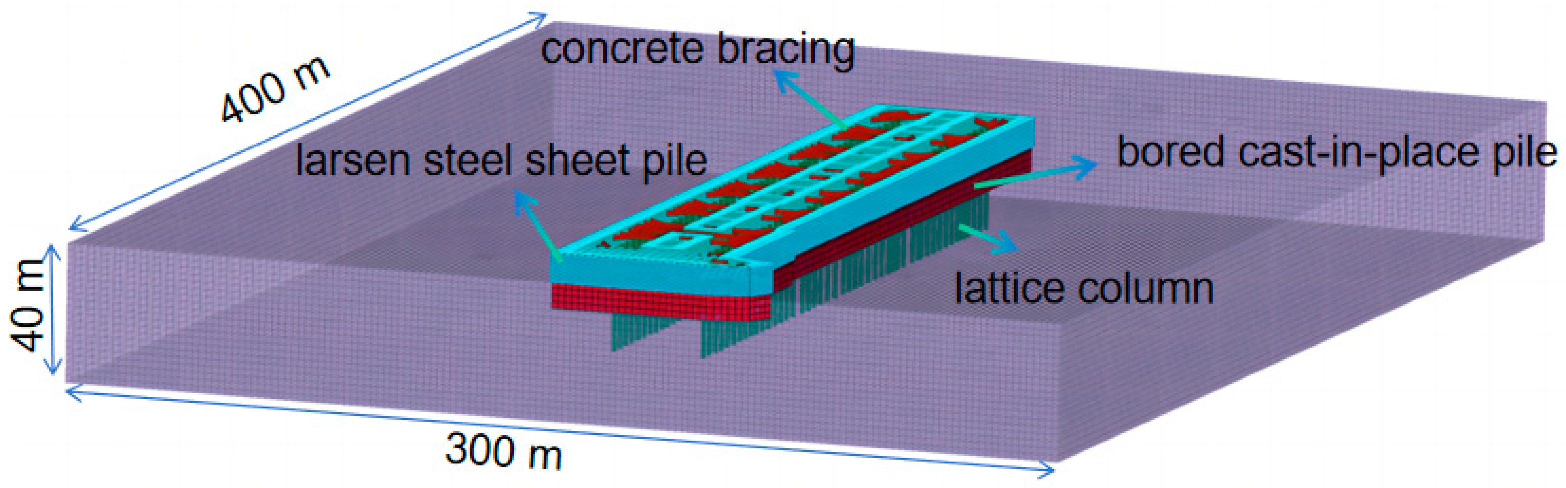
3.1. Computational Model

The computational model is detailed in Figure 1, and the layout plan of monitoring points is detailed in Figure 2. The model is numerically simulated using the finite difference method. In order to reduce the influence of size effects, the dimensions of the model were set at 300 m × 400 m × 40 m $(X\times Y\times Z)$ and the number of cells was 627,268. The $X$ and $Y$ axes are horizontal, and the $Z$ axis is vertical. The boundary constraints are normal constraints applied to the sides of the model, vertical constraints are applied to the bottom and the top surface is a free surface.

In order to avoid the influence of other factors in the process of pit excavation, the following assumptions were made during the numerical analysis process for the simulated construction process [33]:

• First, the soil in the stratum is continuously and horizontally distributed.
• Second, the soil is isotropic, its stress–strain varies in the Elasto-Plastic range and obeys the Mohr–Coulomb yield criterion.
• Third, only the self-weight of the soil is considered, not other loads during construction, and the final consolidation settlement of the soil is not considered. The numerical simulation was carried out using finite difference software (i.e., FLAC3D 6.0) for 3D modelling, with solid units for soil and bored cast-in-place pile, and PILE units for lattice columns and larsen steel sheet piles.

To simplify the calculations, the pit excavation was divided into four parts as shown in

Table 1. Construction Steps in the Numerical Model.

Construction Simulation Steps	Construction Description	Model Operation
1	Initial stress balance	Activate the silt layer and clay layer, set boundary conditions
2	Bored cast-in-place pile and enclosure construction	Activate structural unit (pile)
3	Excavation of the foundation pit of the bridge in the framework of Wenhua Road	Assign a 7 m empty model and excavate in two steps. The first step is to activate the beam unit, and the second step is to excavate to the bottom of the pit
4	Excavation of foundation pit for medium bridge bearing platform	Assign empty models to each bearing platform foundation pit to solve the balance

. Initial stress equilibrium is carried out in the first stage, and it is important to note that the ground stress initialization assumes that the soil in each layer is homogeneous, continuous and isotropic. The second stage assigns parameters corresponding to bored piles and lattice columns and larsen steel sheet piles, including PILE units. The third step is simulating the excavation of the Culture Road frames center bridge pit, and setting up monitoring points. The fourth step is simulating the excavation of the foundation pit of the bearing platform of the middle bridge.

3.2. Deterministic Analysis

When performing deterministic analyses, the model does not take into account the spatial variability of soil parameters. Soil parameters in the area were obtained through analysis of geological reports. The soil parameters were selected as shown in

Table 2. Physico-Mechanical Parameters in the Model.

Soil Type	Thickness (m)	Density (kg/m3)	Internal Friction Angle (°)	Cohesion (kPa)	Compression Modulus (MPa)
Clay ①1	2	1840	11.8	20.4	3.45
Mucky silty clay ②1	4	1800	15.6	8.7	3.22
Silt ③1	8	1620	9.0	9.7	1.63
Silt ③2	12	1630	13.7	9.3	1.78
Mucky silty clay ②2	14	1790	17.5	13.5	3.05

.

When the pit is excavated, the unloading of the soil causes the surrounding soil to move towards the excavation section, and concrete supports are set up to control the displacement of the pit wall to withstand the earth pressure and water pressure transferred from the enclosing wall. The concrete support is simulated using a beam unit and the axial force cloud at different construction stages is shown in Figure 3.

Excavation of the pit leads to compression of the surrounding soil into the pit and thus the pressure on the support. Figure 3 shows that when the pit is excavated at different stages, the maximum axial force of the support is 3.8 × 10⁵ N, 1.9 × 10⁶ N and 2.8 × 10⁶ N, respectively, which is distributed in the middle of the pair of support trusses near the minimum axial force of the pair of support trusses, which is 2.8 × 10⁵ N, 1.7 × 10⁶ N and 1.7 × 10⁶ N. The distribution of axial force is characterized by the two sides being small, the middle is large and the axial force is increased close to the heteromorphic region. Therefore, the central buttress truss, as a vulnerable area of the supporting structure, should be strengthened for emphasis on reinforcement and subsequent monitoring.

The depth of excavation resulted in an inconsistent performance of horizontal deformation of the bored cast-in-place piles: the value of horizontal displacement decreases with increasing depth when the excavation depth is small, and increases with increasing depth after the excavation is completed. In addition, the slope of the displacement curve in Figure 4c is greater than that in Figure 4a,b, and the rate of change of the retaining wall displacement increases simply due to the release of more stresses from the excavation. This is the “depth effect” of pit excavation, as the excavation of shallow soil layers in a pit can generate more stresses than the excavation of deeper soil layers in a pit.

As shown in Figure 5a, the vertical displacement curve of the top of the bored cast-in-place piles has three main parts. During the initial excavation, the settlement of the enclosing pile is small due to the shallow depth of excavation and the small amount of soil unloading. Continuing excavation to the bottom of the pit, the settlement of the enclosing piles increased steadily, settlement values of 4 mm and 6 mm on both sides, before stabilizing. In addition, there is a significant difference in the settlement values between z1 and z10 and z11 and z12. The settlement value of 6–8.3 mm at monitoring points z1–z10 is greater than that of 3–4 mm at monitoring points z11–z20, and the settlement value is less than the prescribed warning value of 20 mm. The reason for asymmetric settlement may be due to the following reasons: (1) The foundation pit of the pier cap is located near the monitoring points z1–z10, and the excavation of the foundation pit of the pier cap causes significant soil unloading in this direction, resulting in significant settlement of the retaining piles. (2) The asymmetric arrangement of three-axis cement mixing piles in the foundation pit causes uneven settlement. (3) Due to approximating the retaining pile as an underground continuous wall in the numerical simulation and assuming good integrity, the settlement at z1–z10 causes a slight uplift at z11–z20, resulting in asymmetric settlement values due to the coupling of various reasons.

As shown in Figure 5b, the top of the bored cast-in-place piles were slowly displaced into the pit during the first step of pit excavation for the erection of concrete support, with a displacement of 0.5 mm, further excavation at this point showed almost linear growth in displacement, and the displacement at each monitoring point was in the range of 1.5–2.0 mm, and reached a peak with the excavation of the bearing platform pit, which further grew to 2.8 mm. When the excavation of the foundation pit causes the soil in this area to unload, the three-axis cement mixing piles outside the foundation pit of each foundation pit generate horizontal displacement towards the pit under the active soil pressure of the surrounding soil, forming a “lever” with a certain point as the fulcrum, which causes the soil outside the pit to bulge and increases the passive soil pressure of the retaining piles, offsetting some of the displacement towards the pit. This causes the soil outside the pit to protrude, and the horizontal displacement rebounds towards the outside of the pit, stabilizing to a position of 1.5–2.5 mm. This is also reflected in reference [34].

As shown in Figure 6, the monitoring data of the corresponding points are well connected with the simulation data, so the selected parameters of numerical simulation basically meet the requirements, which can be used as a basic model for the study of the effect of considering the spatial variability of soil parameters on the stability of the excavation of the super-large foundation pit. However, the results of the numerical simulation are relatively large monitoring data, which is due to the numerical simulation itself and the limitations of the structure in the software.

3.3. Stochastic Analysis

Uncertainty includes various representative values of action, properties and parameters of materials, reliability and accuracy of design, calculation and construction, as well as meeting economic, political, social and environmental requirements. Compared to the uncertainty of engineering materials and loads, the spatial variability of the mechanical parameters of soil has a more important impact on engineering construction due to non-artificial reasons [35,36,37].

In order to study the effect of spatial variability of geological parameters on the stability of excavation of super-large foundation pits, and to show the research results more intuitively, this section starts from the comparison with the research content in Section 3.2. The following assumptions are made to ensure the accuracy and conciseness of the study: (1) The uncertainties of the remaining parameters are not taken into consideration at this time. (2) The soil shear strength index values ($c, \phi$) are random fields that follow a log-normal distribution. (3) The soil body is isotropic, meaning that the correlation distances between the horizontal and vertical directions are equal. (4) The parameters of the various soil layers are independent of one another.

The finite difference method and the theory of random fields are used to do the stochastic analysis. To study the coefficient of variation and the impact of the soil cohesion $c$ value and the friction coefficient $\phi$ value on the ground surface deformation pattern in an isotropic random field ($\theta =\theta x=\theta z$), the coefficient of variation $\lambda$ and the mean value $\mu$ are taken as indicated in

Table 3. Random Coefficients of Each Soil Layer.

Soil Type	Cohesion (kPa)		Internal Friction Angle (°)
	Mean Value μc	CV λc	$\mathbf{Mean} \mathbf{Value} {\mathsf{\mu }}_{\mathsf{\phi }}$	$\mathbf{CV} {\mathsf{\lambda }}_{\mathit{\phi }}$
Clay ①1	20.4	0.198	11.8	0.136
Mucky silty clay ②1	8.7	0.265	15.6	0.188
Silt ③1	9.7	0.075	9.0	0.088
Silt ③2	9.3	0.047	13.7	0.131
Mucky silty clay ②2	13.5	0.181	17.5	0.187

.

Using random field theory, the Wenhua Road hole was numerically simulated. The concrete support was likewise simulated using a beam unit, and the resulting cloud diagram of the axial force distribution of the concrete support is displayed in Figure 7.

To determine the influence of various procedures on the final findings, two methods—uniform and gaussian—are utilized to produce the stochastic parameters. With the exception of a gap in the axial force values at each stage, the distribution of the support axial force obtained after taking the geologic parameters’ spatial variability into account is similar to that in Figure 3 without taking the geologic parameters’ spatial variability into account, which is small on both sides and large in the middle. The primary cause of the discrepancy is the various stochastic methods used to assign the soil parameters. The uniform distribution method, which is a simpler stochastic model, generates a random field with the same probability for all values and no obvious peaks or tails, whereas the Gaussian distribution method, which is a stochastic model based on the normal distribution, is more appropriate given the regular distribution of the geotechnical body parameters because its shape is determined by the mean and standard deviation. The Gaussian distribution approach is comparatively more applicable as compared to the regular distribution of geotechnical parameters.

Combining the parameters from Table 2 and Table 3 allows the programming language to write the “Generate Random Field” code, which is then run to obtain the random field database taking spatial variables into consideration. Then, after post-processing, the influence of the coefficient of variation on the settlement and horizontal displacement of the soil surrounding the pit excavation and the settlement and horizontal displacement of the enclosing piles for any 50 calculations is obtained; the results of the calculations are displayed in Figure 8 and Figure 9.

It can be seen that when the ground investigation report’s coefficient of variation and the mean values of cohesion and angle of internal friction are used to create a random field for the simulation, the results of the stochastic analysis fluctuate up and down, but the curves’ shapes remain unchanged. This suggests that the coefficient of variation primarily affects the quantitative value of surface deformation and the deformation of enclosing piles, with little to no impact on the deformation’s shape. The conclusion drawn is similar to the research results of other scholars on tunnel excavation and foundation pit excavation [38,39,40]. In addition, as recorded in the literature, the ground settlement obtained by comparing deterministic analysis with random analysis is larger. As shown in Figure 8, compared with the deterministic results, it is shown that the soil has a weakening effect after considering spatiality and disturbance. The maximum settlement of the soil layer around the foundation pit increases by 1.5 mm, and the horizontal displacement increases by 4 mm. For retaining piles, due to the fact that the soil is considered as a whole in deterministic analysis, the material parameters of each point inside the soil are the same. In random analysis, there may be large areas of low stiffness within the soil. This resulted in significant displacement of the retaining piles under random analysis. The maximum horizontal displacement of the retaining pile is greater than 1.5 mm, and the vertical displacement reaches 1.0 mm.

More obviously, the deformation region is smaller and less symmetrically distributed when taking into account the spatial variation of the geologic parameters than when the spatial variability is not taken into account. This is because each unit soil parameter has a stochastic nature, exhibiting different properties within the soil representation function and mapping these properties to the unit. This is in contrast to the deterministic analysis. Under this random condition, it exhibits overall asymmetry in the raised region. At the same time, the deformation curve exhibits a certain degree of discreteness during the randomness analysis, which is more in line with the large variability and high complexity of rock and soil properties compared to the results obtained from the deterministic analysis. Therefore, using random models for a geotechnical engineering construction simulation has a more accurate prediction.

Therefore, when carrying out the construction of super large and irregular foundation pits, attention should be paid to strengthening the areas that are prone to deformation, in order to reduce the deformation of the retaining structure during excavation and ensure construction safety and quality. This is of great significance for shortening the construction period, saving costs and ensuring construction safety.

4. Conclusions

• The effect of spatial variability of soil parameters can be effectively included in the study of envelope displacement and surface deformation problems resulting from foundation excavation construction when random field theory and numerical analysis are combined.
• Merely studying the mean function and correlation function of a random field cannot replace studying the entire random field, but they do describe the main statistical characteristics of the random field. Therefore, they often play an important role in solving practical engineering problems. The essence of random field theory is to use homogeneous normal distribution random fields to simulate the spatial distribution of geotechnical parameters, and to characterize the spatial variability and correlation of geotechnical parameters using variance, correlation function and correlation distance.
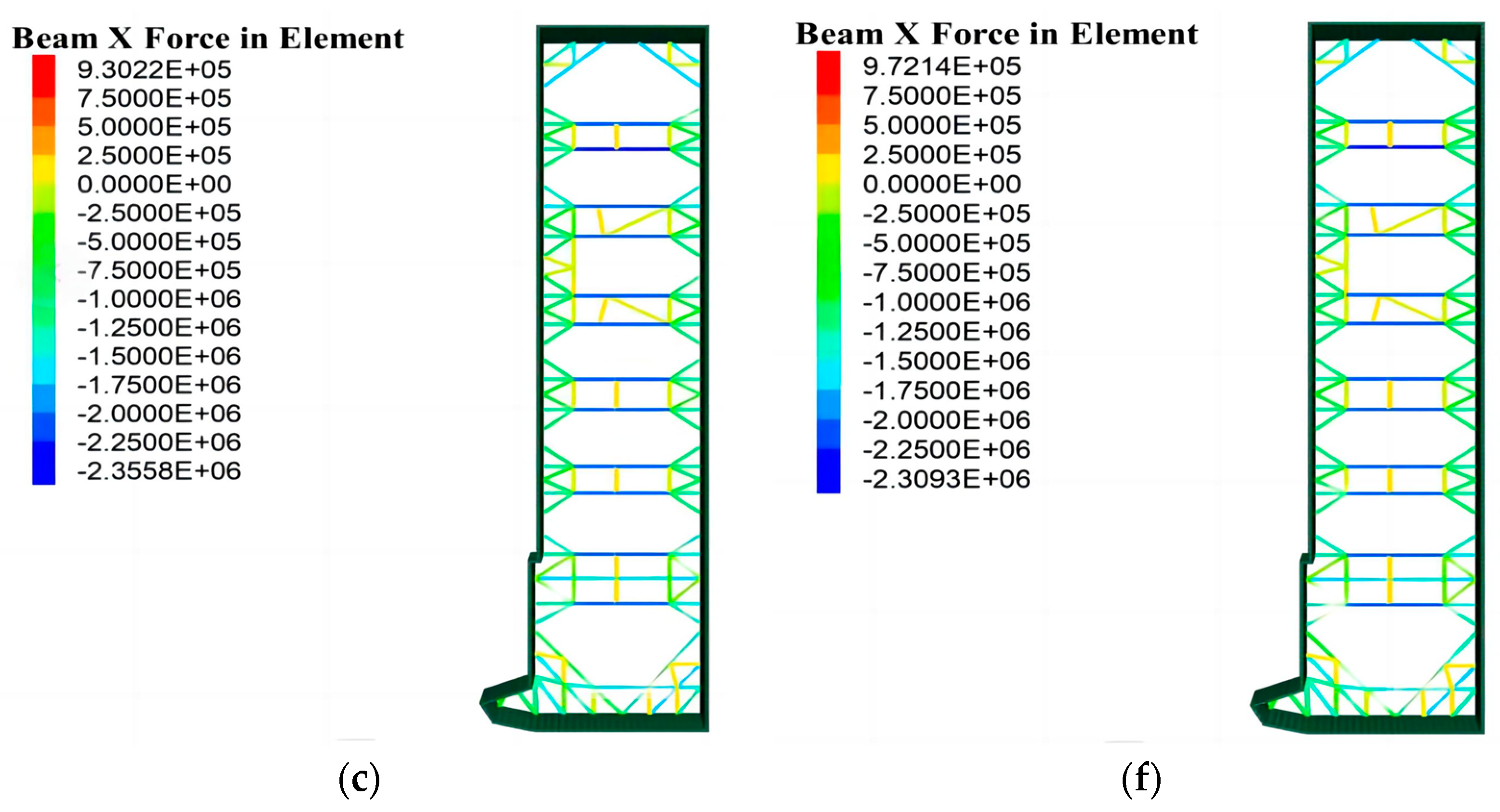
• The maximum axial force of the pit excavation support is distributed in the center of the buttress truss, while the minimum axial force of the buttress truss mainly occurs in the two sides, the overall distribution of the axial force is small in the two sides and large in the middle and the axial force is larger near the shaped area.
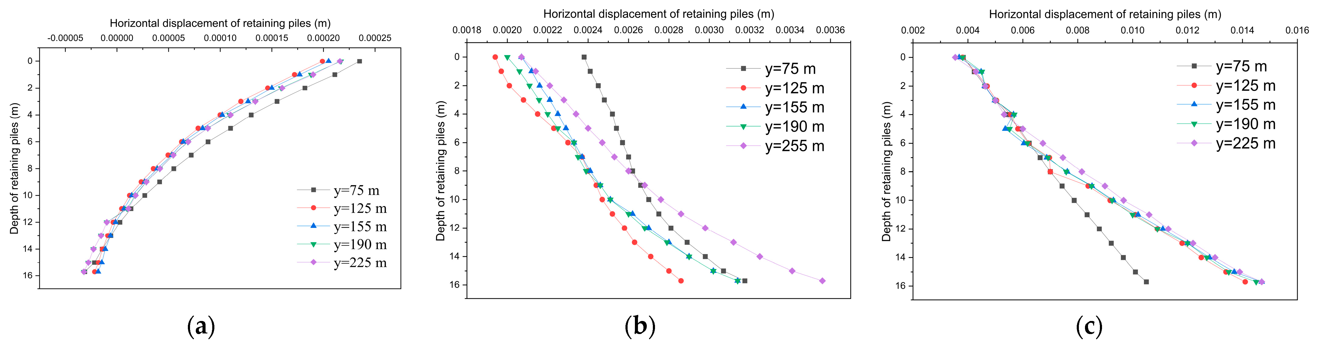
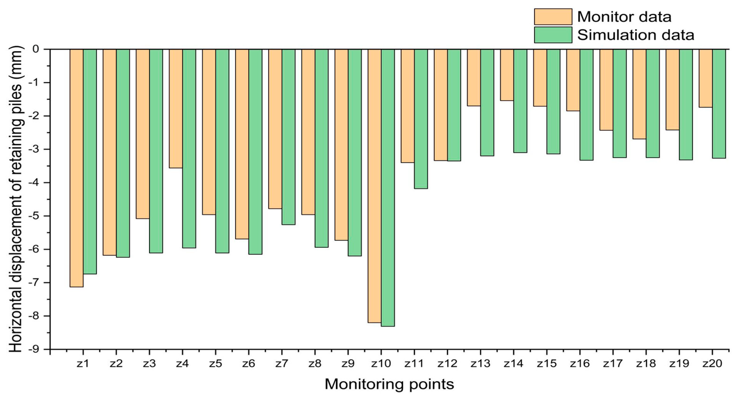
• The reason for the perimeter piles’ tendency to partially rebound out of the pit during the excavation of the bearing platform foundation pit is that, as a result of the soil being unloaded during the excavation process, the triaxial piles mixed with cement outside the bearing platform foundation pit were displaced horizontally to the pit under the active soil pressure of the surrounding soil, forming a “lever” with a specific point serving as a pivot point. This caused the soil outside the pit to bulge, which increased the perimeter piles’ passive soil pressure and partially offset some of the displacements into the pit.
• A uniform distribution and a Gaussian distribution are used to examine the impact of the shear index’s geographic variability on the stability of the foundation pit, provided that an appropriate shear strength index is chosen. By comparison of the soil layer displacement analysis, bored cast-in-place piles displacement analysis and support force analysis by taking spatial variability into account or not, it is discovered that doing so has no discernible effect on the shape of each curve; nonetheless, taking spatial variability into account results in a big displacement value and a tiny support axial force value.
• After taking into account the spatial variability, the soil layer may not deform symmetrically, and the soil will be more affected by the pit excavation in the area of low stiffness.

References

1. Guo, P.; Gong, X.; Wang, Y.; Lin, H.; Zhao, Y. Analysis of observed performance of a deep excavation straddled by shallowly buried pressurized pipelines and underneath traversed by planned tunnels. Tunn. Undergr. Space Technol. 2023, 132, 104946. [Google Scholar] [CrossRef]
2. Li, J.J.; Li, M.G.; Chen, H.B.; Chen, J.J. Numerical investigation of the effects of compressibility of gassy groundwater (CGG) on the performance of deep excavations in Shanghai soft deposits. Eng. Geol. 2023, 327, 107306. [Google Scholar] [CrossRef]
3. Li, P.F.; Li, Z.; Ge, C.H.; Guo, F. Deformation characteristics and redundancy analysis of deep foundation pit excavation in sandy soil cover excavation reverse construction subway station. Tunn. Constr. 2023, 43, 98–108. [Google Scholar]
4. Kog, Y.C. Deep Excavation in Soft Normally Consolidated Clay. Pract. Period. Struct. Des. Constr. 2023, 28, 04023001. [Google Scholar] [CrossRef]
5. Tu, B.; Zheng, J.; Ye, S.; Shen, M. Study on Excavation Response of Deep Foundation Pit Supported by SMW Piles Combined with Internal Support in Soft Soil Area. Water 2023, 15, 3430. [Google Scholar] [CrossRef]
6. Wang, D.; Ye, S.; Xin, L. Study on the Analysis of Pile Foundation Deformation and Control Methods during the Excavation of Deep and Thick Sludge Pits. Water 2023, 15, 3121. [Google Scholar] [CrossRef]
7. Wu, G.Q.; Nie, J.G. Reliability analysis of karst foundation considering spatial variability of strata. J. Hunan Univ. 2022, 49, 45–53. [Google Scholar]
8. Wu, Y.X.; Zhou, X.H.; Gao, Y.F.; Zhang, L.; Yang, J. Effect of soil variability on bearing capacity accounting for non-stationary characteristics of undrained shear strength. Comput. Geotech. 2019, 110, 199–210. [Google Scholar] [CrossRef]
9. Gan, X.L.; Gong, X.N.; Liu, N.W.; Yu, J.L.; Li, W.B. Random analysis method for nonlinear interaction between shield tunnel and spatially variable soil. Comput. Geotech. 2023, 166, 105964. [Google Scholar] [CrossRef]
10. Lumb, P. The variability of natural soils. Can. Geotech. J. 2011, 3, 74–97. [Google Scholar] [CrossRef]
11. Vanmarcke, E.H. Probabilistic modeling of soil profiles. J. Geotech. Eng. Div. 1977, 103, 1227–1246. [Google Scholar] [CrossRef]
12. Vanmarcke, E.H. Random Fields: Analysis and Synthesis; MIT Press: Cambridge, MA, USA, 1983; pp. 1–382. [Google Scholar]
13. Zhang, J.Z.; Wang, H.J.; Liu, F.S. Computer simulation and engineering application of soil-parameter random field in geotechnical engineering. J. Water Resour. Arch. Eng. 2017, 15, 8–13. [Google Scholar]
14. Jiang, X.; Xiao, Y.; Zhou, X.D.; Zhao, X.D. The application of random field theory in reliability evaluation of vacuum preloaded soft soil foundation. Soil Eng. Found. 2022, 36, 230–234. [Google Scholar]
15. Cheng, H.Z.; Chen, J.; Li, J.B. Study on surface deformation induced by shield tunneling based on random field theory. J. Rock Mech. Eng. 2016, 35, 4256–4264. [Google Scholar]
16. Zhang, X.Y.; Shi, C.H.; Sun, X.H.; Peng, L.M.; Zheng, K.Y. Analysis of Surface Deformation Characteristics during Pipe Jacking Tunnel Construction Based on Random Field Theory. J. Cen. South Univ. 2023, 54, 2174–2189. [Google Scholar]
17. Gan, X.L.; Yu, J.L.; Bezuijen, A.; Gong, X.N.; Wang, C.C. Tunneling-induced longitudinal responses of existing tunnel with discontinuities in structure stiffness. Transp. Geotech. 2023, 42, 101113. [Google Scholar] [CrossRef]
18. Zheng, J.J.; Qiao, Y.Q.; Zhang, R.J. Effect of spatial variability of engineering properties on holistic performance of passive zone improvement for deep excavation in soft soil. J. Civil Environ. Eng. 2019, 41, 1–8. [Google Scholar]
19. Wen, G.; Wang, Q.; Chen, F.y. Reliability analysis of slopes considering spatial variability of rock mass and random response study of anti slip piles. Rock Soil Mech. 2021, 42, 3157–3168. [Google Scholar]
20. Cheng, Y.G.; Chang, X.L.; Li, D.Q. Deformation stochastic analysis of tunnel surrounding rock considering its spatial randomness. J. Rock Mech. Eng. 2012, 31, 2767–2775. [Google Scholar]
21. Cheng, H.Z.; Chen, J.; Hu, Z.F. Evaluation of safety of buildings above tunnels accounting for spatial variability of soil properties. J. Geotech. Eng. 2017, 39, 75–78. [Google Scholar]
22. Seyedpour, S.M.; Henning, C.; Kirmizakis, P.; Herbrandt, S.; Ickstadt, K.; Doherty, R.; Ricken, T. Uncertainty with Varying Subsurface Permeabilities Reduced Using Coupled Random Field and Extended Theory of Porous Media Contaminant Transport Models. Water 2023, 15, 159. [Google Scholar] [CrossRef]
23. Lu, H.; Li, H.; Meng, X. Spatial Variability of the Mechanical Parameters of High-Water-Content Soil Based on a Dual-Bridge CPT Test. Water 2022, 14, 343. [Google Scholar] [CrossRef]
24. Hwang, J.; Lee, H.; Lee, K. Effects of Nonhomogeneous Soil Characteristics on the Hydrologic Response: A Case Study. Water 2020, 12, 2416. [Google Scholar] [CrossRef]
25. Wang, G. Analysis of Slope Reliability Simulation Based on Covariance Decomposition Method. Rural Econ. Sci. Tech. 2020, 31, 67–69. [Google Scholar]
26. Liu, B.C.; Bao, H.; Yao, F.Z. Analysis of the impact of tunnel excavation on uneven settlement and surface deformation of nearby buildings based on random field theory. Henan Sci. 2020, 38, 1258–1263. [Google Scholar]
27. Wang, J.W.; Zhou, S.; Chen, F. Calculation and analysis of soil properties related distance of soft clay in Ningbo. Yangtze River 2020, 51, 208–212+220. [Google Scholar]
28. Yan, S.W.; Zhu, H.X.; Liu, R. Study on application of random field theory to reliability analysis. J. Geotech. Eng. 2006, 12, 2053–2059. [Google Scholar]
29. Gui, Z.P. Practical Evaluation Method for Deformation of Deep Foundation Pits in Soft Soil Considering Soil Properties and Randomness of Construction Parameters. Ph.D. Thesis, Huazhong University of Science and Technology, Wuhan, China, 2020. [Google Scholar]
30. Wang, M.X.; Wu, Q.; Li, D.Q.; Du, W.Q. Numerical-based seismic displacement hazard analysis for earth slopes considering spatially variable soils. Soil Dyn. Earth. Eng. 2023, 171, 107967. [Google Scholar] [CrossRef]
31. Zhang, P.S.; Shi, J.Y. Analysis of effects of space variability of parameters on soil deformation around the deep exception. J. Under. Space Eng. 2008, 1, 111–115+137. [Google Scholar]
32. Wang, Z.S.; Chen, J.; Rong, H. Characterization and modeling methods for anisotropic random fields of soil parameters. J. Comput. Mech. 2021, 38, 29–36. [Google Scholar]
33. Wei, Y.J.; Niu, G.; Dong, J.K. Research on the Engineering Application of Artificial Freezing Method in Shield Tunneling Reception in Soft and Rich Water Strata. Eng. Constr. 2021, 35, 819–823. [Google Scholar]
34. Wang, Y.; Chen, S.; Ouyang, J.; Li, J.; Zhao, Y.; Lin, H.; Guo, P. Predicting Ground Surface Settlements Induced by Deep Excavation under Embankment Surcharge Load in Flood Detention Zone. Water 2022, 14, 3868. [Google Scholar] [CrossRef]
35. Ren, D.W.; Zeng, L.L.; Zhang, H.; Li, C.T. Applicability study of equivalent models for spatial variability of geotechnical parameters. J. Wuhan Univ. Technol. 2023, 47, 540–544. [Google Scholar]
36. Liu, Z.; He, P.; Zhang, A.Q. Research on the Influence of Soil Mechanics Parameters on Stratum Disturbance with Dynamic Changes of Tunnel Construction. Mod. Tunn. Technol. 2017, 54, 131–136. [Google Scholar]
37. Feng, Z.J.; Li, D.; Jiang, G. Stability analysis of secondary excavation of high slopes based on reliability theory. Sci. Technol. 2023, 19, 130–136. [Google Scholar]
38. Zhang, L.S.; Li, D.Q.; Cao, Z.J.; Tang, X.S. Efficient Monte Carlo analysis method for reliability of foundation pit deformation considering statistical uncertainty. J. Wuhan Univ. 2019, 52, 207–215. [Google Scholar]
39. Yan, L.; Wang, Q.; Liu, L.J. Reliability analysis of soil slopes based on random field theory. Water Conser. Sci. Econ. 2023, 29, 13–16+28. [Google Scholar]
40. Wu, G.F.; Chen, C.; Wang, X. Slope stability analysis based on random field theory and strength reduction method. Eng. Constr. Stand. 2021, S1, 111–115. [Google Scholar]
Figure 1. 3D Model of Foundation Pit Retaining Structure.
Water 16 00098 g001
Figure 2. Layout Plan of Monitoring Points. Where z1–z20 are vertical displacement monitoring points for the retaining piles.
Water 16 00098 g002
Figure 3. Cloud Chart of Concrete Support Axial Force at Each Construction Stage: (a) step 1; (b) step 2; (c) step 3.
Water 16 00098 g003
Figure 4. Horizontal Displacement Curve of Bored Cast-in-Place Piles at Different Cross-sections at x = 130 m: (a) step 1; (b) step 2; (c) step 3.
Water 16 00098 g004
Figure 5. Deformation Diagram of the Top of the Bored Cast-in-Place Piles. (a) Vertical Displacement Diagram of the Top of the Bored Cast-in-Place Piles, (b) Horizontal Displacement Diagram of the Top of the Bored Cast-in-Place Piles.
Water 16 00098 g005
Figure 6. Comparison of Vertical Displacement at the Top of the Bored Cast-in-Place Piles.
Water 16 00098 g006
Figure 7. Cloud Chart of Concrete Support Axial Force at Each Construction Stage of Random Field Model: (a) uniform-step1; (b) uniform-step2; (c) uniform-step3; (d) gaussian-step1; (e) gaussian-step2; (f) gaussian-step3.
Water 16 00098 g007aWater 16 00098 g007b
Figure 8. Curve of the Influence of Variation Coefficient on Ground Displacement for Any 50 Calculations. (a) Ground Settlement Curve at Different Positions from the Center of the Foundation Pit; (b) Horizontal Displacement Curve of the Ground at Different Positions from the Center of the Foundation Pit.
Water 16 00098 g008
Figure 9. Curve of the Influence of Variation Coefficient on the Displacement of Bored Cast-in-Place Piles After Any 50 Calculations. (a) Vertical Displacement Curve of Bored Cast-in-Place Piles at Different Positions from the Center of the Foundation Pit; (b) Horizontal Displacement Curve of Bored Cast-in-Place Piles at Different Positions from the Center of the Foundation Pit.
Water 16 00098 g009