Abstract
DO is an important index to characterize environmental water quality. The time series fluctuation of DO can be analyzed via frequency band decomposition, which is very valuable for water quality simulations. In this paper, DO in the Chengdu area of China was studied using variational mode decomposition with daily meteorological data and water quality data from 2020 to 2022. After variable decomposition, the DO data were first decomposed into different frequency band signals named IMF1, IMF2, IMF3, IMF4, and IMF5. IMF1 represented the low-frequency signal with long-term trend characteristics of the data. IMF2 to IMF5 represented the high-frequency signal with short-term mutation characteristics of the data. By combining the variable decomposition results with the correlation analysis, it was found that the long-term trend characteristics of DO are affected by the superposition of meteorological factors, hydrological factors, and water pollution factors but have a weak correlation with any single determining factor. The air temperature, water temperature, phosphorus, air pressure, pH value, chemical oxygen demand, and nitrogen were relatively strongly correlated with the long-term trend characteristics of DO. The short-term mutation characteristics of DO were mainly determined using the characteristics of the water body itself, while the influence of the meteorological factors could basically be ignored. The water temperature, pH value, and eutrophication were the biggest influencing factors. Then, a predictive framework combining frequency division with a deep learning model or a machine learning model was constructed to predict DO. The predicted results of GRU, random forest, and XGBoost with and without the framework were compared. It was shown that, after removing the interference factors with correlations less than 0.3, the predicted value of DO was much closer to the actual value. The XGBoost and random forest models with decomposed signals had a high degree of simulation fitting and could be used to predict DO in the Chengdu area. The above research approach can be applied to further explore the prediction of various pollution factors in different areas of China.
1. Introduction
Dissolved oxygen (DO) is an important index to characterize environmental water quality and is affected by complex, dynamic, and non-linear factors. As one of the critical elements of the aquatic environment, DO can control the survival of aquatic organisms, the decomposition type of organic pollutants, and the strength of the self-purification of water bodies. An anoxic environment will further lead to the release of nitrogen, phosphorus, and other pollutants from the sediment into the water, which will adversely deteriorate the water quality [1,2,3]. Changes in the dissolved oxygen content in intensive aquaculture ponds are influenced by meteorological data and other water quality parameters [4,5]. The temperature, body mass, mineralization of organic matter, and several environmental factors, such as solar irradiance, water temperature, pH, turbidity, rainfall, and wind speed, also affect the dynamics of DO [6]. The physical and chemical factors that influence the level of DO in water also include water surface agitation and chemical oxygen consumption, such as sulfide oxidation and nitrification. The biological factors are photosynthesis and aerobic respiration. The significant discharge of nutrients in an aquatic system can decrease the DO concentration because of the relevant biological and chemical impacts [7,8].
Due to the non-linear and complex changes in DO data, it is very important to predict and simulate the dissolved oxygen content and process changes for water environment health assessment and management. Various numerical models have been established by scholars all over the world to study the time series fluctuation of DO. A dynamic model of a dissolved oxygen complex with the help of a single dimension differential equation was proposed, in which the dynamics of DO in relation to the nature of the solar irradiance, temperature, salinity, and mineralization of particulate organic matter were studied as well as the influence of reaeration and wind velocity on estuarine DO dynamics [9]. A dynamic DO model was developed using STELLA to predict the variations of the net ecosystem metabolism (NEM) in the Yellow River Estuary, in which the simulation error was kept under 23%. Via the sensitive analysis of the model, the temperature was found to be the most remarkable factor affecting the metabolic rates at individual sites [10]. A numerical simulation of DO concentrations was discussed using the TELEMAC-WAQTEL-O2 model, which was applied to investigate the effect of different weather conditions, including the tide, mean and maximum wind, and different water temperatures, on DO in Egypt [11]. A process-based model chain (the lake model PROTECH drived by the INCA-N and INCA-P catchment models) was used to quantify the effectiveness of terrestrial nutrient control measures on DO concentrations. Nutrient load reductions were a significant driver of increased DO concentrations, associated with changes in the water temperature and chemistry [12]. As a multi-factor hydrological process simulation model, including a quantitative numerical simulation technique, the water assessment tool (SWAT) model was developed and is often used to simulate and predict hydrological processes. The numerical simulation of non-point source pollution can also be realized using the SWAT model [13]. However, an obvious shortcoming of this model is that it needs to collect a large amount of information, such as the hydrology, meteorology, geology, land use, farming methods, crop types, and regional economy as the input parameters, which makes the model calibration and construction complicated [14].
In order to solve the inconvenience caused by the lack of data in numerical models, machine learning models were applied to attempt to simulate and predict water quality [15]. Machine learning techniques constituted by a set of algorithms and statistical models are widely used in water quality monitoring and prediction [16,17]. Machine learning techniques can enhance predictive capabilities by considering non-linear interactions and capturing underlying complexities, particularly ANNs (artificial neural networks). The ANN model, equipped with the Levenberg–Marquardt algorithm, which is effective in training and optimizing network parameters, can effectively capture complex relationships and provide reliable DO predictions [18]. Two ANN models, the feed-forward neural network (FFNN) and radial basis function neural network (RBFNN), were developed to predict the dissolved oxygen from the biochemical oxygen demand (BOD) and chemical oxygen demand (COD) in the Surma River, which indicated that the ANN model could be employed successfully in estimating the dissolved oxygen in the Surma River [19]. Another machine learning method, the support vector machine (SVM), was also applied in water environment assessments and was thought to be better than the ANN because the SVM can deal with non-linear problems when identifying some predictive solutions [20,21]. A predictive modeling framework based on support vector regression (SVR) was proposed to analyze and predict the spatiotemporal variations of the DO concentration in this world-renowned mega project, which could also identify and reveal the key parameters that should be concerned and monitored under different environmental factor changes [22]. As a classical neural network model, the backpropagation neural network (BPNN) model has the ability to extract non-linear relationships from the input factors with high interpretability while its local convergence can be avoided. It is a multi-layer feed-forward network trained according to an error backpropagation algorithm, which usually contains an input layer, an output layer, and one or more hidden layers [23]. A unique AEABC-BPNN model was carried out through the non-linear input and output fitting function of the BPNN model, which has the dual advantage of self-renewal and global iterative updates under the effect of the adaptive evolution strategy [24]. A novel clustering-based soft plus extreme learning machine method (CSELM) was provided to predict dissolved oxygen changes accurately and efficiently from time series data, which achieved better prediction results than other models in terms of accuracy and efficiency in a real-world dissolved oxygen content prediction [4].
Deep learning models have the characteristics of multi-layer feedback simulations, which can overcome the critical time limitation of machine learning models. In recent years, research into deep learning models in water quality analyses and predictions has been paid more and more attention. The recurrent neural network (RNN) is a recursive neural network algorithm that can learn the non-linear features of sequence data to realize time series predictions [25]. The long and short-term memory network (LSTM) model, as a typical deep learning model, is particularly adaptable to time series predictions due to its high accuracy and good scalability, which can solve the problem of long delays and long interval time series [26]. A LSTM model combining the gradient boosting decision tree (GBDT) was proposed to select the characteristic factors with a strong influence on DO in the standard pond of the Jintan fishery base in China [27]. A gated recurrent unit (GRU) based on LSTM optimizes the LSTM network structure while maintaining LSTM performance [28]. With a fixed number of parameters, a GRU has advantages in the convergence of CPU time, parameter updates, and generalization over LSTM [29]. The long-term learning dependence of a GRU can capture the long-term correlation of water quality data and realize the periodic rule of water quality data for a long period, which can predict the water quality accurately by reflecting the continuous water pollution process. The GRU model was verified to be better than some linear models, such as the autoregressive integrated moving average (ARIMA) model [30]. A PCA-PFA-GRU model was established to predict the dissolved oxygen in perch culture water quality, in which a principal component analysis (PCA) was used to eliminate the redundant variables and reduce the data dimension and complexity first. The dissolved oxygen, water temperature, and conductivity were chosen to substitute for the original variables [31].
As a time-frequency domain transformation method, variational mode decomposition (VMD) can reduce the non-stationarity of time series with high complexity and strong non-linearity and obtain relatively stable subsequences containing multiple different frequency scales. It is an adaptive and completely non-recursive variational and signal mode processing method proposed in 2014 [32]. It has the advantage of determining the number of mode decompositions. Its adaptability is manifested in determining the number of mode decompositions of a specific sequence according to the actual situation, and then the center frequency and finite bandwidth of each mode can be adaptively matched in the subsequent search and solution process. In this way, the effective separation of the intrinsic mode function (IMF) and the frequency domain division of the signal can be realized to obtain the effective decomposition components of the signal provided and finally obtain the optimal solution to the variational problem. The VMD method overcomes the problems of the end effect and aliasing of the modal components in the empirical mode decomposition (EMD) method, which avoids the aliasing phenomenon by controlling the bandwidth so as to be suitable for non-stationarity sequences.
According to the characteristics and advantages of frequency division, it can be speculated that the interpretability and accuracy of the model will be improved by using the VMD method to decompose and screen the factors affecting water quality first and then conducting a model simulation. There are few reports on the construction of a predictive framework by combining frequency division with a machine learning model or deep learning model in non-point source pollution research. Taking DO as the main research index and six rivers in the Chengdu area as the research object, the influencing factors of water quality in the Chengdu area were attempted to be decomposed and screened by using the VMD method in this paper. After that, the GRU, random forest, and extreme gradient boosting (XGBoost) were used to predict DO before and after variational mode decomposition in order to compare the effects of variational mode decomposition on the prediction of DO in practice. The new prediction framework combining VMD with an intelligent model to simulate DO is hoped to improve the simulation accuracy and contribute to water area management.
2. Methodology
2.1. Study Area
The water system of Chengdu is mainly composed of the Minjiang River basin and the Tuojiang River basin. The water system of Chengdu is shown in Figure 1. In recent years, Chengdu has vigorously carried out urban ecological construction, such as increasing the area of wetlands, extending the green area, and strengthening the control of urban non-point source pollution. These measures have greatly improved the water environment quality of Chengdu’s water systems, but there are still many water systems that cannot meet or even exceed the environmental quality standards for surface water in China. The research on the water pollution factors of these substandard water systems must be more and more detailed and improved so as to meet the requirements of water pollution control and water area management in this area and, finally, to truly meet the needs of urban development in the Chengdu area.
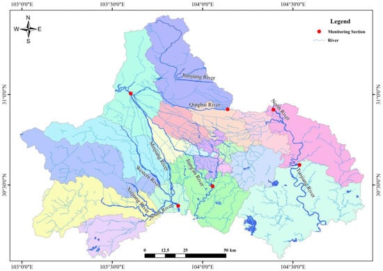
Figure 1.
The water system of Chengdu City.
2.2. Variational Mode Decomposition (VMD)
According to Konstantin Dragomiretskiy [32], VMD can obtain all the modes of signal decomposition through iterative updating and can divide the original data into signals of multiple frequency bands. The low-frequency signal represents the long-term trend characteristics of the original data, and the high-frequency band represents the short-term mutation characteristics. It minimizes the sum of the modal components to make the signal separation more thorough. Compared with empirical mode decomposition, it has better anti-noise ability and can overcome the problem of mode aliasing. Its constraint model can be expressed as the following equation:
where and are shorthand notations for the set of all modes and their center frequencies, respectively. Equally, is understood as the summation of all the modes. Then, a Lagrangian augmentation term is constructed to remove the constraints in (1) as follows:
The solution to the original minimization problem (1) was found as the saddle point of the augmented Lagrangian in a sequence of iterative sub-optimizations called the alternate direction method of multipliers (ADMMs) (see Algorithm 1). The ADMMs allows for the complete optimization problem to be broken down into a series of iterative sub-optimization problems. The iterative steps are as follows:
| Algorithm 1: ADMM optimization concept for VMD |
The model forecasting framework is shown in Figure 2. First, the raw data are decomposed into more regular signals of different frequency bands using VMD. Secondly, a filter is used to remove the signals that are weakly related to the predicted target. Then, the signal is sent to the model. By learning the change law of the data, the evolution process is simulated, and the future change is predicted. Finally, the prediction results are obtained by summing the different signal values predicted using each model.
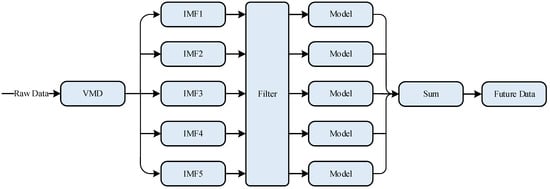
Figure 2.
Model forecasting framework.
2.3. Data Processing
The data are daily monitoring data of the state-controlled sections for two years, from December 2020 to December 2022. The water quality data were monitored 6 times a day, and the meteorological data were monitored once a day. The hydrological data were based on the literature data. A few missing values were filled using polynomial interpolation. The outliers were detected and processed using the box diagram method.
2.3.1. Data Parameters
All the input parameters used in our model forecasting framework include water factors and meteorological factors, which are shown in Table 1.

Table 1.
Data parameters used in this study.
2.3.2. Outlier Processing
In the data processing, the outliers were identified using the box plot in the pandas of Python and filled using the polynomial interpolation algorithm. The quantitative results of the abnormal values of the water quality data and meteorological data are shown in Table 2 and Table 3.

Table 2.
Quantitative results of the abnormal values of the water quality data.

Table 3.
Quantitative results of abnormal values of meteorological data.
The box diagram of the water quality data and meteorological data before outlier processing are shown in Figure 3 and Figure 4. The outliers were filled with polynomial interpolation and then detected using the box diagram method again. The box diagram of the water quality data and meteorological data after outlier processing are shown in Figure 5 and Figure 6.
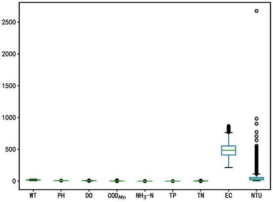
Figure 3.
Box diagram of the water quality data before outlier processing.
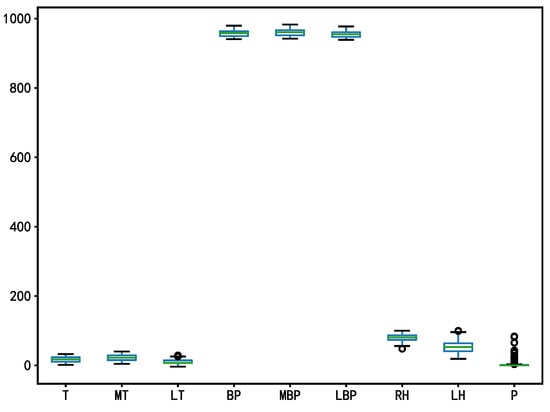
Figure 4.
Box diagram of the meteorological data before outlier processing.
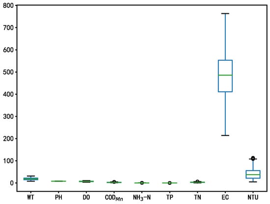
Figure 5.
Box diagram of the water quality data after outlier processing.
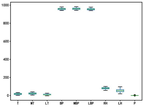
Figure 6.
Box diagram of the meteorological data after outlier processing.
3. Results and Discussion
3.1. Results Analysis of Variational Mode Decomposition
Water quality is affected by different factors. Water quality data is composed of the entangled data of different frequency bands. Different frequency bands have different characteristics. Variational mode decomposition can be used to separate the signals of different frequency bands from the original data in order to find the research laws better. Figure 7 is a comparison diagram of the original data and various signals, in which IMF1 is a low-frequency signal representing the long-term trend of the data, and IMF2-5 is a high-frequency signal representing the short-term mutation of the data. Figure 8 is the Fourier spectrum diagram after DO variational mode decomposition, which is the spectrum diagram of each signal obtained using Fourier transformation. Figure 8 shows that there is basically no frequency band entanglement among the signals after the decomposition of the DO water quality data, while the signals with the frequency band entanglement in the original data are effectively separated so as to be used for further research.
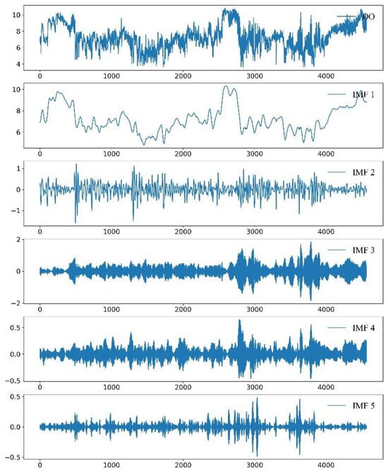
Figure 7.
Line diagram of the raw data and decomposed signal.
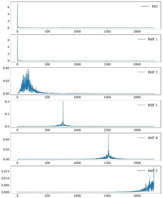
Figure 8.
Fourier spectrum diagram of the raw data and decomposed signal.
3.2. Correlation Analysis
The correlation between the variables was analyzed using the Pearson correlation analysis method. The correlation values between DO and the meteorological factors, pollution factors, and other variables in the original data and decomposed signals IMF1-IMF5 were obtained. The data list is shown in Table 4. Significance statistics were calculated automatically, and p-values were generated accordingly. The validity of the correlation coefficients was determined by checking whether the p-value was less than 0.05. All the correlation coefficients greater than 0.3 had p-values less than 0.05, which confirms the validity of the correlation analysis. The p-value of the statistical significance of the correlation coefficient is shown in Table 5.

Table 4.
The correlation values between DO and the variables in the raw data and decomposed signals IMF1-IMF5.

Table 5.
The p-values of statistical significance of the correlation coefficients.
It is generally believed that variables with an absolute value of correlation less than 0.3 are not correlated, 0.3–0.8 are relatively strongly correlated, and greater than 0.8 are very strongly correlated [33]. Based on the correlation analysis and VMD decomposition, the main factors influencing the long-term and short-term dissolved oxygen content could be determined.
The results show that the long-term trend characteristic of DO is influenced by the superposition of meteorological factors, hydrological factors, and water pollution factors, but it is not strongly correlated with any single factor. The absolute value of correlations between WT, T, TP, MT, MBP, BP, LBP, PH, CODMn, NH3-N, and DO are 0.3–0.8, which indicates that these factors have a relatively strong influence on the long-term characteristics of DO. Among them, the influence of temperature, phosphorus, and air pressure are relatively higher, while the pH value, CODMn, and nitrogen are relatively lower. The other factors except the above have weak correlations or no correlations on the long-term trend of DO, according to the results. The short-term mutation characteristics of DO are mainly affected by the water temperature, pH value, and eutrophication factors, such as NH3-N, TP, and TN in water bodies, which indicates that the short-term mutation characteristics of DO are mainly determined by the characteristics of the water body itself, and so the influence of the meteorological factors can basically be ignored.
3.3. Comparative Analysis of the Model Simulation Results before and after Decomposition
3.3.1. Model Simulation Results with the Original Data
Three models, the GRU, random forest, and XGBoost, were used to predict the DO content in the Chengdu area with the original data. The results are shown in Figure 9.


Figure 9.
Simulated results with the original data.
The average absolute error (MAE), root mean square error (RMSE), and symmetric mean absolute percentage error (SMAPE) were used to evaluate the variation degree and accuracy of the three models so as to judge the prediction effect of all three models. The RMSE, MAE, and SMAPE were calculated as shown in Table 6.

Table 6.
The RMSE, MAE, and SMAPE of the simulation with the original data.
As seen in the table, the RMSE value is greater than 0.905, the SMAPE value is less than 0.104, and the MAE value, 0.519–0.742, is moderate. The evaluation results show that, affected by the interference factors, the fitting degree of the three models to the original data is relatively low, and the simulation effect is not so good.
3.3.2. Model Simulation Results with the Decomposed Signals
The signals whose correlation with the predicted target DO was less than 0.3 were deleted first. Then, using the signal data obtained from the mode decomposition of the other variables, the DO was predicted using the GRU, random forest, and XGBoost techniques. The simulation results are shown in Figure 10. The RMSE, MAE, and SMAPE were calculated in the same way. Their results are shown in Table 7.

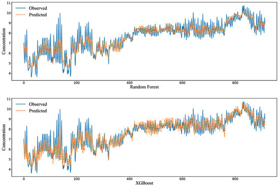
Figure 10.
Simulated results with the decomposed signals.

Table 7.
The RMSE, MAE, and SMAPE of the simulation with the decomposed signals.
Obviously, after eliminating the influence of the interference factors, the simulation results of the GRU, random forest, and XGBoost models significantly improved. The RSME value ranges from 0.482 to 0.511, the SMAPE value ranges from 0.052 to 0.059, and the MAE ranges from 0.364 to 0.435. All the values greatly improved compared with those before decomposition. The simulation results show that variational mode decomposition is very helpful to improve the simulation results. Additionally, the XGBoost and random forest models have a high simulation fitting degree and can be used to predict DO in the water environment of Chengdu.
3.4. Discussion
In this paper, a deep analysis of the original water quality data was conducted by combining variational mode decomposition with Fourier transformation. The analysis results indicate that the data consist of multiple modal signals at different frequencies, which may be related to various influencing factors on the water quality data, including the long-term trends caused by seasonal changes and short-term fluctuations due to occasional events. Based on this, an innovative water quality prediction framework for DO prediction was developed by combining VMD with machine learning and deep learning techniques. In this framework, the original data were initially decomposed into several intrinsic mode components, and these intrinsic mode components were filtered out subsequently by using a filter. Then, by combining intelligent models, the relationship between the intrinsic mode components and DO was explored to predict future changes. The prediction results of the GRU, random forest, and XGBoost models with and without the framework constructed in this paper were compared in order to verify the effectiveness of the framework. The prediction evaluation metrics were the RMSE, MAE, and SMAPE. The experimental results demonstrated that the prediction accuracy of the GRU deep learning model was improved by 27.56%, 16.4%, and 16.5% for the RMSE, MAE, and SMAPE, respectively. The improvement effect of the machine learning model was more obvious. The random forest was improved by 44.5%, 47.8%, and 46.8%, and XGBoost by 46.8%, 49.3%, and 48.4%. The obvious improvement of the machine learning model may be attributed to VMD separating the entangled modal signals from the original data, obtaining the modal components representing different frequency bands, preventing the essential change patterns of the data from being obscured by the entangled modes, using the filter to eliminate the noise unrelated to DO, and thereby enhancing the prediction accuracy. Through the constructed framework, the machine model can capture the inherent law of complex non-linear water quality sequence data more accurately, which causes the prediction accuracy of the machine model to exceed the deep learning model. This verifies the effectiveness of the framework. In addition, through the constructed framework, the inherent law of complex non-linear water quality sequence data can be more accurately captured using the machine learning model so that the prediction accuracy even exceeds the GRU deep learning model, which further verifies the effectiveness of the framework.
4. Conclusions
The correlation analysis between the influencing factors and DO in the water environment in the Chengdu area was carried out. It was concluded that the long-term trend characteristic of DO is influenced by the superposition of meteorological factors, hydrological factors, and water pollution factors. The air temperature, water temperature, phosphorus, air pressure, pH value, chemical oxygen demand, and nitrogen are relatively strongly correlated with the long-term trend characteristics of DO. Further, a signal decomposition analysis was carried out using the VMD method. It was concluded that only the water characteristics, such as the water temperature, pH value, and eutrophication gradients, have the greatest influence on the short-term mutation characteristics of DO. By combining frequency division with GRU, random forest, and XGBoost models, the DO content was predicted before and after variational mode decomposition. It was found that variational mode decomposition could effectively improve the simulation accuracy of the model.
DO is only one of the factors that can be used to measure environmental water quality. In future studies, we can try to further explore the actual impact of variational mode decomposition on the prediction models of various pollution factors that are not DO. We could attempt to develop a new water quality forecasting model system using variational mode decomposition combined with a water quality prediction model. The application scope of the new forecasting model system could also be extended from the Chengdu area to a larger regional scope.
Author Contributions
Methodology, K.C.; Investigation, M.L.; Data curation, D.W.; Writing—original draft, M.L.; Writing—review & editing, M.L. and R.X.; Supervision, R.X. All authors have read and agreed to the published version of the manuscript.
Funding
This research is supported by the National Natural Science Foundation (52050410328), the Guangxi Natural Science Foundation (2021GXNS FAA220056), and the National Natural Science Foundation (62266014).
Data Availability Statement
Data are contained within the article.
Acknowledgments
We are grateful to the Key Laboratory of Drinking Water Source Protection in the Chengdu Basin of the Sichuan Province, Chengdu University, for providing their support in conducting this research.
Conflicts of Interest
The authors declare no conflict of interest.
References
- Marc, W.B.; Theo, M.L.; Stephen, R.D.; Barry, C.M. Effects of aerobic and anaerobic conditions on P, N, Fe, Mn, and Hg accumulation in waters overlaying profundal sediments of an oligo-mesotrophic lake. Water Res. 2008, 42, 1953–1962. [Google Scholar]
- Wang, R.; Wang, T.; Qu, G.; Guo, X.; Jia, H.; Zhu, L. Insights into the underlying mechanisms for integrated inactivation of A. spiroides and depression of disinfection byproducts by plasma oxidation. Water Res. 2021, 196, 117027. [Google Scholar] [CrossRef]
- Han, J.; Cao, R.; Li, K.; Wang, S.; Ji, G.; Xu, H.; Wang, J.; Huang, T.; Wen, G. Change of algal organic matter under different dissolved oxygen and pressure conditions and its related disinfection by-products formation potential in metalimnetic oxygen minimum. Water Res. 2022, 226, 119216. [Google Scholar] [CrossRef]
- Shi, P.; Li, G.; Yuan, Y.; Huang, G.; Kuang, L. Prediction of dissolved oxygen content in aquaculture using Clustering based Soft plus Extreme Learning Machine. Comput. Electron. Agric. 2019, 157, 329–338. [Google Scholar] [CrossRef]
- Sun, L.; Wu, Y.; Li, D.; Wang, B.; Sun, X.; Luo, B. Prediction model for the number of crucian carp hypoxia based on the fusion of fish behavior and water environment factors. Comput. Electron. Agric. 2021, 189, 106386. [Google Scholar] [CrossRef]
- Yin, L.; Fu, L.; Wu, H.; Xia, Q.; Jiang, Y.; Tan, J.; Guo, Y. Modeling dissolved oxygen in a crab pond. Ecol. Model. 2021, 440, 109385. [Google Scholar] [CrossRef]
- Yan, X.; Han, H.; Li, X.; Wen, X.; Rong, X.; Xia, Y.; Yan, X. Dissolved organic carbon and dissolved oxygen determine the nitrogen removal rate constant in small water bodies of intensive agricultural region. Agric. Ecosyst. Environ. 2024, 361, 108822. [Google Scholar] [CrossRef]
- Ariely, C.; Ruben, C.; Sara, N.; Cristina, M.O.; Ricardo, J.N. Determination of dissolved oxygen in water by the Winkler method: Performance modelling and optimisation for environmental analysis. Microchem. J. 2021, 165, 106129. [Google Scholar]
- Sudipto, M.; Manojit, D.; Santanu, R.; Phani, B.G.; Madhumita, R.; Samit, R. Dynamic modelling of dissolved oxygen in the creeks of Sagar island, Hooghly–Matla estuarine system, West Bengal, India. Appl. Math. Model. 2012, 36, 5952–5963. [Google Scholar]
- Feng, M.L.; SUN, T.; Zhang, L.X.; Shen, X.M. Net Ecosystem Metabolism Simulation by Dynamic Dissolved Oxygen Model in Yellow River Estuary, China. Procedia Environ. Sci. 2012, 13, 807–817. [Google Scholar] [CrossRef][Green Version]
- Omnia, A.; Elena, M.; Mohie, O.; Reinhard, H. Numerical simulation of Dissolved Oxygen as a water quality indicator in artificial lagoons-Case study El Founa, Egypt. Reg. Stud. Mar. Sci. 2022, 56, 102697. [Google Scholar]
- Crossman, J.; Futter, M.N.; Elliott, J.A.; Whitehead, P.G.; Jin, L.; Dillon, P.J. Optimizing land management strategies for maximum improvements in lake dissolved oxygen concentrations. Sci. Total Environ. 2019, 652, 382–397. [Google Scholar] [CrossRef]
- Liu, Y.L. Simulation Study on Agricultural Non-Point Source Pollution in Xiaowei River Basin Based on SWAT Model. Master’s Thesis, Chang’an University, Xi’an, China, 2023; pp. 6–8. [Google Scholar]
- Mou, L.T.; Philio, W.G.; Yang, X.; James, H. A review of SWAT applications, performance and future needs for simulation of hydro-climatic extremes. Adv. Water Resour. 2020, 143, 103662. [Google Scholar]
- Xu, R.; Wu, W.; Cai, Y.; Wan, H.; Li, J.; Zhu, Q.; Shen, S. Feature Extraction and Prediction of Water Quality Based on Candlestick Theory and Deep Learning Methods. Water 2023, 15, 845. [Google Scholar] [CrossRef]
- Zhu, M.; Wang, J.; Yang, X.; Zhang, Y.; Zhang, L.; Ren, H.; Wu, B.; Ye, L. A review of the application of machine learning in water quality evaluation. Eco-Environ. Health 2022, 1, 107–116. [Google Scholar] [CrossRef]
- Singh, K.P.; Basant, A.; Malik, A.; Jain, G. Artificial neural network modeling of the river water quality—A case study. Ecol. Model. 2009, 220, 888–895. [Google Scholar] [CrossRef]
- Selim, A.; Shuvo, S.N.A.; Islam, M.M.; Moniruzzaman, M.; Shah, S.; Ohiduzzaman, M. Predictive models for dissolved oxygen in an urban lake by regression analysis and artificial neural network. Total Environ. Res. Themes 2023, 7, 100066. [Google Scholar] [CrossRef]
- Ahmed, A.A.M. Prediction of dissolved oxygen in Surma River by biochemical oxygen demand and chemical oxygen demand using the artificial neural networks (ANNs). J. King Saud Univ. Eng. Sci. 2017, 29, 151–158. [Google Scholar] [CrossRef]
- Bourel, M.; Segura, A.M.; Crisci, C.; Lopez, G.; Sampognaro, L.; Vidal, V.; Kruk, C.; Piccini, C.; Perera, G. Machine learning methods for imbalanced data set for prediction of faecal contamination in beach waters. Water Res. 2021, 202, 117450. [Google Scholar] [CrossRef]
- Heddam, S.; Kisi, O. concentration using least square support vector machine, multivariate adaptive regression splines and M5 model tree. J. Hydrol. 2018, 559, 499–509. [Google Scholar] [CrossRef]
- Nong, X.; Lai, C.; Chen, L.; Shao, D.; Zhang, C.; Liang, J. Prediction modelling framework comparative analysis of dissolved oxygen concentration variations using support vector regression coupled with multiple feature engineering and optimization methods: A case study in China. Ecol. Indic. 2023, 146, 109845. [Google Scholar] [CrossRef]
- Li, C.; Li, Z.; Wu, J.; Zhu, L.; Yue, J. A hybrid model for dissolved oxygen prediction in aquaculture based on multi-scale features. Inf. Process. Agric. 2018, 5, 11–20. [Google Scholar] [CrossRef]
- Chen, L.; Wu, T.; Wang, Z.; Lin, X.; Cai, Y. A novel hybrid BPNN model based on adaptive evolutionary Artificial Bee Colony Algorithm for water quality index prediction. Ecol. Indic. 2023, 146, 109882. [Google Scholar] [CrossRef]
- Lecun, Y.; Bengio, Y.; Hinton, G. Deep learning. Nature 2015, 521, 436–444. [Google Scholar] [CrossRef]
- Fang, Z.; Crimier, N.; Scanu, L.; Midelet, A.; Alyafi, A.; Delinchant, B. Multi-zone indoor temperature prediction with LSTM-based sequence to sequence model. Energy Build. 2021, 245, 111053. [Google Scholar] [CrossRef]
- Huan, J.; Li, H.; Li, M.; Chen, B. Prediction of dissolved oxygen in aquaculture based on gradient boosting decision tree and long short-term memory network: A study of Chang Zhou fishery demonstration base, China. Comput. Electron. Agric. 2020, 175, 105530. [Google Scholar] [CrossRef]
- Li, W.; Wu, H.; Zhu, N.; Jiang, Y.; Tan, J.; Guo, Y. Prediction of dissolved oxygen in a fishery pond based on gated recurrent unit (GRU). Inf. Process. Agric. 2021, 8, 185–193. [Google Scholar] [CrossRef]
- Chung, J.; Gulcehre, C.; Cho, K.H.; Bengio, Y. Empirical evaluation of gated recurrent neural networks on sequence modeling. arXiv 2014, arXiv:1412.3555. [Google Scholar]
- Fu, R.; Zhang, Z.; Li, L. Using LSTM and GRU neural network methods for traffic flow prediction. In Proceedings of the 31st Youth Academic Annual Conference of Chinese Association of Automation (YAC), Wuhan, China, 11–13 November 2016; IEEE: Piscataway, NJ, USA, 2016; pp. 324–328. [Google Scholar]
- Guo, J.; Dong, J.; Zhou, B.; Zhao, X.; Liu, S.; Han, Q.; Wu, H.; Xu, L.; Hassan, S.G. A hybrid model for the prediction of dissolved oxygen in seabass farming. Comput. Electron. Agric. 2022, 198, 106971. [Google Scholar] [CrossRef]
- Konstantin, D.; Dominique, Z. Variational Mode Decomposition. IEEE Trans. Signal Process. 2014, 62, 531–544. [Google Scholar]
- Jia, J. Statistics, 7th ed.; China Renmin University Press: Beijing, China, 2018. [Google Scholar]
Disclaimer/Publisher’s Note: The statements, opinions and data contained in all publications are solely those of the individual author(s) and contributor(s) and not of MDPI and/or the editor(s). MDPI and/or the editor(s) disclaim responsibility for any injury to people or property resulting from any ideas, methods, instructions or products referred to in the content. |
© 2024 by the authors. Licensee MDPI, Basel, Switzerland. This article is an open access article distributed under the terms and conditions of the Creative Commons Attribution (CC BY) license (https://creativecommons.org/licenses/by/4.0/).