Quantifying the Impacts of Dry–Wet Combination Events on Vegetation Vulnerability in the Loess Plateau under a Changing Environment

Abstract

Extreme drought and flood events, as well as their combined events, pose significant challenges to global sustainable socio-economic development and ecological health. However, the impact of dry–wet combination events (DWCEs) on vegetation vulnerability remains to be investigated. The Loess Plateau (LP) was selected as the study area to explore the response time of vegetation to precipitation index changes by optimal correlation coefficient; then, the impact of different DWCEs on vegetation vulnerability under moderate and severe scenarios was analyzed; finally, a vegetation loss probability model was constructed based on the copula function and Bayesian framework, to quantify the vegetation loss probability under DWCEs stress. The results indicate that: (1) normalized difference vegetation index (NDVI) shows an upward trend in spring, summer, and autumn, with the proportion of areas are 90.5%, 86.2%, and 95.4%, respectively, and show an insignificant trend in winter; (2) the response time of vegetation to precipitation index changes tends to be one or two seasons; (3) moderate scenarios have more influence than severe scenarios, dry-to-wet events (DWEs), wet-to-dry events (WDE) and continuous dry events (CDE) in spring-summer have a significant impact on summer vegetation of Ningxia and Shanxi, and WDE and CDE have a higher impact on autumn vegetation. (4) in terms of the probability of vegetation loss, DWE, and CDE cause higher losses to summer vegetation, while WDE and CDE cause higher losses to autumn vegetation. This study quantifies the impact of adjacent seasonal DWCE stress on future vegetation vulnerability.

1. Introduction

Droughts and floods, with their broad impact and frequent occurrence, post significant threats to the ecological environment, food security, economic development, and human health [1,2,3,4]. Under changing environments, drought and flood disasters with spatiotemporal correlation will occur continuously or interact with each other to develop into dry and wet combination events (DWCEs) [5,6], increasing the scope and intensity of the disaster and causing more serious losses to society.

The combination of dry and wet events includes a sudden transition from drought to flood and DWCEs [7]. The sudden transition from drought to flood refers to the phenomenon of rapid changes in drought and flood disasters in a very short period [8]. The DWCEs include dry-to-wet events (DWEs), wet-to-dry events (WDEs), continuous dry events (CDEs), and continuous wet events (CWEs) [9]. Compared to sudden changes in drought and flood events, DWCEs occur more frequently and lead to more substantial losses. For example, He et al. [10] found that about 5.9% and 7.6% of the world’s land experienced DWE in spring–summer and autumn–winter, respectively. The DWCEs widely occurred in countries such as Australia [11], the United Kingdom [12], Peru [13], China [14], and so on, causing serious impacts on the economy, environment, and food security. Taking China as a case example, the spring–summer drought that spanned from 2009 to 2010 in southwestern region led to economic losses exceeding CNY 19 billion. Similarly, the continuous drought that stretched across the winter, spring, and summer on the Loess Plateau (LP) from 1994 to 1995 inflicted economic damages amounting to CNY 6.675 billion [14]. Furthermore, the cumulative area impacted by the severe drought that persisted for six consecutive years in China, from 1978 to 1983, was 62 million hectares. More seriously, the frequency and intensity of seasonal CDE and CWE, as well as seasonal wet–dry alternation, will increase in the future [15,16,17]. Therefore, it is both necessary and urgent to investigate the potential impacts of DWCEs on various sectors, including ecology, economy, and society, within the context of a changing environment.

Previous studies have predominantly concentrated on examining the spatiotemporal distribution characteristics of combined dry and wet events [18,19,20,21,22,23]. However, few studies have focused on the impact of DWCE stress on vegetation vulnerability [24]. Given that vegetation coverage is influenced by climatic factors, including precipitation and temperature, it follows that both droughts and floods exert a notable effect on plant life [4,25,26]. Vegetation, as an important component of ecosystems, connects the cycles of carbon, water, and energy, determining the dynamic balance of global ecosystems [27]. However, different DWCEs have different effects on vegetation growth [28]. For instance, in the scenario of CDE, scarce water resources limit vegetation growth and even lead to vegetation apoptosis; but in the scenario of CWE, excessive water may cause vegetation stomata to be blocked, affecting the normal physiological functions of vegetation and leading to vegetation apoptosis. The rapid demise of vegetation can lead to a reduction in biomass, damage ecosystem diversity, trigger various secondary disasters, and threaten human survival and development. Therefore, it is of great significance to further evaluate vegetation vulnerability under DWCE stress.

Drought and floods are the two quintessential natural disasters in the LP. Despite its diverse array of vegetation types, the ecological environment here is exceedingly delicate, making it a key area for comprehensive soil and water conservation management in China [29,30,31]. Given the LP’s propensity for frequent droughts and floods, coupled with its fragile vegetation cover, it was selected as the study area. A considerable number of studies have explored the impact of drought and flood conditions on vegetation [26,32,33,34]. However, there is relatively little research on the impact of CDE and CWE on vegetation, while CDE and CWE may exacerbate the death of vegetation [35]. Therefore, to quantitatively evaluate the impact of DWCE stress on vegetation vulnerability in the LP, a model based on the copula function [36] and Bayesian conditional probability [37] was constructed to quantify the vegetation loss probability under all kinds of DWCE stress (DWE, WDE, CDE, and CWE). It is crucial for ensuring the sustainable management of water resources, providing strategic direction for agricultural practices, and formulating effective disaster mitigation tactics.

This study aims to evaluate the impact of DWCEs between adjacent seasons on vegetation vulnerability. Owning to factors such as climate type, land cover, agricultural production, and ecological environment, the LP is particularly sensitive to climate change and is one of the regions with the most concentrated contradictions in population, resources, and environment in China. Therefore, the specific objectives of this study are as follows: (1) evaluate the correlation between vegetation status and precipitation index, and determine the response time of vegetation to precipitation index changes; (2) identify sensitive areas of vegetation vulnerability response under DWCEs stress; (3) quantify the probability of vegetation loss under DWCEs stress based on the three-dimensional joint distribution model. This research framework is also applicable to other regions for evaluating vegetation loss probability and is beneficial for deepening the understanding of vegetation vulnerability under DWCE stress.

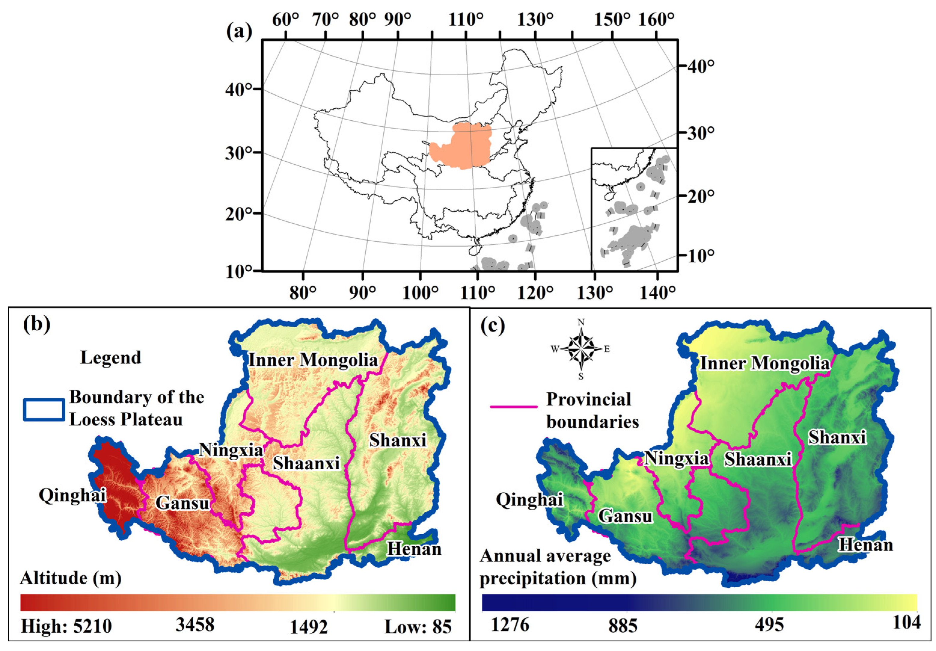
2. Study Area and Data

The LP is the second largest plateau in China, spanning from west to east across Qinghai, Gansu, Ningxia Hui Autonomous Region, Inner Mongolia Autonomous Region, Shaanxi, Shanxi, and Henan Province (Figure 1) [38]. The LP is characterized by a temperate continental monsoon climate, with an average annual precipitation of 466 mm that diminishes from the southeast to the northwest [39]. Specifically, the southern region receives 600–700 mm of rainfall, the central area receives 300–400 mm, and the northwest region receives only 100–200 mm. Seasonally, the LP is affected by the Western Pacific subtropical high and the Indian Ocean low during summer and autumn, leading to hot temperatures and frequent rainstorms. In contrast, during the winter and spring, it is affected by polar dry and cold air masses, resulting in cold, dry conditions often accompanied by windy and sandy weather. Therefore, the LP experiences its peak precipitation levels during summer, with a heightened frequency of rainstorms in July and August, and extended periods of rainfall in September, which can easily lead to flood disasters. Conversely, the winter and spring months are marked by minimal precipitation, which can readily result in drought conditions.

The terrain of the LP is higher in the northwest and lower in the southeast, with an average altitude of 1400 m. The vegetation coverage in the LP is influenced by factors such as latitude, water, altitude, and energy, and from southeast to northwest, it is sequentially divided into warm temperate sub-humid deciduous broad-leaved forest areas, warm temperate semi-arid grassland areas, and mid temperate arid and semi-desert areas. Among them, the deciduous broad-leaved forest belt is mainly agricultural and suitable for planting drought-resistant crops; The semi-desert region is a semi-pastoral and semi-agricultural region dominated by animal husbandry, and the planting industry relies on irrigation. In addition, the southern part of the LP is adjacent to deciduous broad-leaved forests and mixed evergreen broad-leaved forests, while the western part transitions to the vegetation belt of the Qinghai Tibet Plateau, where various types of mountain vegetation are developed.

The meteorological data came from the precipitation products of the Global Land Data Assimilation System (https://search.earthdata.nasa.gov/search?q=GLDAS/, (accessed on 1 December 2023)). The precipitation data spans from 1981 to 2015, with a monthly time scale and a spatial scale of 0.25° × 0.25°. Due to the selected GLDAS-V2.0 time being only up to 2014, the 2015 monthly precipitation data was supplemented with GLDAS-V2.1 precipitation data [40]. In terms of vegetation data, GIMMS NDVI 3g, SPOT NDVI, and MODIS NDVI are currently highly valued and widely used vegetation index datasets. Among them, the GIMMS NDVI 3g dataset is the world’s longest continuous NDVI dataset (https://climatedataguide.ucar.edu/climate-data/ndvi-normalized-difference-vegetation-index-3rd-generation-nasagfsc-gimms, (accessed on 10 December 2023)), with a period of 1982 to 2015, a spatial resolution of 1/12 degrees, and a temporal resolution of 15 days. GIMMS NDVI 3g dataset was selected to characterize the spatial characteristics, change status, and response of vegetation to dry and wet changes because it has superior quality after preprocessing and has been widely used in regional and global scale vegetation dynamic change research [41].

3. Methods

3.1. Mann–Kendall Trend Test

The Mann–Kendall test is a non-parametric test method recommended by the World Meteorological Organization, which has been widely used in hydro-meteorological series [42], such as precipitation, temperature, and pressure. Due to its strong applicability (without limiting sample distribution and being unaffected by a few outliers) and convenient calculation, the Mann–Kendall trend analysis method was adopted to analyze the trend of the normalized vegetation index (NDVI).

3.2. The Response Time of Vegetation on Dry and Wet Variation

The standardized precipitation index (SPI) is an indicator representing the probability of precipitation occurrence in a certain period, which was first proposed to assess climate and drought change [43]. It has the advantages of simple calculation, strong stability, and can eliminate the temporal and spatial difference of precipitation [44]. In addition, SPI is sensitive to changes in drought and is suitable for drought assessment above the monthly scale.

The Pearson correlation analysis is commonly used for quantifying the strength of the association between two variables [45]. In this study, the response time of vegetation to the change in SPI was estimated based on the Pearson correlation analysis. Among them, the larger the correlation coefficient, the more significant the impact of dry and wet changes on vegetation conditions, and the longer the lag time, indicating that vegetation can resist long-term drought. The range of values for the correlation coefficient is [−1, 1]. Therefore, the response time of vegetation to SPI changes is defined as the lag time (seasonal scale) between SPI and NDVI when the absolute value of the correlation coefficient is maximum.

3.3. Frequency Statistical Method for Vegetation Vulnerability

The classification criteria for the SPI index are shown in

Table 1. The standard for classifying wet–dry levels.

SPI Value	Dry–Wet Degree
SPI ≤ −2.0	Extreme drought
−2.0 < SPI ≤ −1.5	Severe drought
−1.5 < SPI ≤ −1.0	Moderate drought
−1.0 < SPI ≤ 1.0	Near normal
1.0 < SPI ≤ 1.5	Moderate moist
1.5 < SPI ≤ 2.0	Severe moist
SPI > 2.0	Extreme moist

, based on which the dry and wet levels at the seasonal scale are divided. In this paper, a seasonal scale SPI (three months of cumulative precipitation) is calculated to characterize the degree of dryness and wetness of seasons.

To evaluate the impact of different DWCEs in adjacent seasons on vegetation vulnerability, dry and wet events in moderate and severe scenarios were extracted grid by grid, and corresponding grid proportions were counted.

$${\mathrm{P}}_{\mathrm{i}}=\frac{\mathrm{n}}{\mathrm{N}}$$

(1)

Among them, ${\mathrm{P}}_{\mathrm{i}}$ represents the impact of DWCEs on vegetation vulnerability; N is the number of grids in which moderate and severe combined dry and wet events occur; n is the number of NDVI < NDVI^40th when DWCEs occur. In addition, ${\mathrm{P}}_{\mathrm{i}}=0$ represents there is no DWCE; the larger the value of ${\mathrm{P}}_{\mathrm{i}}$, the greater the impact of DWCEs on vegetation vulnerability. NDVI^40th usually refers to the 40th percentile value of the NDVI. The 40th percentile of NDVI means that in a set of NDVI data, 40% of the data points have NDVI values below this 40th percentile value, while 60% of the data points have NDVI values above it.

3.4. Probability Assessment Model for Vegetation Loss

The copula function can describe the dependency relationship between variables and construct flexible multivariate joint distribution, which has been widely used in research on droughts, floods, rainstorms, etc. [46,47,48,49,50]. Meanwhile, Bayesian models are suitable for analyzing and expressing uncertain things, providing a solution for joint data analysis, and are widely used in hydrological and meteorological research [51,52,53]. Therefore, we combine the copula function with the Bayesian framework to construct a probability assessment model for vegetation loss, and the corresponding flowchart is shown in Figure 2.

• Univariate marginal distribution

The fitting and optimization of the marginal distribution is the first step in constructing the copula joint distribution function. Gamma, Normal, generalized Pareto, Weibull, and Gumbel distribution functions were widely used, which were selected in this study to fit the marginal distribution function of the NDVI series. Then, the Kolmogorov–Smirnov (K-S) test [54] and root mean square error (RMSE) minimum criterion were adopted to determine the optimal marginal distribution of NDVI. In terms of the SPI series, it was fitting by normal distribution because SPI is a standardized index.

2.

Binary copula joint distribution function

Assuming that the optimal marginal distribution functions of SPI and NDVI sequences are $\mathrm{u}={\mathrm{F}}_{\mathrm{S}\mathrm{P}\mathrm{I}}(\mathrm{s}\mathrm{p}\mathrm{i})$ and $\mathrm{v}={\mathrm{F}}_{\mathrm{N}\mathrm{D}\mathrm{V}\mathrm{I}}(\mathrm{n}\mathrm{d}\mathrm{v}\mathrm{i})$, their joint distribution is as follows [55]:

$${\mathrm{F}}_{\mathrm{S}\mathrm{P}\mathrm{I},\mathrm{N}\mathrm{D}\mathrm{V}\mathrm{I}}(\mathrm{s}\mathrm{p}\mathrm{i},\mathrm{n}\mathrm{d}\mathrm{v}\mathrm{i})=\mathrm{C}({\mathrm{F}}_{\mathrm{S}\mathrm{P}\mathrm{I}}(\mathrm{s}\mathrm{p}\mathrm{i}),{\mathrm{F}}_{\mathrm{N}\mathrm{D}\mathrm{V}\mathrm{I}}(\mathrm{n}\mathrm{d}\mathrm{v}\mathrm{i}))=\mathrm{C}(\mathrm{u},\mathrm{v})$$

(2)

Clayton–copula, Frank–copula, Gumbel–copula, Gaussian–copula, and t-copula were selected to construct joint distribution models, and their expressions are shown in

Table 2. Expressions of bivariate copula joint distribution function.

Copulas	$\mathbf{C}(\mathbf{u},\mathbf{v})$	Parameter Range
Clayton-Copula	${\max \left(\right[\mathrm{u}}^{-\mathsf{\theta }}{+\mathrm{v}}^{-\mathsf{\theta }}{-1]}^{-1/\mathsf{\theta }},0)$	$(-1,\infty )\backslash \left\{0\right\}$
Frank-Copula	$-\frac{1}{\mathsf{\theta }}\mathrm{l}\mathrm{n}(1+\frac{({\mathrm{e}}^{-\mathsf{\theta }\mathrm{u}}-1)({\mathrm{e}}^{-\mathsf{\theta }\mathrm{v}}-1)}{{\mathrm{e}}^{-\mathsf{\theta }}-1})$	$(-\infty ,\infty )\backslash \left\{0\right\}$
Gumbel-Copula	${\exp (-[(-\mathrm{lnu})}^{\mathsf{\theta }}{+(-\mathrm{lnv})}^{\mathsf{\theta }}{]}^{1/\mathsf{\theta }})$	$[1,\infty )$
Gaussian-Copula	${\displaystyle {\int }_{-\infty }^{{\mathrm{f}}^{-1}\left(\mathrm{u}\right)}{\displaystyle {\int }_{-\infty }^{{\mathrm{f}}^{-1}\left(\mathrm{v}\right)}\frac{1}{2\mathsf{\pi }\sqrt{{1-\mathsf{\theta }}^2}}}}\exp [-\frac{{\mathrm{s}}^2{-2\mathsf{\theta }\mathrm{st}+\mathrm{t}}^2}{{2(1-\mathsf{\theta }}^2)}]\mathrm{dsdt}$	$(-1,1)$
t-Copula	${\displaystyle {\int }_{-\infty }^{{\mathrm{t}}_{\mathrm{k}}^{-1}(\mathrm{u})}{\displaystyle {\int }_{-\infty }^{{\mathrm{t}}_{\mathrm{k}}^{-1}(\mathrm{v})}\frac{1}{2\mathsf{\pi }\sqrt{1-{\mathsf{\theta }}^2}}\mathrm{e}\mathrm{x}\mathrm{p}{[1+\frac{{\mathrm{s}}^2-2\mathsf{\theta }\mathrm{s}\mathrm{t}+{\mathrm{t}}^2}{\mathrm{k}(1-{\mathsf{\theta }}^2)}]}^{-(\mathrm{k}+2)/2}\mathrm{d}\mathrm{s}\mathrm{d}\mathrm{t}}}$	$(-1,1)$

. The parameters of the copula function are estimated based on the maximum likelihood method [56]. Further, RMSE and Akaike information criterion (AIC) are adopted to optimize the copula function [57], and the corresponding formulas are as follows:

$$\mathrm{R}\mathrm{M}\mathrm{S}\mathrm{E}=\sqrt{\frac{1}{\mathrm{n}}{\displaystyle {\sum }_{\mathrm{i}=1}^{\mathrm{n}}{\left[\mathrm{P}\mathrm{c}(\mathrm{i})-\mathrm{P}\mathrm{o}(\mathrm{i})\right]}^2}}$$

(3)

$$\mathrm{A}\mathrm{I}\mathrm{C}=\mathrm{n}\mathrm{l}\mathrm{n}(\mathrm{M}\mathrm{S}\mathrm{E})+2\mathrm{m}$$

(4)

$${\mathrm{MSE}=\mathrm{E}(\mathrm{Pc}-\mathrm{Po})}^2=\frac{1}{\mathrm{n}-\mathrm{m}}{\displaystyle {\sum }_{\mathrm{i}=1}^{\mathrm{n}}{\left[\mathrm{Pc}\left(\mathrm{i}\right)-\mathrm{Po}\left(\mathrm{i}\right)\right]}^2}$$

(5)

among them, $\mathrm{P}\mathrm{c}$ is the value of copula; $\mathrm{Po}$ is the experience value; $\mathrm{n}$ is the sample size; $\mathrm{m}$ is the parameter estimation of copula function.

3

Three-dimensional copula joint distribution function

The expression for the ternary Gaussian–copula function is as follows:

$${\mathrm{C}(\mathrm{u}}_1{,\mathrm{u}}_2{,\mathrm{u}}_3;\rho {)=\mathsf{\Phi }}_{\rho }{(\mathsf{\Phi }}^{-1}{(\mathrm{u}}_1{),\mathsf{\Phi }}^{-1}{(\mathrm{u}}_2{),\mathsf{\Phi }}^{-1}{(\mathrm{u}}_3\left)\right)$$

(6)

The expression of the ternary t-copula function is as follows:

$${\mathrm{C}(\mathrm{u}}_1{,\mathrm{u}}_2{,\mathrm{u}}_3;\rho {,\mathrm{k})=\mathrm{t}}_{\rho ,\mathrm{k}}{(\mathrm{t}}_{\mathrm{k}}^{-1}{(\mathrm{u}}_1{),\mathrm{t}}_{\mathrm{k}}^{-1}{(\mathrm{u}}_2{),\mathrm{t}}_{\mathrm{k}}^{-1}{(\mathrm{u}}_3\left)\right)$$

(7)

among them, $\rho$ is a third-order symmetric positive definite matrix with all elements on the diagonal being 1; ${\mathsf{\Phi }}_{\rho }$ is the distribution function of the ternary standard normal distribution with a correlation coefficient matrix of $\rho$, whose marginal distributions are all standard normal distributions; ${\mathsf{\Phi }}^{-1}$ is the inverse function of the standard normal distribution function; ${\mathrm{t}}_{\rho ,\mathrm{k}}$ is the distribution function of the standard ternary t-distribution with a correlation coefficient matrix of $\rho$ and degrees of freedom of $\mathrm{k}$; ${\mathrm{t}}_{\mathrm{k}}^{-1}$ is the inverse function of a univariate t-distribution function with a degree of freedom of $\mathrm{k}$.

Therefore, assuming the marginal distribution functions of spring SPI, summer SPI, and NDVI are ${\mathrm{u}}_1{=\mathrm{F}}_{{\mathrm{SPI}}_1}{(\mathrm{spi}}_1)$, ${\mathrm{u}}_2{=\mathrm{F}}_{{\mathrm{SPI}}_2}{(\mathrm{spi}}_2)$, and ${\mathrm{u}}_3={\mathrm{F}}_{\mathrm{N}\mathrm{D}\mathrm{V}\mathrm{I}}(\mathrm{n}\mathrm{d}\mathrm{v}\mathrm{i})$, respectively. The joint distribution between spring SPI and summer SPI series is ${\mathrm{F}}_{{\mathrm{SPI}}_1{,\mathrm{SPI}}_2}{(\mathrm{spi}}_1{,\mathrm{spi}}_2)$; the joint distribution between spring SPI and NDVI series is ${\mathrm{F}}_{{\mathrm{SPI}}_1,\mathrm{NDVI}}{(\mathrm{spi}}_1,\mathrm{ndvi})$; the joint distribution between summer SPI and NDVI is ${\mathrm{F}}_{{\mathrm{SPI}}_2,\mathrm{NDVI}}{(\mathrm{spi}}_2,\mathrm{ndvi})$; the three-dimensional joint distribution of spring SPI, summer SPI, and NDVI is ${\mathrm{F}}_{{\mathrm{SPI}}_1{,\mathrm{SPI}}_2,\mathrm{NDVI}}{(\mathrm{spi}}_1{,\mathrm{spi}}_2,\mathrm{ndvi})$. According to the Sklar theorem, there exists a unique copula function:

$${\mathrm{F}}_{{\mathrm{SPI}}_1{,\mathrm{SPI}}_2,\mathrm{NDVI}}{(\mathrm{spi}}_1{,\mathrm{spi}}_2{,\mathrm{ndvi})=\mathrm{C}(\mathrm{F}}_{{\mathrm{SPI}}_1}{(\mathrm{spi}}_1{),\mathrm{F}}_{{\mathrm{SPI}}_2}{(\mathrm{spi}}_2{)\mathrm{F}}_{\mathrm{NDVI}}{\left(\mathrm{ndvi}\right))=\mathrm{C}(\mathrm{u}}_1{,\mathrm{u}}_2{,\mathrm{u}}_3)$$

(8)

Similarly, the parameters of ${\mathrm{F}}_{{\mathrm{SPI}}_1{,\mathrm{SPI}}_2,\mathrm{NDVI}}{(\mathrm{spi}}_1{,\mathrm{spi}}_2,\mathrm{ndvi})$ were estimated by the maximum likelihood method, and RMSE and AIC were applied to optimize the three-dimensional copula function.

4

Probability of vegetation loss under DWCE stress

To evaluate the impact of DWCEs on vegetation vulnerability, the following moderate and severe scenarios are defined based on the dry and wet level classification of the SPI index (

Table 3. Probabilities of combined dry and wet events under different scenarios.

Combinations	Moderate Scenario	Severe Scenario
From dry to wet	P (–1.5 < X ≤ –1, 1 < Y ≤ 1.5)	P (–2 < X ≤ –1.5, 1.5 < Y ≤ 2)
From wet to dry	P (1 < X ≤ 1.5, –1.5 < Y ≤ –1)	P (1.5 < X ≤ 2, –2 < Y ≤ –1.5)
Continuous dry	P (–1.5 < X ≤ –1, –1.5 < Y ≤ –1)	P (–2 < X ≤ –1.5, –2 < Y ≤ –1.5)
Continuous wet	P (1 < X ≤ 1.5, 1 < Y ≤ 1.5)	P (1.5 < X ≤ 2, 1.5 < Y ≤ 2)

).

When DWCEs occur in spring and summer, the probability expression for certain vegetation loss also occurs as follows:

$$\mathrm{P}(\mathrm{X}\le \mathrm{x}|\mathrm{Y}\le \mathrm{y},\mathrm{Z}\le \mathrm{z})=\frac{{\mathrm{C}(\mathrm{F}}_{\mathrm{X}}{\left(\mathrm{x}\right),\mathrm{F}}_{\mathrm{Y}}{\left(\mathrm{y}\right),\mathrm{F}}_{\mathrm{Z}}\left(\mathrm{z}\right))}{{\mathrm{C}(\mathrm{F}}_{\mathrm{Y}}{\left(\mathrm{y}\right),\mathrm{F}}_{\mathrm{Z}}\left(\mathrm{z}\right))}=\frac{{\mathrm{C}(\mathrm{u}}_1{,\mathrm{u}}_2{,\mathrm{u}}_3)}{{\mathrm{C}(\mathrm{u}}_2{,\mathrm{u}}_3)}$$

(9)

among them, X, Y, and Z are NDVI, spring SPI, and summer SPI time series, respectively; ${\mathrm{u}}_1{=\mathrm{F}}_{\mathrm{X}}\left(\mathrm{x}\right)$, ${\mathrm{u}}_2{=\mathrm{F}}_{\mathrm{Y}}\left(\mathrm{y}\right)$, and ${\mathrm{u}}_3{=\mathrm{F}}_{\mathrm{Z}}\left(\mathrm{z}\right)$ are optimal marginal distribution function of NDVI, spring SPI, and summer SPI, respectively; ${\mathrm{C}(\mathrm{F}}_{\mathrm{Y}}{\left(\mathrm{y}\right),\mathrm{F}}_{\mathrm{Z}}\left(\mathrm{z}\right))$ is the copula joint distribution of spring SPI and summer SPI sequences; ${\mathrm{C}(\mathrm{F}}_{\mathrm{X}}{\left(\mathrm{x}\right),\mathrm{F}}_{\mathrm{Y}}{\left(\mathrm{y}\right),\mathrm{F}}_{\mathrm{Z}}\left(\mathrm{z}\right))$ is the three-dimensional copula joint distribution function of spring SPI, summer SPI, and NDVI series.

In this study, the vegetation loss scenario is set as NDVI < NDVI^40th. The calculation formula for the vegetation loss probability under the DWE stress in a moderate scenario is presented as follows:

$$\mathrm{P}(\mathrm{X}\le \mathrm{x}|-1.5<\mathrm{Y}\le -1,1<\mathrm{Z}\le 1.5)=\mathrm{A}/\mathrm{B}$$

(10)

$$\begin{array}{c}{\mathrm{A}=\mathrm{C}(\mathrm{F}}_{\mathrm{X}}{\left(\mathrm{x}\right),\mathrm{F}}_{\mathrm{Y}}(-{1),\mathrm{F}}_{\mathrm{Z}}(1.5\left)\right)-{\mathrm{C}(\mathrm{F}}_{\mathrm{X}}{\left(\mathrm{x}\right),\mathrm{F}}_{\mathrm{Y}}(-{1),\mathrm{F}}_{\mathrm{Z}}\left(1\right))\\ \hspace{1em}\hspace{1em}\hspace{1em}-{\mathrm{C}(\mathrm{F}}_{\mathrm{X}}{\left(\mathrm{x}\right),\mathrm{F}}_{\mathrm{Y}}(-1{.5),\mathrm{F}}_{\mathrm{Z}}(1.5\left)\right)+{\mathrm{C}(\mathrm{F}}_{\mathrm{X}}{\left(\mathrm{x}\right),\mathrm{F}}_{\mathrm{Y}}(-1{.5),\mathrm{F}}_{\mathrm{Z}}\left(1\right))\end{array}$$

(11)

$${\mathrm{B}=\mathrm{C}(\mathrm{F}}_{\mathrm{Y}}(-{1),\mathrm{F}}_{\mathrm{Z}}(1.5\left)\right)-{\mathrm{C}(\mathrm{F}}_{\mathrm{Y}}(-{1),\mathrm{F}}_{\mathrm{Z}}\left(1\right))-{\mathrm{C}(\mathrm{F}}_{\mathrm{Y}}(-1{.5),\mathrm{F}}_{\mathrm{Z}}(1.5\left)\right)+{\mathrm{C}(\mathrm{F}}_{\mathrm{Y}}(-1{.5),\mathrm{F}}_{\mathrm{Z}}\left(1\right))$$

(12)

4. Results

4.1. The Spatial Distribution Characteristics of NDVI

The spatiotemporal distribution of seasonal NDVI on the LP is shown in Figure 3. Overall, NDVI shows significant spatial differences in spring, summer, and autumn, while NDVI is weaker in winter. There is a trend of increasing vegetation coverage from northwest to southeast, indicating that the vegetation coverage in the southeast is better than that in the northwest. Possible reasons are as follows: the precipitation in the LP gradually increases from northwest to southeast, while the annual evaporation decreases from northwest to southeast, resulting in a higher vegetation coverage in the southeast compared to the northwest. In addition, the vegetation types in the northwest are mainly farmland and grassland, with relatively sparse vegetation. However, limited water resources further limit the growth of vegetation, resulting in lower vegetation coverage in the northwest region of the LP.

The seasonal NDVI variation trend of the LP from 1982 to 2015 was analyzed using the Mann–Kendall trend analysis (Figure 4). In most areas, NDVI shows an upward trend in spring, summer, and autumn, with the proportion of areas 90.5%, 86.2%, and 95.4%, respectively, indicating that vegetation coverage in most areas has improved in spring, summer, and autumn. Furthermore, although 60% of the vegetation on the LP shows an upward trend in winter, it is not significant. This is because the coverage of winter vegetation also slowly increases with the increase in temperature. However, the impact of the Mongolian high-pressure system has led to a sharp drop in winter temperatures, reducing physiological processes such as the photosynthesis, respiration, and transpiration of vegetation.

4.2. Response Time of NDVI to SPI

The spatial distribution map of correlation coefficients between spring SPI and NDVI is shown in Figure 5. The area with a positive correlation (negative correlation) between spring SPI and spring NDVI (Lag-0) accounts for 72.9% (27.1%) of the total area, and the areas with a positive correlation are mainly concentrated in the western and northern regions; the area of positive correlation between spring SPI and summer NDVI (Lag-1) is 92.4%, which is significantly correlated in Ningxia and Inner Mongolia regions; the regions with a positive correlation (56.4%) between spring SPI and autumn NDVI (Lag-2) are concentrated in the northwest. The results above indicate that the more precipitation in spring, the more beneficial it is to vegetation growth in spring, summer, and autumn. The relationship between spring SPI and winter NDVI (Lag-3) shows a negative correlation in most areas (64.4%), indicating that a humid spring may correspond to poorer vegetation conditions in winter.

The correlation coefficient distribution between summer SPI and NDVI with different lag times is shown in Figure 6. The proportion of regions where NDVI in summer, autumn, and winter is positively correlated with summer SPI is 81.9%, 88.4%, and 91.9%, respectively. This indicates that precipitation has a promoting effect on vegetation cover in most areas of the LP. It is noted that the area where spring NDVI (Lag-3) is positively correlated (negatively correlated) with summer SPI is 51.5% (48.5%), indicating that summer precipitation changes have a positive effect (inhibitory effect) on spring vegetation cover in half of the LP. In terms of regional distribution, the regions with a negative correlation between summer NDVI (Lag-0) and summer SPI are concentrated in Qinghai and Gansu provinces; the regions with a negative correlation between autumn NDVI (Lag-1) and summer SPI are distributed in Shaanxi.

In summary, the response time of vegetation on the LP to SPI changes is generally one season scale. In terms of spring SPI, the positive correlation response time is on a seasonal scale, manifested in most areas of the western LP, while the negative correlation response time is on two seasonal scales, reflecting the southern part of the LP. In terms of summer SPI, the response time is on a seasonal scale, and except for the negative correlation in the central and southern parts of Shaanxi, most other regions are positively correlated. Therefore, precipitation changes in spring and summer have a significant impact on the vegetation vitality in summer and autumn.

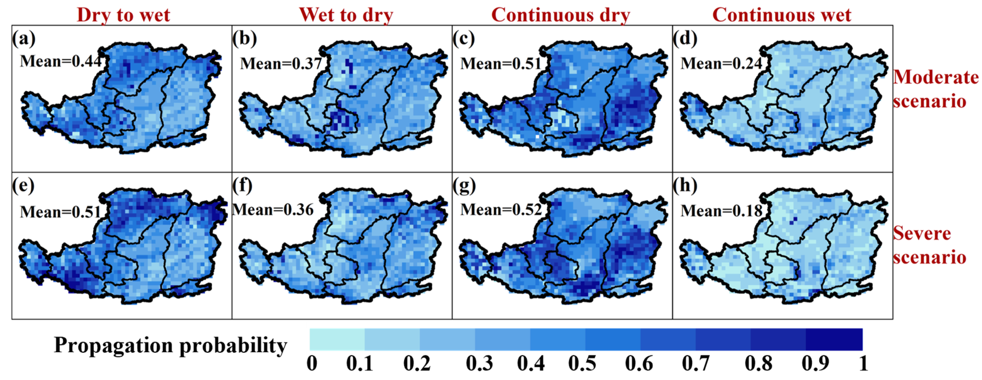
4.3. The Impact of DWCEs on Vegetation Vulnerability

4.3.1. The Impact on Summer Vegetation Vulnerability

Figure 7 shows the spatial distribution of the impact of spring–summer DWCEs on summer vegetation vulnerability. Results show that under moderate scenarios, the impacts of DWEs, WDEs, CDEs, and CWEs on summer vegetation vulnerability are 0.16, 0.14, 0.21, and 0.04, respectively. Under severe scenarios, the impacts of DWEs, WDEs, CDEs, and CWEs on summer vegetation vulnerability are 0.02, 0.05, 0.09, and 0.01, respectively. Results above indicate that CDEs have a greater impact on summer vegetation vulnerability and CWEs have a smaller impact on summer vegetation vulnerability under two kinds of scenarios. Overall, in terms of the influencing area, DWEs, WDEs, and CDEs under moderate scenarios and CDEs under severe scenarios are more severe than others.

The vulnerability of summer vegetation to spring–summer DWCEs under moderate and severe scenarios at the regional scale is listed in

Table 4. Effects of dry–wet combination events on summer vegetation vulnerability at the regional scale.

Combinations	Scenario	Gansu	Henan	Inner Mongolia	Ningxia	Qinghai	Shanxi	Shaanxi
Dry to wet	Moderate	0.11	0.52	0.09	0.55	0.09	0.16	0.08
	Severe	0.00	0.00	0.00	0.10	0.00	0.03	0.02
Wet to dry	Moderate	0.02	0.39	0.13	0.04	0.13	0.22	0.14
	Severe	0.08	0.06	0.01	0.00	0.00	0.05	0.09
Continuous dry	Moderate	0.15	0.23	0.23	0.63	0.00	0.27	0.07
	Severe	0.11	0.06	0.07	0.22	0.02	0.16	0.00
Continuous wet	Moderate	0.07	0.00	0.07	0.08	0.04	0.01	0.03
	Severe	0.00	0.00	0.02	0.00	0.00	0.00	0.01

Note: probability values greater than 0.5 are bolded.

. In terms of each region, under a moderate scenario, DWEs have a significant impact on the summer vegetation vulnerability in Henan (0.52) and Ningxia (0.55) and CDEs have a significant impact on the summer vegetation vulnerability in Ningxia (0.63). In addition, the impact of moderate WDEs, moderate CWEs, and severe DWCEs scenarios on summer vegetation vulnerability is relatively small (less than 0.5) in all provinces. In conclusion, the summer vegetation vitality in the Henan region is easily affected by moderate DWEs, while the summer vegetation vitality in the Ningxia region is easily affected by moderate DWEs and moderate CWEs.

4.3.2. The Impact on Autumn Vegetation Vulnerability

The impact of spring–summer DWCEs on autumn vegetation vulnerability can be seen in Figure 8. Under moderate scenarios, the impact of WDEs and CDEs on autumn vegetation vulnerability is greater, while the impact of moderate DWEs on autumn vegetation vulnerability is smaller. Under severe scenarios, the impact of WDEs and CDEs on autumn vegetation vulnerability is significant, while the impact of DWEs and CWEs on autumn vegetation vulnerability is relatively small. Overall, the impact of WDEs and CDEs on autumn vegetation vulnerability is significant, while the impact of CWEs and DWEs on autumn vegetation vulnerability in the entire region is relatively small.

Table 5. Effects of wet and dry combination events on autumn vegetation.

Combinations	Scenario	Gansu	Henan	Inner Mongolia	Ningxia	Qinghai	Shanxi	Shaanxi
Dry to wet	Moderate	0.02	0.19	0.05	0.29	0.05	0.08	0.01
	Severe	0.00	0.06	0.00	0.00	0.00	0.01	0.01
Wet to dry	Moderate	0.04	0.34	0.21	0.05	0.15	0.25	0.20
	Severe	0.09	0.10	0.16	0.03	0.02	0.13	0.04
Continuous dry	Moderate	0.14	0.19	0.22	0.60	0.00	0.13	0.11
	Severe	0.11	0.06	0.08	0.24	0.01	0.06	0.00
Continuous wet	Moderate	0.11	0.00	0.16	0.24	0.00	0.02	0.10
	Severe	0.00	0.00	0.02	0.00	0.00	0.00	0.04

Note: probability values greater than 0.5 are bolded.

shows the impact of DWCEs on autumn vegetation vulnerability from a provincial perspective. Only moderate CDEs have a significant impact on autumn vegetation vulnerability in Ningxia, the frequency is 0.6. Overall, the impact of DWCEs on autumn vegetation vulnerability is relatively small on the LP.

4.4. Probability of Vegetation Loss under DWCEs Stress

According to Section 4.2, vegetation in summer and autumn responds well to the precipitation changes in spring and summer. Therefore, this section aims to quantify the probability of loss of vegetation vulnerability in summer and autumn under moderate and severe spring-summer DWCEs stress, and mainly considering vegetation status NDVI < NDVI^40th.

4.4.1. Probability of Vegetation Loss in Summer

Figure 9 shows the spatial distribution of the probability of summer vegetation loss when DWCE occurs in spring and summer. From the perspective of mean value, when a DWE occurs, the probability of summer vegetation loss in moderate and severe scenarios is 0.44 and 0.51, respectively; when a WDE occurs, the probability of summer vegetation loss in moderate and severe scenarios is 0.37, and 0.36, respectively; The probability of summer vegetation loss is relatively high in moderate (0.51) and severe (0.52) scenarios when CDEs occur, respectively, indicating that summer vegetation under CDE stress is prone to loss; the probability of summer vegetation loss under moderate and severe CWEs is 0.24 and 0.18, respectively, indicating that the vulnerability of summer vegetation under CWEs stress is relatively low.

Overall, the impact of DWEs and CDEs on the summer vegetation vulnerability of the LP is significant, while the impact of CWEs and WDEs on the summer vegetation vulnerability of the watershed is relatively small. In addition, from moderate to severe scenarios, the probability of summer vegetation loss under stress from DWEs and CDEs increases, while the probability of summer vegetation loss under stress from WDEs and CWEs decreases. Therefore, severe DWEs, severe CDEs, moderate WDEs, and moderate CWEs have a significant impact on the vulnerability of summer vegetation.

In terms of each partition (

Table 6. Probability of vegetation loss in different zones during summer under the stress of spring-summer dry and wet combination events.

Combinations	Scenario	Gansu	Henan	Inner Mongolia	Ningxia	Qinghai	Shanxi	Shaanxi
Dry to wet	Moderate	0.50	0.46	0.54	0.47	0.45	0.38	0.36
	Severe	0.61	0.59	0.61	0.52	0.58	0.45	0.38
Wet to dry	Moderate	0.42	0.35	0.38	0.28	0.35	0.35	0.36
	Severe	0.34	0.41	0.36	0.25	0.34	0.40	0.37
Continuous dry	Moderate	0.43	0.49	0.46	0.59	0.45	0.58	0.50
	Severe	0.53	0.40	0.44	0.63	0.47	0.55	0.53
Continuous wet	Moderate	0.24	0.21	0.19	0.16	0.37	0.25	0.26
	Severe	0.14	0.13	0.18	0.11	0.27	0.18	0.22

Note: Probability values greater than 0.5 are bolded.

), taking the corresponding probability value of DWCEs greater than 0.5 as an example, partitions with a high probability of vegetation loss are as follows: Gansu and Inner Mongolia under a moderate DWE scenario; Gansu, Henan, Inner Mongolia, Ningxia, and Qinghai under a severe DWE scenario; Ningxia, Shanxi, and Shaanxi under a moderate CDE scenario; Gansu, Ningxia, Shanxi, and Shaanxi under a severe CDE scenario. It is worth noting that from moderate to severe scenarios, the probability of vegetation loss in DWEs is prone to increase, indicating that DWEs have an increased impact on the vulnerability of summer vegetation; The probability of vegetation loss for the other three combinations (WDEs, CEDs, and CWEs) shows a decreasing trend, indicating that the impact of these three types of DWCEs on the vulnerability of summer vegetation is weakened.

4.4.2. Probability of Vegetation Loss in Autumn

The impact of spring–summer DWCEs on autumn vegetation vulnerability is shown in Figure 10. Overall, WDEs and CDEs have a greater impact on autumn vegetation vulnerability, while CWEs and DWEs have a smaller impact on the overall autumn vegetation vulnerability. This conclusion is consistent with Section 4.3. This indicates that WDEs have a significant impact on the vitality of autumn vegetation. However, under the stress of CWEs, the fragility of autumn vegetation is relatively low. In addition, from moderate to severe scenarios, the probability of autumn vegetation loss under the stress of DWEs and WDEs increases, while the probability of autumn vegetation loss under the stress of CDEs and CWEs decreases. Therefore, it can be inferred that severe events such as DWEs, WDEs, moderate CDEs, and moderate CWEs have a significant impact on the vulnerability of autumn vegetation.

In terms of each partition (

Table 7. Probability of vegetation loss in different zones during autumn under the stress of spring-summer dry and wet combination events.

Combinations	Scenario	Gansu	Henan	Inner Mongolia	Ningxia	Qinghai	Shanxi	Shaanxi
Dry to wet	Moderate	0.28	0.30	0.36	0.33	0.32	0.28	0.30
	Severe	0.27	0.36	0.37	0.30	0.33	0.31	0.30
Wet to dry	Moderate	0.52	0.49	0.49	0.44	0.48	0.45	0.41
	Severe	0.64	0.65	0.56	0.47	0.57	0.56	0.46
Continuous dry	Moderate	0.44	0.39	0.42	0.54	0.52	0.55	0.38
	Severe	0.43	0.31	0.38	0.58	0.50	0.50	0.36
Continuous wet	Moderate	0.23	0.25	0.21	0.19	0.32	0.27	0.37
	Severe	0.17	0.16	0.21	0.14	0.25	0.22	0.36

Note: probability values greater than 0.5 are bolded.

), taking corresponding DWCEs with a probability value greater than 0.5 as an example, it is found that the probability of autumn vegetation loss in the following partitions is relatively high: Gansu under a moderate WDEs scenario; Gansu, Henan, Inner Mongolia, Qinghai, and Shanxi under severe WDEs scenario; Ningxia, Qinghai, and Shanxi under the background of moderate and severe CDEs. The above-mentioned DWCEs in these areas have a significant impact on autumn vegetation vulnerability.

5. Discussion

This study demonstrated a positive correlation between precipitation in spring and summer with subsequent vegetation growth, indicating that the growth status of vegetation in the LP is related to precipitation patterns. On a temporal scale, the response time is within 1–2 seasonal scales, which is consistent with the result of Li et al. [58]. The optimal response time to spring precipitation in the northwestern part of the LP is one season, while in the southern part, it is two seasons. This may be due to the fact that the northwestern part of the LP is drier than the southern part, with less local water storage and a more fragile ecological environment [59]. Therefore, in situations where vegetation is in a state of water scarcity and local water reserves are scarce, vegetation responds more quickly to changes in precipitation. In terms of summer precipitation, the response time of vegetation in most areas of the LP is one seasonal scale, which may be because of the rapid and lush growth of vegetation in summer, high water demand, and strong dependence of vegetation growth on precipitation. Meanwhile, due to high temperatures and increased evaporation, the vegetation has a greater demand for water. As a result, vegetation responding more sensitively and quickly to precipitation and quickly reflected through NDVI.

Under moderate scenarios, the results of the impact of spring–summer DWCEs on vegetation vulnerability indicate that the areas and average values of the impact of DWEs, WDEs, and CDEs on summer vegetation, as well as WDEs and CDEs on autumn vegetation, are relatively high. The affected areas are mainly distributed in Ningxia and Shanxi provinces, which confirms that different vegetation types on the LP [60] have differential responses to changes in precipitation. Wang et al. [60] found that farmlands have the weakest response to spring drought, which may be related to artificial irrigation and drought resistance, and moisture conservation activities, while grasslands and forests have the strongest response to spring drought. Combined with the results of this paper, it indicates that areas with strong human activities (such as the central and southern parts of the LP) are less susceptible to the impact of precipitation dynamics, and human activities to some extent mitigate the disturbance of moderate scenario precipitation on vegetation [61]. Under the DWEs, the frequency of vegetation vulnerability to precipitation in summer and autumn vegetation decreases, indicating that with the extension of lag time and the supply of water, the vegetation state improves; whereas under the WDEs and CDEs, the condition of vegetation does not improve with time lagging, which may be because, in the LP region of China, the soil moisture exhibits a pattern of “from dry to drier” [62], and only with precipitation to replenish can vegetation maintain normal growth. It is worth noting that the calculation results of the vegetation loss probability model constructed in this study also verify the above results.

6. Conclusions

LP is an important population and economic center in the northwest region of China, but with frequent natural disasters and a fragile and sensitive ecological environment. Therefore, analyzing the impact of DWCEs on vegetation vulnerability under changing environmental conditions is of guiding significance for promoting ecological protection and stable development of the LP. In this study, the optimal correlation coefficient was used to represent the response time of vegetation to SPI changes. The innovation of this study lies in the frequency statistical analysis of the impact of DWCE on vegetation vulnerability. Based on this, a vegetation loss probability evaluation model based on the copula function and Bayesian framework was constructed to quantitatively evaluate the probability of vegetation loss. The following conclusions were drawn:

• NDVI in spring, summer, and autumn showed a significant upward trend, with an area ratio of 90.5%, 86.2%, and 95.4%, respectively. However, the trend of NDVI changes in winter is not significant. The response time of vegetation changes to precipitation changes ranges from one to two seasons.
• The impact of DWCEs on vegetation vulnerability is greater in moderate scenarios than in severe scenarios. Specifically, DWEs, WDEs, and CDEs in spring–summer have a significant impact on the summer vegetation of Ningxia and Shanxi, and WDEs and CDEs have a higher impact on autumn vegetation.
• According to the mean value of the vegetation loss probability, the CDEs in the moderate scenario and DWEs and CDEs in the severe scenario cause significant losses to summer vegetation, with loss probabilities of 0.51, 0.51, and 0.52, respectively. WDEs and CDEs under moderate and severe scenarios have a significant impact on autumn vegetation loss, with a probability of loss ranging from 0.44 to 0.56. This study facilitates a better understanding of vegetation loss under DWCE stress. Furthermore, it provides a new framework for quantitatively assessing vegetation vulnerability, which is also applicable to other regions of the world.

References

1. Penning-Rowsell, E.C.; Yanyan, W.; Watkinson, A.R.; Jiang, J.; Thorne, C. Socioeconomic scenarios and flood damage assessment methodologies for the Taihu Basin, China. J. Flood Risk Manag. 2013, 6, 23–32. [Google Scholar] [CrossRef]
2. Elsey-Quirk, T.; Lynn, A.; Jacobs, M.D.; Diaz, R.; Cronin, J.T.; Wang, L.; Huang, H.; Justic, D. Vegetation dieback in the Mississippi River Delta triggered by acute drought and chronic relative sea-level rise. Nat. Commun. 2024, 15, 3518. [Google Scholar] [CrossRef] [PubMed]
3. Qiao, X.; Straight, B.; Ngo, D.; Hilton, C.E.; Owuor Olungah, C.; Naugle, A.; Lalancette, C.; Needham, B.L. Severe drought exposure in utero associates to children’s epigenetic age acceleration in a global climate change hot spot. Nat. Commun. 2024, 15, 4140. [Google Scholar] [CrossRef] [PubMed]
4. Dong, B.Q.; Qin, T.L.; Liu, S.S.; Liu, F.; Nie, H.J.; Wang, J.W.; Lv, Z.Y.; Shi, X.Q. Disentangling the Mutual Feedback Relationship between Extreme Drought and Flood Events and Ecological Succession of Vegetation. Pol. J. Environ. Stud. 2021, 30, 1003–1016. [Google Scholar] [CrossRef] [PubMed]
5. Meehl, G.A.; Tebaldi, C. More intense, more frequent, and longer lasting heat waves in the 21st century. Science 2004, 305, 994–997. [Google Scholar] [CrossRef] [PubMed]
6. Su, B.D.; Huang, J.L.; Fischer, T.; Wang, Y.J.; Kundzewicz, Z.W.; Zhai, J.Q.; Sun, H.M.; Wang, A.Q.; Zeng, X.F.; Wang, G.J.; et al. Drought losses in China might double between the 1.5 °C and 2.0 °C warming. Proc. Natl. Acad. Sci. USA 2018, 115, 10600–10605. [Google Scholar] [CrossRef] [PubMed]
7. Zhao, Y.; Weng, Z.H.; Chen, H.; Yang, J.W. Analysis of the Evolution of Drought, Flood, and Drought-Flood Abrupt Alternation Events under Climate Change Using the Daily SWAP Index. Water 2020, 12, 1969. [Google Scholar] [CrossRef]
8. Bi, W.X.; Li, M.; Weng, B.S.; Yan, D.H.; Dong, Z.Y.; Feng, J.M.; Wang, H. Drought-flood abrupt alteration events over China. Sci. Total Environ. 2023, 875, 162529. [Google Scholar] [CrossRef]
9. Hrdinka, T.; Novicky, O.; Hanslík, E.; Rieder, M. Possible impacts of floods and droughts on water quality. J. Hydro-Environ. Res. 2012, 6, 145–150. [Google Scholar] [CrossRef]
10. He, X.G.; Sheffield, J. Lagged Compound Occurrence of Droughts and Pluvials Globally Over the Past Seven Decades. Geophys. Res. Lett. 2020, 47, e2020GL087924. [Google Scholar] [CrossRef]
11. Verhoeven, E.; Wardle, G.M.; Roth, G.W.; Greenville, A.C. Characterising the spatiotemporal dynamics of drought and wet events in Australia. Sci. Total Environ. 2022, 846, 157480. [Google Scholar] [CrossRef] [PubMed]
12. Parry, S.; Marsh, T.; Kendon, M. 2012: From drought to floods in England and Wales. Weather 2013, 68, 268–274. [Google Scholar] [CrossRef]
13. Son, R.; Wang, S.Y.S.; Tseng, W.L.; Schuler, C.B.W.; Becker, E.; Yoon, J.H. Climate diagnostics of the extreme floods in Peru during early 2017. Clim. Dyn. 2020, 54, 935–945. [Google Scholar] [CrossRef]
14. Jin, G. Similarities and differences of hydrologic frequency distribution models and their parameter estimation problems. Adv. Water Sci. 2010, 21, 466–470. [Google Scholar]
15. Mu, W.B.; Yu, F.L.; Xie, Y.B.; Liu, J.; Li, C.Z.; Zhao, N.N. The Copula Function-Based Probability Characteristics Analysis on Seasonal Drought & Flood Combination Events on the North China Plain. Atmosphere 2014, 5, 847–869. [Google Scholar] [CrossRef]
16. Chen, J.; Dai, A.; Zhang, Y. Projected Changes in Daily Variability and Seasonal Cycle of Near-Surface Air Temperature over the Globe during the Twenty-First Century. J. Clim. 2019, 32, 8537–8561. [Google Scholar] [CrossRef]
17. Myoung, B.; Nielsen-Gammon, J.W. Sensitivity of monthly convective precipitation to environmental conditions. J. Clim. 2010, 23, 166–188. [Google Scholar] [CrossRef]
18. Shan, L.; Zhang, L.; Song, J.; Zhang, Y.; She, D.; Xia, J. Characteristics of dry-wet abrupt alternation events in the middle and lower reaches of the Yangtze River Basin and the relationship with ENSO. J. Geogr. Sci. 2018, 28, 1039–1058. [Google Scholar] [CrossRef]
19. Shi, X.; Guo, W.; Li, W.; Dai, S.; Lu, H. The sudden turn of drought and flood in spring in northern Qinghai Province, 2013: Characteristics and cause of formation. J. Glaciol. Geocryol. 2015, 37, 376–386. [Google Scholar]
20. Sun, C.; Yang, S. Persistent severe drought in southern China during winter–spring 2011: Large-scale circulation patterns and possible impacting factors. J. Geophys. Res. Atmos. 2012, 117, D10112. [Google Scholar] [CrossRef]
21. De Luca, P.; Messori, G.; Wilby, R.L.; Mazzoleni, M.; Di Baldassarre, G. Concurrent wet and dry hydrological extremes at the global scale. Earth Syst. Dyn. 2020, 11, 251–266. [Google Scholar] [CrossRef]
22. Zhang, X.; Alexander, L.; Hegerl, G.C.; Jones, P.; Tank, A.K.; Peterson, T.C.; Trewin, B.; Zwiers, F.W. Indices for monitoring changes in extremes based on daily temperature and precipitation data. WIREs Clim. Chang. 2011, 2, 851–870. [Google Scholar] [CrossRef]
23. Fang, W.; Huang, S.; Huang, G.; Huang, Q.; Wang, H.; Wang, L.; Zhang, Y.; Li, P.; Ma, L. Copulas-based risk analysis for inter-seasonal combinations of wet and dry conditions under a changing climate. Int. J. Climatol. 2019, 39, 2005–2021. [Google Scholar] [CrossRef]
24. Broich, M.; Tulbure, M.G.; Verbesselt, J.; Xin, Q.C.; Wearne, J. Quantifying Australia’s dryland vegetation response to flooding and drought at sub-continental scale. Remote Sens. Environ. 2018, 212, 60–78. [Google Scholar] [CrossRef]
25. Wang, Z.; Huang, Z.; Li, J.; Zhong, R.; Huang, W. Assessing impacts of meteorological drought on vegetation at catchment scale in China based on SPEI and NDVI. Trans. Chin. Soc. Agric. Eng. 2016, 32, 177–186. [Google Scholar]
26. Gao, Y.; Hu, T.; Yuan, H.; Yang, J. Analysis on yield reduced law of rice in Huaibei plain under drought-flood abrupt alternation. Trans. Chin. Soc. Agric. Eng. 2017, 33, 128–136. [Google Scholar]
27. Zhang, Q.; Han, L.Y.; Zeng, J.; Wang, X.; Lin, J.J. Climate factors during key periods affect the comprehensive crop losses due to drought in Southern China. Clim. Dyn. 2020, 55, 2313–2325. [Google Scholar] [CrossRef]
28. Chen, H.L.; Liang, Z.Y.; Liu, Y.; Jiang, Q.S.; Xie, S.G. Effects of drought and flood on crop production in China across 1949–2015: Spatial heterogeneity analysis with Bayesian hierarchical modeling. Nat. Hazards 2018, 92, 525–541. [Google Scholar] [CrossRef]
29. Zhang, B.; He, C.; Burnham, M.; Zhang, L. Evaluating the coupling effects of climate aridity and vegetation restoration on soil erosion over the Loess Plateau in China. Sci. Total Environ. 2016, 539, 436–449. [Google Scholar] [CrossRef]
30. Deng, L.; Kim, D.-G.; Li, M.; Huang, C.; Liu, Q.; Cheng, M.; Shangguan, Z.; Peng, C. Land-use changes driven by ‘Grain for Green’ program reduced carbon loss induced by soil erosion on the Loess Plateau of China. Glob. Planet. Chang. 2019, 177, 101–115. [Google Scholar] [CrossRef]
31. Sun, W.; Shao, Q.; Liu, J.; Zhai, J. Assessing the effects of land use and topography on soil erosion on the Loess Plateau in China. Catena 2014, 121, 151–163. [Google Scholar] [CrossRef]
32. Ullah, R.; Khan, J.; Ullah, I.; Khan, F.; Lee, Y. Assessing Impacts of Flood and Drought over the Punjab Region of Pakistan Using Multi-Satellite Data Products. Remote Sens. 2023, 15, 1484. [Google Scholar] [CrossRef]
33. Elagib, N.A.; Al Zayed, I.S.; Khalifa, M.; Rahma, A.E.; Ali, M.M.A.; Schneider, K. Drought versus flood: What matters more to the performance of Sahel farming systems? Hydrol. Process. 2023, 37, e14978. [Google Scholar] [CrossRef]
34. Marumbwa, F.M.; Cho, M.A.; Chirwa, P.W. An assessment of remote sensing-based drought index over different land cover types in southern Africa. Int. J. Remote Sens. 2020, 41, 7368–7382. [Google Scholar] [CrossRef]
35. Shi, W.Z.; Huang, S.Z.; Zhang, K.; Liu, B.J.; Liu, D.F.; Huang, Q.; Fang, W.; Han, Z.M.; Chao, L.J. Quantifying the superimposed effects of drought-flood abrupt alternation stress on vegetation dynamics of the Wei River Basin in China. J. Hydrol. 2022, 612, 128105. [Google Scholar] [CrossRef]
36. Shiau, J.T. Fitting Drought Duration and Severity with Two-Dimensional Copulas. Water Resour. Manag. 2006, 20, 795–815. [Google Scholar] [CrossRef]
37. Yang, W.T.; Zhang, L.Y.; Gao, Y. Drought and flood risk assessment for rainfed agriculture based on Copula-Bayesian conditional probabilities. Ecol. Indic. 2023, 146, 109812. [Google Scholar] [CrossRef]
38. Nie, M.; Huang, S.; Duan, W.; Leng, G.; Bai, G.; Wang, Z.; Huang, Q.; Fang, W.; Peng, J. Meteorological drought migration characteristics based on an improved spatiotemporal structure approach in the Loess Plateau of China. Sci. Total Environ. 2024, 912, 168813. [Google Scholar] [CrossRef] [PubMed]
39. Shi, H.; Shao, M. Soil and water loss from the Loess Plateau in China. J. Arid Environ. 2000, 45, 9–20. [Google Scholar] [CrossRef]
40. Song, H.; Zhu, Z.; Li, Y. Validation of land data assimilation and reanalysis precipitation datasets over Inner Mongolia. Arid Zone Res. 2021, 38, 1624–1636. [Google Scholar]
41. Brehaut, L.; Danby, R.K. Inconsistent relationships between annual tree ring-widths and satellite- measured NDVI in a mountainous subarctic environment. Ecol. Indic. 2018, 91, 698–711. [Google Scholar] [CrossRef]
42. Yan, J.J.; Zhang, G.P.; Ling, H.B.; Han, F.F. Comparison of time-integrated NDVI and annual maximum NDVI for assessing grassland dynamics. Ecol. Indic. 2022, 136, 108611. [Google Scholar] [CrossRef]
43. Mckee, T.B.; Doesken, N.J.; Kleist, J.R. The Relationship of Drought Frequency and Duration to Time Scales. In Proceedings of the 8th Conference on Applied Climatology, Anaheim, CA, USA, 17–22 January 1993. [Google Scholar]
44. Adnan, S.; Ullah, K.; Shuanglin, L.; Gao, S.; Khan, A.H.; Mahmood, R. Comparison of various drought indices to monitor drought status in Pakistan. Clim. Dyn. 2018, 51, 1885–1899. [Google Scholar] [CrossRef]
45. Pearson, K. Mathematical contributions to the theory of evolution—On a form of spurious correlation which may arise when indices are used in the measurement of organs. Proc. R. Soc. Lond. 1897, 60, 489–498. [Google Scholar] [CrossRef]
46. Xiao, M.X.; Yu, Z.B.; Zhu, Y.L. Copula-based frequency analysis of drought with identified characteristics in space and time: A case study in Huai River basin, China. Theor. Appl. Climatol. 2019, 137, 2865–2875. [Google Scholar] [CrossRef]
47. Mortuza, M.R.; Moges, E.; Demissie, Y.; Li, H.Y. Historical and future drought in Bangladesh using copula-based bivariate regional frequency analysis. Theor. Appl. Climatol. 2019, 135, 855–871. [Google Scholar] [CrossRef]
48. De Michele, C.; Salvadori, G.; Passoni, G.; Vezzoli, R. A multivariate model of sea storms using copulas. Coast. Eng. 2007, 54, 734–751. [Google Scholar] [CrossRef]
49. Wang, Z.; Huang, S.; Mu, Z.; Leng, G.; Duan, W.; Ling, H.; Xu, J.; Zheng, X.; Li, P.; Li, Z.; et al. Relative humidity and solar radiation exacerbate snow drought risk in the headstreams of the Tarim River. Atmos. Res. 2024, 297, 107091. [Google Scholar] [CrossRef]
50. Wei, X.; Huang, S.; Li, J.; Huang, Q.; Leng, G.; Liu, D.; Guo, W.; Zheng, X.; Bai, Q. The negative-positive feedback transition thresholds of meteorological drought in response to agricultural drought and their dynamics. Sci. Total Environ. 2024, 906, 167817. [Google Scholar] [CrossRef]
51. Zhang, Y.; Xiang, L.; Sun, Q.; Chen, Q. Bayesian Probabilistic Forecasting of Seasonal Hydrological Drought Based on Copula Function. Sci. Geogr. Sin. 2016, 36, 1437–1444. [Google Scholar]
52. Long, Y.N.; Tang, R.; Wang, H.; Jiang, C.B. Monthly precipitation modeling using Bayesian Non-homogeneous Hidden Markov Chain. Hydrol. Res. 2019, 50, 562–576. [Google Scholar] [CrossRef]
53. Fan, Y.; Huang, K.; Huang, G.H.; Li, Y.P. A factorial Bayesian copula framework for partitioning uncertainties in multivariate risk inference. Environ. Res. 2020, 183, 109215. [Google Scholar] [CrossRef] [PubMed]
54. Conover, W.J. Practical Nonparametric Statistics; Technometrics; John Wiley & Sons: New York, NY, USA, 1980; Volume 23. [Google Scholar]
55. Shi, W.Z.; Huang, S.Z.; Liu, D.F.; Huang, Q.; Han, Z.M.; Leng, G.Y.; Wang, H.; Liang, H.; Li, P.; Wei, X.T. Drought-flood abrupt alternation dynamics and their potential driving forces in a changing environment. J. Hydrol. 2021, 597, 126179. [Google Scholar] [CrossRef]
56. Hasebe, T. Copula-based maximum-likelihood estimation of sample-selection models. Stata J. 2013, 13, 547–573. [Google Scholar] [CrossRef]
57. Ayantobo, O.O.; Wei, J.H.; Wang, G.Q. Modeling Joint Relationship and Design Scenarios Between Precipitation, Surface Temperature, and Atmospheric Precipitable Water over Mainland China. Earth Space Sci. 2021, 8, e2020EA001513. [Google Scholar] [CrossRef]
58. Li, J.; She, D.; Zhang, L.; Xia, J.; Liu, Z.; Wang, L.; Qi, G.; Deng, C. Multi-scale Response Characteristics and Mechanism of Vegetation to Meteorological Drought on the Loess Plateau. J. Soil Water Conserv. 2022, 36, 280–289. [Google Scholar]
59. Miao, C.; Sun, Q.; Duan, Q.; Wang, Y. Joint analysis of changes in temperature and precipitation on the Loess Plateau during the period 1961–2011. Clim. Dyn. 2016, 47, 3221–3234. [Google Scholar] [CrossRef]
60. Wang, D.; Lu, S.; Han, B.; Meng, X.; Li, Z.; Zhang, J. The Characteristics of Spring Vegetation Cover and Its Response to Spring Drought over the Loess Plateau. Plateau Meteorol. 2018, 37, 1208–1219. [Google Scholar]
61. Liu, J.; Wen, Z.; Gang, C. Normalized difference vegetation index of different vegetation cover types and its responses to climate change in the Loess Plateau. Acta Ecol. Sin. 2020, 40, 678–691. [Google Scholar]
62. Deng, Y.H.; Wang, S.J.; Bai, X.Y.; Luo, G.J.; Wu, L.H.; Chen, F.; Wang, J.F.; Li, C.J.; Yang, Y.J.; Hu, Z.Y.; et al. Vegetation greening intensified soil drying in some semi-arid and arid areas of the world. Agric. For. Meteorol. 2020, 292, 108103. [Google Scholar] [CrossRef]
Figure 1. Overview of the Loess Plateau (LP) region and distribution of provinces (a). The geographical location of the LP in China. (b). The altitude map of the LP. (c). The distribution map of annual average precipitation on the LP from 1961 to 2010. Among these, the annual average precipitation data is sourced from the Resource and Environmental Science Data Platform (http://www.resdc.cn/DOI, (accessed on 1 June 2024)).
Water 16 01660 g001
Figure 2. Flowchart of vegetation loss probability assessment model.
Water 16 01660 g002
Figure 3. Spatiotemporal distribution of seasonal average NDVI values on the LP.
Water 16 01660 g003
Figure 4. Seasonal NDVI trend distribution on the LP.
Water 16 01660 g004
Figure 5. The correlation coefficient between spring SPI and NDVI (Lag-0, Lag-1, Lag-2, and Lag-3 represent vegetation lagging behind spring SPI 0, 1, 2, and 3 seasons, respectively).
Water 16 01660 g005
Figure 6. The correlation coefficient between summer SPI and NDVI (Lag-0, Lag-1, Lag-2, and Lag-3 represent vegetation lagging behind summer SPI 0, 1, 2, and 3 seasons, respectively).
Water 16 01660 g006
Figure 7. Effects of spring–summer wet and dry combination events on summer vegetation vulnerability.
Water 16 01660 g007
Figure 8. The impacts of spring-summer wet and dry combination events on autumn vegetation vulnerability.
Water 16 01660 g008
Figure 9. Spatial distribution of the probability of summer vegetation loss under dry and wet combination event stress.
Water 16 01660 g009
Figure 10. Spatial distribution of the probability of autumn vegetation loss under dry and wet combination event stress.
Water 16 01660 g010